Cultural Dissemination: An Agent-Based Model with Social Influence

, , , ,
and
W. M. Keck Science Department of Claremont McKenna College, Pitzer College, and Scripps College, United States
Journal of Artificial
Societies and Social Simulation 24 (4) 5![]()
<https://www.jasss.org/24/4/5.html>
DOI: 10.18564/jasss.4633
Received: 06-Oct-2020 Accepted: 24-Jul-2021 Published: 31-Oct-2021
Abstract
We study cultural dissemination in the context of an Axelrod-like agent-based model describing the spread of cultural traits across a society, with an added element of social influence. This modification produces absorbing states exhibiting greater variation in number and size of distinct cultural regions compared to the original Axelrod model, and we identify the mechanism responsible for this amplification in heterogeneity. We develop several new metrics to quantitatively characterize the heterogeneity and geometric qualities of these absorbing states. Additionally, we examine the dynamical approach to absorbing states in both our Social Influence Model as well as the Axelrod Model, which not only yields interesting insights into the differences in behavior of the two models over time, but also provides a more comprehensive view into the behavior of Axelrod's original model. The quantitative metrics introduced in this paper have broad potential applicability across a large variety of agent-based cultural dissemination models.Introduction
One of the hallmarks of human society is the tendency for ideas, opinions, and cultures to spread from person to person, so-called "cultural dissemination." This field of study has attracted many scientists interested in the mechanism of social evolution and cultural propagation, and has broad applications to state formation (Anderson 1991; Ballas et al. 2005), succession conflicts (Kohler et al. 2000), transitional integration (Axelrod 2006; Heppenstall et al. 2006), domestic cleavages (Axelrod & Bennett 1993; Barros 2012), etc. In a seminal paper, Axelrod (1997) examined the spread of culture using an agent-based model (Schelling 1971) built on the twin ideas of homophily, the tendency for people to interact with those more similar to themselves, and cultural assimilation, the idea that interactions cause people to become more similar (Axelrod 1997). These two ingredients were generally expected by social scientists to generate a self-reinforcing dynamics leading to a global convergence to a single culture. Instead, the model predicts in some cases the persistence of diversity (Castellano et al. 2009).
In the Axelrod model, agents were placed on the vertices of a two-dimensional grid, and their cultural profile was expressed as a list of \(F\) features, which could be thought of as socially malleable cultural characteristics such as religious beliefs, language, or fashion preferences. For each feature \(f\), an agent has a particular trait value \(q\) represented by an integer value from 0 to \(Q-1\). For example, for the cultural feature language, some of the possible traits for that feature might include Mandarin (\(q=0\)), Spanish (\(q=1\)), English (\(q=2\)), etc. Thus, assuming \(F\) features and \(Q\) traits, the state of each agent \(i\) would be represented as a vector:
| \[ \vec \sigma_i=(\sigma^1_i,\sigma^2_i,\ldots,\sigma^f_i,\ldots,\sigma^F_i)\] | \[(1)\] |
| \[\sigma^f_i\in[0,Q-1] \hspace{4mm} \mbox{for all } f \in [1,2, \dots,F]\] | \[(2)\] |
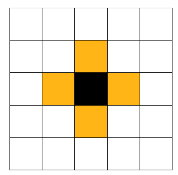
Agents in the Axelrod Model interact probabilistically with neighboring agents on the grid based on their degree of similarity. Here, a "neighbor" of a given agent is defined as any agent located one unit step away from the chosen agent (see Figure 1), and the similarity of two agents is based on the fraction of traits the two agents share.
At the start of the simulation each agent is assigned an initial set of random trait values. The cultural states of the agents are updated as follows: First an agent is selected at random along with one of its neighbors; this selection process is referred to as an “event.” The probability \(P_{i,j}\) that this selected pair (agent \(i\) and its neighbor, agent \(j\)) will then interact is computed from their degree of cultural overlap \(l_{i,j}\), defined as
| \[l_{i,j}=\sum_{f=1}^F\delta_{\sigma_i^f,\sigma_j^f} \] | \[(3)\] |
| \[P_{i,j}=\frac{l_{i,j}}{F}. \] | \[(4)\] |
Observe that this probabilistic rule implements the idea of homophily, wherein two neighboring agents are more likely to interact the more similar they are. Note that if two agents share no features (i.e., \(\sigma_i^f \neq \sigma_j^f \hspace{4mm} \forall f \in [1...,F]\)), then they have zero probability of interacting. When a pair of agents do interact, they will become more culturally similar, as follows: a random un-shared feature is selected and the chosen agent will change its trait value (for that feature) to that of its neighbor. This interaction rule implements the notion of cultural assimilation.
These simple dynamical rules lead to some interesting behaviors. Most notably, the twin influences of homophily and assimilation do not always lead to a purely homogeneous state (a mono-culture), but rather the agents can settle down into a final configuration characterized by several distinct cultural regions on the grid, wherein all agents within a given region are completely identical to one another, but share no common traits with agents in bordering regions. At this stage no further agent-agent interactions are possible and the system remains frozen in this final configuration known as an "absorbing state."
Axelrod’s simple model of cultural dissemination demonstrating that homophily and assimilation can yield heterogeneous societies has since been extended and generalized. For instance, the effect of a “mass media” agent was studied by Shibanai et al. (2001); see also Daley & Kendall (1964); Peres & Fontanari (2012); Rodríguez et al. (2009). The effect of noise, or “cultural drift" in the form of random perturbations of cultural features (Gandica et al. 2013; Klemm et al. 2003; Parisi et al. 2003), the interaction via complex networks rather than a grid (Pfau et al. 2013; Reia & Fontanari 2016), and the effect of increasing the neighborhood size (Stivala & Keeler 2016) have also been investigated. One interesting class of extensions of Axelrod’s original model which has received some attention to date, and which is the subject of this paper, involves incorporating the effects of social influence from all neighbors in an agent’s local neighborhood (i.e.,”social influence models"). In particular, in the classic Axelrod Model, during each interaction an agent will only directly compare itself to a single selected neighbor before potentially assimilating (so-called ‘one-to-one’ communication); in this case, the presence of the agent’s other equidistant neighbors has no immediate effect. In contrast, social influence models directly incorporate the effects of these other neighbors (i.e., ‘many-to-one’ communication) in an attempt to capture various aspects of local social dynamics.
Indeed, a variety of models exploring alternative communication schemes differing from that of Axelrod have been proposed (see, e.g., Parisi et al. 2003; Flache & Macy 2011). Seminal works on opinion dynamics/bounded confidence models by Hegselmann & Krause (2002) and Deffuant et al. (2000), for instance, take different approaches to many-to-one and one-to-one communication. Related issues are also addressed in social influence models described by Abelson (1964) and Friedkin & Johnsen (2011). And in more recent work by Keijzer (2018), a one-to-many communication scheme is explored in the context of online social networks, wherein a single online agent can potentially influence large numbers of other agents.
In what follows we first provide some general background on social influence models of cultural dissemination and introduce the main variant that is the focus of this paper (Section 2). In Section 3 we describe our main numerical findings and associated analysis. In Section 4 we introduce several new metrics for describing the nature of the absorbing state found in these models. These measures constitute potentially important new tools for the general study of agent-based cultural dissemination models, and their utility is not limited to the particular class of social influence models studied here.
Social Influence Model
Background
Kuperman (2006) has previously introduced several Axelrod-like models of cultural dissemination which incorporate a form of social influence factor (referred to by Kuperman as “cultural affinity”) similar in spirit to that which will be considered here. In one such model studied by Kuperman, during an interaction the selected agent will compare a randomly selected feature with that of its chosen neighbor, but rather than automatically changing its trait value for that feature to match that of its neighbor it will first survey its entire local neighborhood and will only change its trait value if doing so would increase the total number of matches the agent has with its neighbors on the given feature. If changing the trait value would result in fewer total matches with neighbors, no switch is done. In cases of a tie the agent would change its trait value with probability 0.5. As will be described shortly, our model of social influence is similar but avoids a hard cut-off in the trait-switching rule by employing instead a probabilistic trait-switching rule which allows for more malleability in its representation of everyday social interactions. Kuperman (2006) also introduced a second social influence-type model in which an agent does the same evaluation as in the first, but rather than just examining the neighbors for the selected feature, the agent looks at the overall overlap for all features in determining whether to switch the trait for the selected feature. Again, this model utilizes a hard cut-off, majority rule for trait assimilation rather than the more fluid, probabilistic trait-switching rule that we will consider. We do note, however, that one (analytical) advantage of Kuperman’s hard cut-off rule is that it allows for the introduction of a Lyapunov function to determine local stability at a given time step, without having to wait for the numerical model to reach a final absorbing state as Axelrod did.
Flache & Macy (2011) also analyzed a cultural dissemination model involving social influence. In this model, an agent is randomly selected and then will interact with some to all of its neighbors based on homophily, wherein the agent decides whether or not to interact based on the proportion of all features that are shared by the agent and its neighbor. (In this model, there is also probability \(r'\) that the decision to interact will be reversed.) After the agent chooses the neighbors to interact with, these neighbors are gathered in an influential set \(S\) and the agent chooses randomly one of its features which is different from at least one of the neighbors in the set \(S\). The agent will then adopt a new trait value so that after adoption, the new trait is dominant in set \(S\). However, if there is more than one trait that satisfies the above rule, the agent will randomly select one from among these traits. Flache & Macy (2011) find that this form of social influence helps to maintain a diversity of cultures and in fact produces more culturally distinct regions as the grid size is increased, in contrast to Axelrod’s original model where increasing grid size decreases cultural diversity and leads to a more mono-cultural state.
A probabilistic social influence model
The analysis of social influence studied in this work differs from the influential earlier works of Kuperman (2006) and Flache & Macy (2011) in two important respects. First, the interaction rules considered in our model have an intrinsic probabilistic component (based on a certain weighting of the agent’s local neighborhood) that renders agent-interaction outcomes less rigid compared to prior models employing deterministic rules with hard cutoffs and fixed outcomes. Secondly, unlike those previous works, our analysis is highly focused on quantifying the degree of cultural heterogeneity in a social influence network once it settles into an absorbing state, and thus should be viewed as complementary to those other works. Importantly, we introduce a number of new metrics for assessing the heterogeneity and related geometric aspects of the absorbing states which have broad applicability. Our model also retains the original simplicity of Axelrod Model in that during any interaction an agent will still only be able to switch its trait value for a specific feature to that of its selected neighbor, unlike the more complicated scenario examined by Flache & Macy (2011) which considers a “modal” trait from a group of neighbors and also incorporates the possibility of reversing an interaction. This simplicity yields some new insights into the effects of social influence in such models, including the underlying dynamical mechanisms responsible for the system’s behaviors.
We construct our Social Influence Model by introducing one extra step into the dynamical update rules used in the original Axelrod Model. Just as before, we start by assuming a randomly selected agent \(i\) and one of its neighbors (agent \(j\)) will interact with probability given by Equation 4, thereby incorporating homophily into the model. Assuming the pair do interact, a random unshared feature \(f\) is then selected (i.e., a feature for which the two agents have different associated trait values). The new social influence component now comes into play as follows: Rather than agent \(i\) automatically switching its trait value to match that of its selected neighbor (i.e., \(\sigma_i^f \rightarrow \sigma_j^f\)) as in the original Axelrod Model, instead agent \(i\) first surveys its local neighborhood to probabilistically assess how favorable such a switch would be. In particular, the agent will be less inclined to switch its trait to that of the selected neighbor agent \(j\) if doing so would lower agent \(i\)’s overall concordance on that trait with all of its other neighbors. More precisely, let \(N_i\) denote the local neighborhood of agent \(i\), which is defined here to include agent \(i\)’s four nearest neighbors (see Figure 1) plus agent \(i\) itself. Agent \(i\) surveys its neighborhood and counts the total number of its neighbors that share its trait value \(\sigma_i^f\). We refer to this number as the occurrence \(O_i(\sigma_i^f)\) of trait \(\sigma_i^f\), defined as:
| \[O_i(\sigma_i^f) = \sum_{n \in N_i}\delta_{\sigma_n^f,\hspace{1mm}\sigma_i^f}, \] | \[(5)\] |
| \[O_i(\sigma_j^f) = \sum_{n \in N_i}\delta_{\sigma_n^f,\hspace{1mm}\sigma_j^f}. \] | \[(6)\] |
| \[Q^{f}_{i,j}=\frac{O_i(\sigma_j^f)}{O_i(\sigma_i^f)+O_i(\sigma_j^f)}. \] | \[(7)\] |
To further clarify the effects of social influence, we highlight here some aspects of the switching probability described by Equation 7. As a reminder, we reiterate that in the local trait occurrence counts (Equations 5 and 6) defined above, the summations are over agent \(i\)’s entire neighborhood \(N_i\), which by definition includes not only agent \(i\)’s four nearest neighbors but also agent \(i\) itself. So, for example, in the extreme case where agent \(i\) and all of its neighbors except agent \(j\) share the same trait for the given feature \(f\), then the switching probability is relatively low, namely \(\frac{1}{5}\) (i.e., agent \(i\) is unlikely to change its trait since it is already in harmony with most agents in its local neighborhood). On the opposite extreme, consider an agent who is entirely surrounded by neighbors whom all share a common trait value which differs from that of agent \(i\) itself. In this case, the agent is in the minority and the switching probability becomes quite large, namely \(\frac{4}{5}\), indicating that the agent has a high chance of assimilating. Note here, however, that the model allows for some degree of “stubbornness,” or perhaps “free will,” since an outlier agent can still potentially retain its minority trait despite the homogeneity of its local neighbors.
To summarize, in our Social Influence Model there is an event (i.e., the random selection of an agent \(i\) and one of its neighbors \(j\)), an interaction probability \(P_{i,j}\) (determining if selected agents \(i\) and \(j\) will interact), and, when an interaction does occur, a switching probability \(Q_{i,j}^f\) (determining if agent \(i\) will switch its trait value for feature \(f\) to that of agent \(j\)). The switching probability incorporates the social influence of other agents in the given agent’s local neighborhood.
Results and Discussions
In this section, we present our major observations and discuss the implications of the added social influence factor compared to the original Axelrod Model. Our focus is on the level of cultural heterogeneity/homogeneity produced once the system settles into a final absorbing state. This yields not only a better understanding of the role of social influence in cultural dissemination, but also provides some deeper insights into Axelrod’s original model.
For the ensuing discussion of heterogeneity/homogeneity, we first introduce some basic terminology.1 As the agents on the lattice interact and evolve, distinct cultural regions can develop. Here, a “cultural region” denotes a group of adjacent, culturally identical agents which share all the same traits as one another at some moment in time. Cultural regions are generally somewhat fluid – they can morph and even dissolve owing to ongoing interactions between the agents just inside the cultural region and the neighboring agents just outside the region. A slightly stronger concept is that of a “cultural zone,” which is a cultural region of identical agents with the added property that the agents inside the zone have no traits in common whatsoever with agents that lie just outside the zone’s border. This means that no direct interactions can occur between the agents just inside and just outside the zone boundary since they share no common traits (see Equation 4). Hence cultural zones tend to be more stable structures than cultural regions. Note, however, that this does not mean that once a zone forms it will remain intact throughout all time. Indeed, cultural zones can themselves evolve and even dissolve. This is because outside agents which are not part of a cultural zone are continuing to update and change their trait values, and eventually some of the agents which lie just outside the zone boundary (and which formerly had no traits in common with the agents inside the zone) now might share some common traits with them – in other words, the cultural zone has now gone back to being a cultural region in which the agents on either side of the region’s border can interact and evolve owing to the presence of these common shared traits. Finally, we note that once the entire system eventually settles down into its fixed, final configuration (the “absorbing state”), all further spatiotemporal evolution ceases and the system essentially “freezes” into a set of distinct, static, cultural zones. We refer to these as “frozen zones.” This is the asymptotic behavior that we will primarily focus on; however, as we will show, to understand this asymptotic behavior it is necessary to also understand the dynamical processes (i.e., the formation, dissolution, and evolution of cultural regions and zones) leading up to the absorbing state.
Amplification of heterogeneity
Our first finding, illustrated in Table 1, concerns the number of distinct zones in the absorbing states. Data derived from 100 runs of both the Social Influence Model and the Axelrod Model on a \(30\times30\) grid, with five features (\(F=5\)) and ten traits per feature (\(Q=10\)), shows that the Social Influence Model has many more frozen zones compared to the corresponding Axelrod Model at those same parameter values.
| Social Influence Model | Axelrod Model | |
|---|---|---|
| Average number of frozen zones | 8.0 \(\pm\) 0.3 | 1.34 \(\pm\) 0.06 |
| Average number of events | 23,534,000 | 7,413,000 |
| Average number of interactions | 376,200 | 1,821,000 |
The numerically observed amplification of heterogeneity (i.e., increase in the number of frozen zones) under social influence compared to the Axelrod Model holds for a broad spectrum of different parameter choices \((F,Q)\), as illustrated in Table 2. As is seen, direct comparison of the two models at the same parameter values shows that the inclusion of the social influence factor increases heterogeneity compared to the Axelrod Model. We seek to elucidate the dynamical mechanisms underlying this effect.
| # of Frozen Zones | |||
| Social Influence | Axelrod | ||
| (F,Q) = | (5,5) | 1.1 | 1 |
| (5,10) | 8 | 1.34 | |
| (5,15) | 59 | 10 | |
| (10,5) | 1 | 1 | |
| (10,10) | 1.12 | 1 | |
| (10,15) | 2.1 | 1.04 | |
In broad intuitive terms, the increase in overall heterogeneity might seemingly arise in part because, under the action of social influence, the borders of a cultural region tend to be less susceptible to infiltration by outside, neighboring agents. Consider, for instance, an agent just inside the border of a cultural region, and focus on some particular feature \(f\) with trait value \(q\). This agent shares this same trait value with all its neighboring agents inside its cultural region. Thus, when that agent interacts with a neighbor with a different trait value \(q'\) residing just outside the cultural region, under the Social Influence Model the agent has only a low probability of switching its trait value \(Q_{i,j}^f << 1\) compared to Axelrod-like models where, in effect, \(Q_{i,j}^f = 1\). Thus, without social influence, boundaries between cultural regions tend to be more vulnerable to the introduction of new traits, and the resulting dissolution of borders increases the likelihood that the final absorbing state will be relatively homogeneous, or perhaps even mono-cultural. However, this simplistic description is insufficient. The actual dynamical portrait is more nuanced, and it is necessary to examine more deeply the underlying mechanisms and processes by which distinct cultural regions and zones can form and evolve. In what follows we isolate and adjust various parameters of the models to better understand these mechanisms responsible for the increase in heterogeneity. Our work enjoys certain parallels with the important earlier findings of Flache & Macy (2011) on the effects of social influence. Although the Social Influence Model studied here (and our focus on the properties of the absorbing state) differs from that of Flache & Macy (2011) in multiple respects (e.g., the latter incorporates selection error, “modal” traits, cultural perturbations, and a different social interaction scheme), nonetheless we will observe a qualitative harmony between the two models, which speaks to the robustness of the underlying mechanisms responsible for the amplification of heterogeneity under social influence.
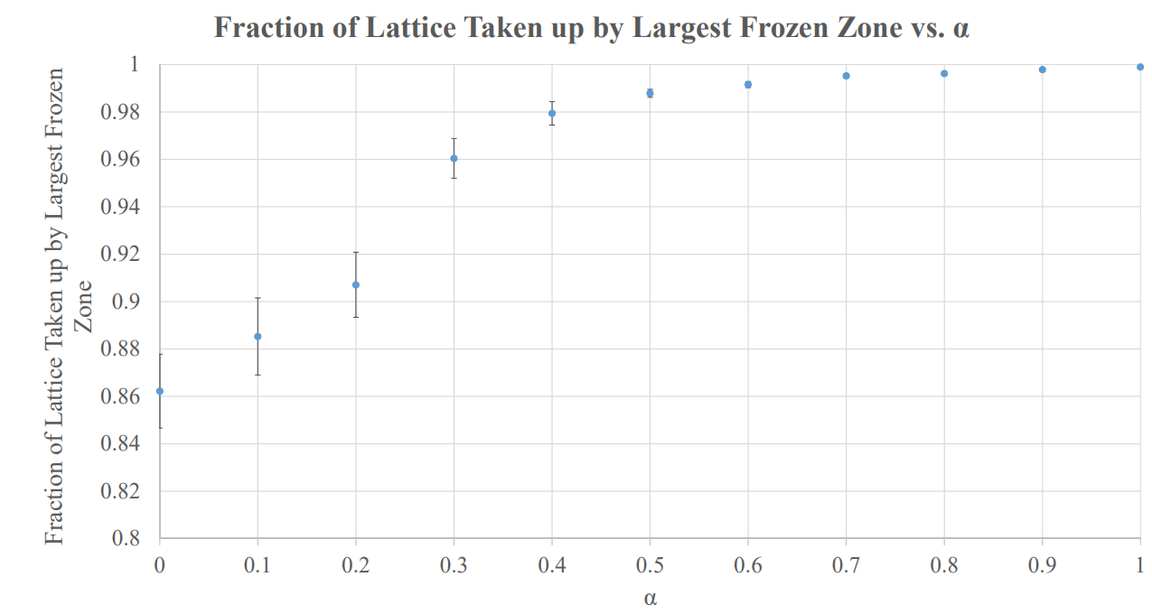
Before proceeding, we remark that some additional preliminary insight into the amplification of heterogeneity under social influence can be obtained by performing a type of sensitivity analysis, wherein one smoothly transitions between the Social Influence Model and the original Axelrod Model. Recall that the key difference between the two models is that in the former there is a socially derived switching probability \(Q_{i,j}^f\) (see Equation 7) that is determined by how well a given agent “fits” with its local neighbors, whereas in the Axelrod model the effective switching probability is essentially unity. By introducing an auxiliary parameter \(\alpha\) which varies between 0 and 1, we can define a modified switching probability \(W_{i,j}^f\) via:
| \[W^{f}_{i,j}=(1-\alpha)Q^f_{i,j}+\alpha.\] | \[(8)\] |
In what follows we conduct a detailed examination of various facets of the Social Influence Model to better understand the effects of social influence on cultural assimilation, and identify and analyze the underlying dynamical mechanisms responsible for the behaviors seen.
Heterogeneity and lattice size
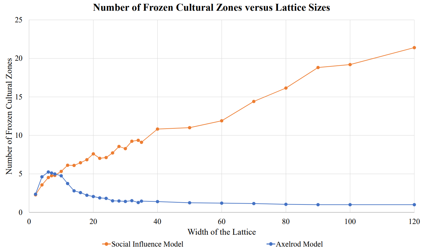
One intriguing and relevant observation from the original Axelrod Model is its behavior over varying grid sizes. As one can see in Figure 3, as grid size increases, the average number of frozen cultural zones in the Axelrod Model initially increases, but as the grid size surpasses \(6\times6\) the number of frozen zones begins to decrease and eventually a mono-cultural state reigns, in which the majority of trials result in an absorbing state that is completely homogeneous. In contrast, in the Social Influence Model – at those same parameter values \(F,Q\) – the number of frozen zones continues to increase (somewhat linearly) with grid size. This qualitative distinction between the observed behaviors of the two models is surprising because the underlying differences in the agent-agent interaction rules between the Axelrod Model and the Social Influence Model may appear to be relatively modest. Recall that the only modification made by the Social Influence Model is the inclusion of a simple switching probability \(Q_{i,j}^f <1\) which takes into account an agent’s cultural affinity with its local neighbors, unlike the Axelrod Model. An analysis (below) of the underlying processes governing the formation and growth of distinct cultural zones will help to clarify the distinctions that emerge in the behaviors of the two models under the same parameter values \(F,Q\), and ultimately help elucidate the mechanisms responsible for the amplification of heterogeneity under social influence. We note that the behavior displayed in Figure 3 also occurs at other parameter values \((F,Q)\); see, for instance, Figure 21 in Appendix F which is taken at \((F,Q)=(7,15).\) Moreover, as an additional point of comparison, we also constructed a different social influence model (in Appendix E) - a stripped down version of an earlier social influence model by Flache & Macy (2011) - and observe a similar increase in heterogeneity with lattice size, which suggests certain universal dynamical effects are at play.
Before delving into these causes, we briefly remark here that, from the interesting work of Castellano et al. (2000, 2009)(see also Klemm et al. 2003), we know that in the original Axelrod Model the choice of simulation parameter \(F=5\) lies on the “order” side of a non-equilibrium, order-disorder phase transition, in contrast to what we observe (for the same parameter choice) in our Social Influence Model. While the issue of the existence and nature of phase transitions in such models is quite interesting and discussed further in Appendix C, it remains somewhat outside the central focus of this paper. Instead, for purposes of understanding amplification of heterogeneity under social influence compared to the Axelrod Model (as seen in Table 2 and Figure 3), we concentrate on a detailed examination of the dynamical processes underlying zone formation in these models.
In his original paper, Axelrod lays out two general mechanisms that govern the system’s behaviors at different grid sizes, and we will analyze these mechanisms in both the Axelrod Model and Social Influence Model. The first mechanism, which we will refer to as a “multiplicity effect,” is fairly straightforward. The multiplicity effect reflects the observation that the number of possible frozen cultural zones increases with grid size owing to the presence of more agents (i.e., borrowing language from statistical mechanics, more microstates are possible with larger lattices). This explains the initial growth seen in Figure 3 in the number of frozen zones for the Axelrod Model. But there is a second competing effect at play in the Axelrod Model which tends to favor homogeneity at large lattice sizes. This second mechanism, which we will call “the dominant-regions effect” is more complicated. Generally, this effect states that, given two similar regions that can interact, during their subsequent dynamical evolution the larger region is more likely to completely eliminate the smaller region than vice versa, leaving just a single cultural region. As Axelrod (1997) explains, this process can be understood as follows: Imagine a simplified model with 10 agents in total, lined up along a one-dimensional lattice. Suppose these agents have two cultural features, each with two possible trait values, 0 and 1. Next imagine that, at the start of the simulation, the grid is divided into two cultural regions, where all agents on the left half of the grid are in cultural state \([0,0]\) while those on the right half are in state \([0,1]\), as shown: \(\textbf{[0,0] [0,0] [0,0] [0,0] [0,0] [0,1] [0,1] [0,1] [0,1] [0,1]}\). Any change to the current configuration of the system will be initiated by the two center agents on the boundary separating the two cultural regions. These two agents have an equal probability of being selected and having their cultural vector changed to that of the other agent, leaving two possible outcomes, namely
| \[\begin{aligned} \textbf{[0,0] [0,0] [0,0] [0,0] [0,0] [0,0] [0,1] [0,1] [0,1] [0,1] }\end{aligned}\] | \[(9)\] |
| \[\begin{aligned} \textbf{[0,0] [0,0] [0,0] [0,0] [0,1] [0,1] [0,1] [0,1] [0,1] [0,1] }\end{aligned}\] | \[(10)\] |
Depending on the agent selected, one cultural region will grow and the other will shrink. The system will continue to evolve in this manner until one region completely absorbs the other and no further interaction is possible. Since only one pair of agents can interact at a time, and since they have an equal probability of being changed, the entire scenario can be effectively modeled as a random walk. In the scenario described above, both regions initially started with five agents, and thus either region is equally likely to absorb the other. However, if the initial sizes of the cultural regions were different, then the probability of the larger region absorbing the smaller one would be higher because the larger region would have a shorter random walk. This means that the probability of a region absorbing another region varies directly with size. Although the above illustration of the dominant-regions effect was for a very simple one-dimensional version of the Axelrod model, the same basic premise could presumably hold for more complex, higher-dimensional models.
As a test of this idea, we conducted 1,000 trials of both the Axelrod Model and the Social Influence Model on the (2-dimensional) lattice of agent states shown in Figure 4.
Note that this starting lattice (on the left of the figure) has one large dominant cultural region and five smaller regions that each share only one trait with the dominant region. The simulations reveal that once the system reached a final absorbing configuration, the result was a mono-culture in a large majority of the runs. Specifically, the simulations resulted in a mono-culture in 75\(\%\) of the runs for the Axelrod Model and in 90\(\%\) of the runs for the Social Influence Model. This indicates that the dominant-regions effect is at work in both models (and appears in fact to be modestly stronger in the Social Influence Model). This effect helps to explain the decline in the overall level of heterogeneity seen in the Axelrod model, since larger grids facilitate larger cultural regions, and by the dominant-regions effect these larger regions will absorb the smaller regions around them, becoming even more dominant as they grow, thereby creating a positive feedback loop that typically results in a final, mono-cultural absorbing state. In short, for the Axelrod model we see that the multiplicity effect favoring heterogeneity wins out over the dominant-regions effect for small lattice sizes, but for large lattice sizes the dominant-region effects favoring homogeneity begins to predominate (Figure 3). However, this explanation seems to fail for the Social Influence Model and in fact presents a paradox: Given that the dominant-regions effect is in fact moderately stronger in the Social Influence Model than the Axelrod model, why does the number of frozen zones in the Social Influence Model continue to increase with region size (Figure 3)?
To resolve this seeming paradox, we must examine more closely the cultural profile of the final mono-culture and the underlying processes that led to it. The first key observation is that the cultural profile of the mono-culture in the final absorbing state is not necessarily the same as the cultural profile of the initial dominant region. As a dominant region absorbs the surrounding regions, it can sometimes adapt, taking traits from the smaller regions before subsuming them. This occurred more frequently in the Axelrod Model than the Social Influence Model (e.g., data associated with Figure 4 reveals that when a mono-culture formed, the final absorbing state differed from the initial dominant region in about 63% of trials for the Axelrod Model but only in about 9% of trials for the Social Influence Model). The reduced probability of trait exchange in the Social Influence Model (owing to \(Q^f_{i,j} < 1\)) significantly increased the overall resistance of large cultural regions from changing as a whole. This aspect of the Social Influence Model provides a clue in explaining its behavior, as we now describe.
To start, recall that a cultural region is a group of adjacent, culturally identical agents bordered by agents possessing a somewhat different (but still overlapping) trait profile, whereas a cultural zone is a special case of a cultural region in which the agents immediately outside the region’s border have no traits in common with the agents inside the region. Accordingly, the agents inside a zone cannot directly interact with agents just outside the border. Hence zone borders, though they can change over time, tend to be more structurally stable than regional borders. And it remains true that, by the dominant-regions effect, large zones, if they remain intact, tend to absorb smaller regions over time.
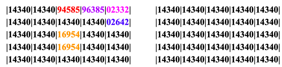
Now consider the initial cultural matrix shown on the left in Figure 5. It is composed of a dominant region (in black), two smaller regions (orange and green), and a zone (in red).
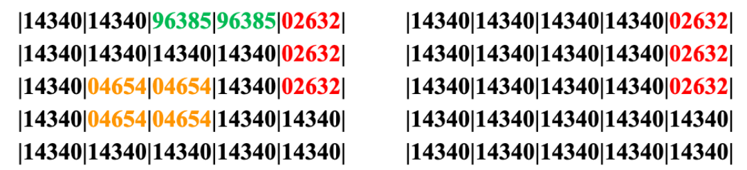
Focus on the behavior of the red zone. Although agents in the red zone are initially completely dissimilar to the agents that border them and hence cannot directly interact with them, it is still possible for the red zone to change over time and potentially be absorbed by the dominant region. To see how this can come about, note that while the red region has no traits in common with the bordering black and green regions, it does share two traits in common with the faraway orange region. And note moreover that the orange and green regions each have a trait in common with the black region and hence can exchange traits with it. Therefore, it is possible for an orange-region trait (for example, the middle “6” in [04654]) to partially infiltrate into the black region and subsequently begin interacting with agents in the red zone, which previously was not possible. Likewise, trait propagation is also possible via orange \(\rightarrow\) black \(\rightarrow\) green \(\rightarrow\) red. In this manner the initial red zone need not always remain intact and in fact could ultimately be absorbed. In 10,000 simulations of the Axelrod model (with initial cultural matrix shown in Figure 5, left), the model produced a mono-culture in 68\(\%\) of the runs; 19\(\%\) of runs resulted in the dominant (black) region maintaining its original profile, meaning that it did not pick up any traits from the orange [04654] region or green [96385] region when they were assimilated. The original red zone ultimately disappeared via interactions with outside agents in about 70\(\%\) of the Axelrod runs (via the intermediary action of the black agents assimilating the traits from the orange region, i.e., through the middle “6”). In contrast, in the Social Interaction Model, the red zone proved much more robust, and a mono-culture was produced in only 38\(\%\) of the runs. In 59\(\%\) of the runs the dominant (black) region maintained its original cultural profile (i.e., did not assimilate traits from the orange region it consumed). The red zone remained unchanged in 62\(\%\) of the runs, which also suggests a lack of trait assimilation.
These observations help explain why the Axelrod model results in declining numbers of frozen zones with increasing grid size, while in the Social Influence Model the number of zones steadily increases (Figure 3). In both models both the multiplicity effect (favoring heterogeneity as lattice size is increased) and the dominant-regions effect (favoring homogeneity as larger cultural regions absorb smaller cultural regions) are at work. And indeed the the dominant-regions effect is actually more pronounced in the Social Influence Model. However, in the Social Influence Model agents within neighboring regions are far less able to spread around cultural traits in order to break zones (even though larger regions still have a tendency to absorb smaller regions). This resistance results in stronger zones, which, in combination with the multiplicity effect, ultimately leads to an overall increase in the number of frozen zones with lattice size in the Social Influence Model. Further elaboration and additional related data is provided in the next two subsections. That said, despite this evidence we caution that it would be premature to definitively conclude that this trend (Figure 3) is truly asymptotic, since for sufficiently large lattice sizes (beyond those numerically explored here), the curve for the Social Influence Model could ultimately turn back down owing to unanticipated nonlinear effects.
Zone size distribution
We next examine the distribution of the sizes of frozen cultural zones. Figure 6 shows the results a \(30\times30\) grid with \(F=5\) and \(Q=10\) averaged over 100 runs. In both the Axelrod Model and the Social Influence Model, the majority of frozen zones were either very small - i.e., consisting of just one or two agents - or very large, covering most of the lattice. But there were some important differences. The Social influence model, for instance, exhibited on average 3.8 single-agent zones per run, compared to just 0.2 single-agent zones for the Axelrod Model. This can be understood as follows. Due to the exceedingly large number of possible feature/trait combinations for an agent (\(F^Q\)), during the initial random setup of the individual agents’ cultural profiles, the probability that a given agent will have no traits in common with any of its nearest neighbors (and hence constitute a single-agent zone) is \((1-1/Q)^4 \approx 0.66\). As described above, zone boundaries tend to be more robust in the Social Influence Model and less likely to be subsumed by large surrounding regions, so we would expect more single-agent zones to have survived once the system settles into an absorbing state compared to the Axelrod Model.
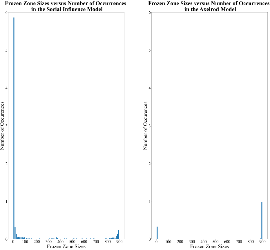
In addition, observe from Figure 6 that the Social Influence Model had much greater variety in terms of sizes of frozen zones. For this model, small zones of size 1 and 2 were common, with about 3.8 occurrences per run and 0.9 occurrences per run respectively, along with a single large zone of size in the high 800’s. Notably, there were no zones of size 900 in any of the 100 runs of the Social Influence Model, i.e., no mono-cultures. A moderate sprinkling of intermediate size zones is also seen. In contrast, in the Axelrod Model, mono-cultures appeared in about 74% of runs, and intermediate-size zones containing between 13-885 agents were altogether absent. As discussed previously, in the Axelrod Model, the dominant-regions effect results in larger regions tending to consume smaller regions. As a result, almost none of intermediate-size regions survive once the system settles. On the other hand, the more resilient borders between cultural regions and zones in the Social Influence Model makes it more likely that smaller and intermediate sized regions will survive even in the presence of the dominant-regions effect, resulting in a modest number intermediate-size zones in the absorbing state. We point out that while our numerical data and analysis demonstrate that incorporating a social influence component into the Axelrod Model does, rather intriguingly, produce greater cultural diversity, nonetheless we also note that this diversity does not overwhelm and/or completely fragment the system in the parameter regimes we are studying. For instance, while the Social Influence curve in Figure 3 may superficially give the appearance of runaway growth in cultural diversity, this is not the case. Indeed, one sees from the data that for a \(30\times30\) lattice with 900 agents, there are only about 8 distinct zones, and for a lattice with 14,400 agents there are only about 22 zones, and moreover, in these cases there is typically just one very large cultural zone and the rest tend to be relatively small. Likewise, Figure 6, while clearly illustrating the notable increase in diversity arising from social influence, also shows that the number of single-agent zones remains rather modest (i.e., about 4 culturally isolated single-agent zones out of 900 agents). These observations are also reflected in the data in Figure 2.
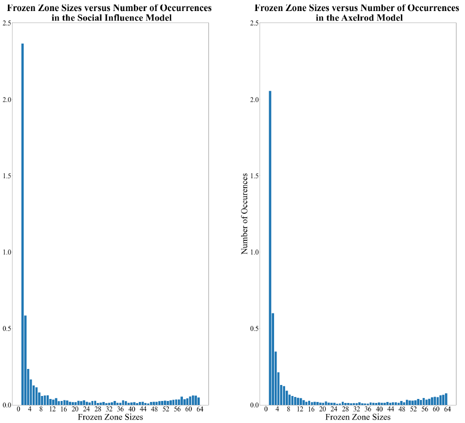
It is also interesting to briefly consider frozen-zone size distributions using a small \(8\times8\) lattice, which, as seen in Figure 3, corresponds to the lattice size at which the average number of frozen zones in both the Social Influence Model and Axelrod Model are nearly equal. The zone size distributions are shown in Figure 7. Notably, we find that these distributions are highly similar, suggesting that the differences in the dominant-region effects in the two models first become manifest for grid sizes larger than \(8\times8\).
Lastly, we briefly comment here on the effects of neighborhood size on the heterogeneity of the absorbing state. All of the preceding simulations were done assuming each agent (in the interior of the lattice) has 4 nearest neighbors, i.e., that lie one unit away in the taxicab metric. One could instead imagine enlarging the neighborhood size to 12, corresponding to neighbors which are two units away or less in the taxicab metric. As we might anticipate based on prior work on the Axelrod Model, in the Social Influence Model we observe that increasing the neighborhood size tends to decrease the average number of frozen zones. We also observe that while the number of frozen zones decreases, the sizes of the smaller frozen zones tends to increase. Details on the effects of increasing neighborhood size are described in Appendix D; see in particular Figures 18 and 19.
Approach to the absorbing state
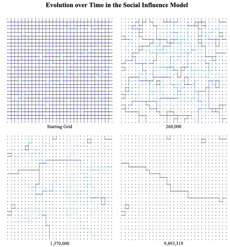
We next examine the dynamical progression of the system during its journey towards the final absorbing state. Referencing Table 1, we first note that the Social Influence Model requires almost three times as many events to reach an absorbing state, but with approximately five times fewer total interactions. For instance, for the chosen simulation parameters, it takes the Social Influence about 23.5 million events and nearly 380,000 interactions to reach an absorbing state while the Axelrod Model requires 7.4 million events and 1.8 million interactions. These trends can be understood as follows: Recall that in the Axelrod Model the agents’ cultural profiles can change more easily, and thus cultural regions and zones tend to be relatively fluid. Accordingly, the number of interactions required for the system to finally settle into an absorbing state will be higher than in the corresponding Social Interaction Model where agents and cultural boundaries tend to be more rigid. On the other hand, each interaction in the Social Interaction Model will require more attempts (i.e., events) before it actually occurs, since the probability that an event produces an interaction is lower (since \(Q_{i,j}^f < 1\)) than in the Axelrod Model, resulting in a larger number of events for the Social Interaction Model. But we can garner a deeper understanding of the system’s behavior by examining the evolving cultural states as they progress towards the final absorbing state. By recording the cultural profile of the system at different stages of its evolution2, one can visualize how agents form, destroy, and re-form borders over a period of time as illustrated in Figures 8 and 9. The Social Influence Model (Figure 8) tends to result in more isolated one-agent and two-agent zones that form early on in the simulation and which remain isolated and intact all the way through to the absorbing state. For instance, the two-agent zone in the upper-right corner of Figures 8 that appears sometime within the first 260,000 events is able to survive, unchanged, for the nearly 10 million events that follow. Meanwhile, in the Axelrod Model (Figure 9) one commonly sees dissolution of small zones (e.g., consider the two single-agent zones in the upper-left corner at 340,000 events), as well as the dominant-regions effect in which larger cultural regions tend to absorb smaller ones.
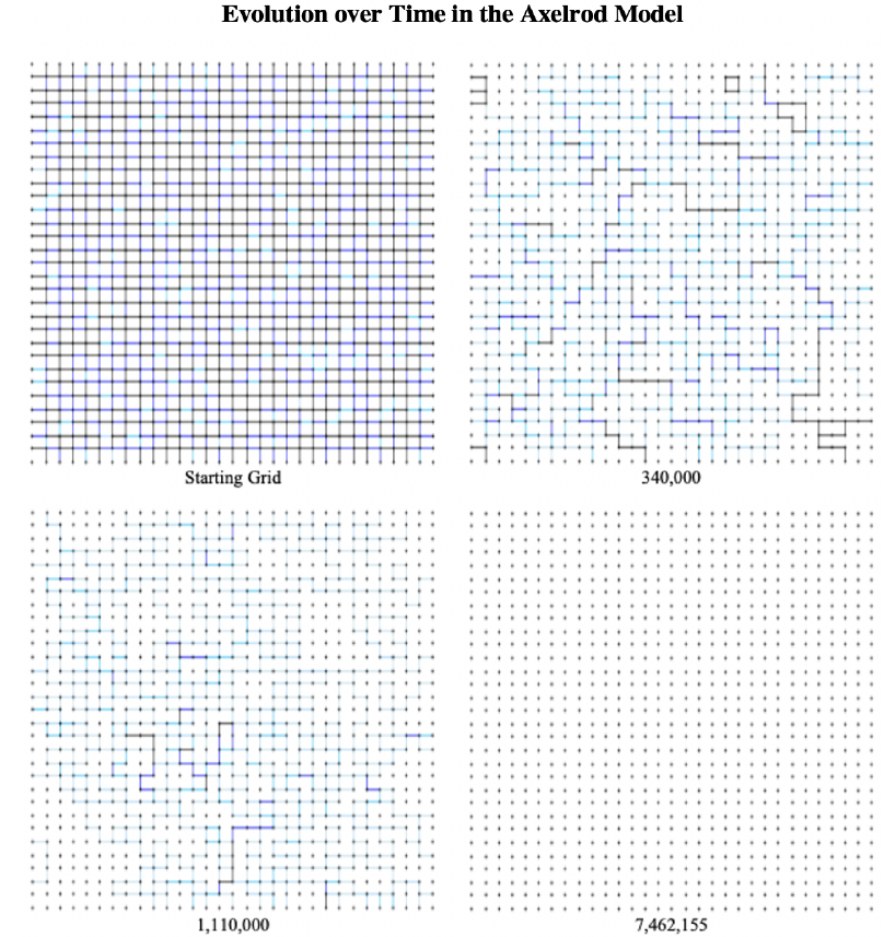
We next track the number of cultural states in each model over the course of their evolution to a final absorbing state. Figure 10 shows representative examples of these evolutions. Observe that the number of cultural regions in the Social Influence and Axelrod Model both initially decline sharply. However, the decline in Social Influence Model tends to be steep (e.g., it declines to 200 cultural regions after approximately 300,000 events whereas the Axelrod Model requires over 3,000,000 events to attain this same diminution) and then curve notably flattens for a long period. In contrast, in the Axelrod Model, after the initial rapid descent, the decline continues in a more moderate, relatively steady manner.
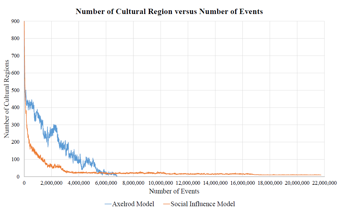
As can be seen in Figures 8 and 9, regions of identical agents tend to rapidly form relatively early in both the Social Influence and Axelrod models. This is because, due to the random assignment of initial traits, in the very early stages of the simulation an agent is unlikely to be surrounded by a culturally similar neighbors, so the social influence factor does not play a big role and thus the two models behave similarly (namely, the number of cultural regions declines rapidly as smaller regions are quickly assimilated by larger regions due to the dominant-regions effect). However, in the Social Influence Model, after this rapid reduction in the number of regions and zones, the subsequent rate of change slows dramatically since the social-influence effect is now heightened in these remaining regions and zones as the agents harden against further change. Thus, after the rapid drop in cultural regions, we see a slow decline in the number of regions until the absorbing state is reached. In contrast, the Axelrod Model exhibits a steadier, more consistent decline in cultural regions because the absence of the social-influence factor helps the boundaries between cultural regions and zones remain malleable and less likely to freeze in place.
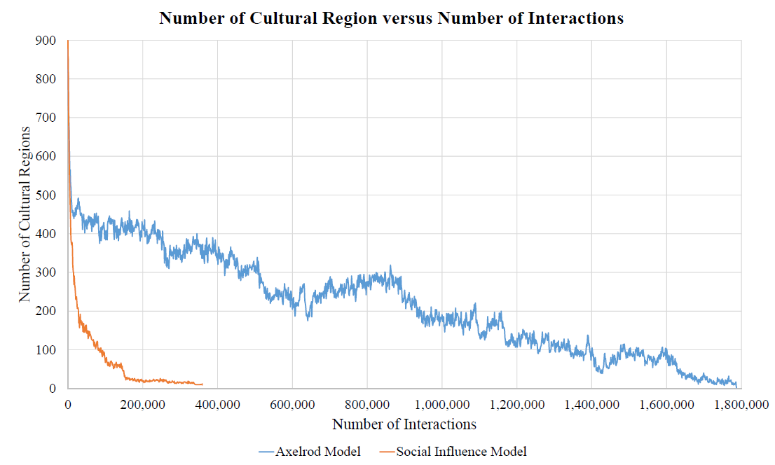
Lastly, we mention that as an alternative to looking at the model’s temporal evolution as a function of events (as in Figure 10), one could instead examine it as a function of events (see Figure 11). Both events and interactions can serve as reasonable proxies for "time," and thus Figures 10 and 11 are qualitatively similar. The quantitative difference in horizontal timescales in the two graphs is consistent with the numerical results of Table 1.
Cultural Heterogeneity Metrics
We next wish to quantitatively characterize the nature of the heterogeneity in the system, both during the course of its dynamical evolution and after it settles into a final absorbing state. In most previous works, as in Axelrod’s original analysis, heterogeneity has been primarily characterized by simply counting up the total number of distinct cultural regions and/or zones. While this serves as a very useful, basic tool, it throws away a great deal of potentially important information about the regions and zones. For example, a lattice with three zones could have two very small zones and one very large zone that subsumes nearly the entirety of the lattice, or instead the lattice might have three zones all of approximately equal size. Simply counting the total number of zones will not distinguish between these different scenarios. Likewise, a simple count of zones provides no information about the overall geometrical qualities of the frozen zones making up the heterogeneous absorbing state, and in particular does not differentiate between heterogeneous states made primarily of geometrically compact (e.g., square-shaped) frozen zones versus heterogeneous states whose frozen zones are highly filamentary in shape and/or have very course boundaries. Such considerations motivate our desire to construct novel metrics to quantify different aspects of heterogeneity in cultural dissemination models. We developed the following three measures, each capturing a unique facet of the system’s heterogeneity (aka ‘disorder’).
- Heterogeneity Metric 1 describes the relative dissimilarity of each agent on the grid to its neighbors based on differences in trait values.
- Heterogeneity Metric 2 is an entropic-based measure taking into account both the number of regions and their sizes.
- Heterogeneity Metric 3 measures the degree to which the frozen zones of a heterogeneous absorbing state are geometrically elongated in shape and/or have very rough boundaries (versus being compact and smooth).
Heterogeneity metric 1
Inspired by direct comparison in adjacent agents’ profiles, Vazquez et al. (2010) developed a metric for disorder in a binary system, where each agent either spoke language X or language Y or both X and Y:
| \[\rho = \frac{1}{2N_l}\sum_{\langle i,j \rangle}\frac{1-S_iS_j}{2} \] | \[(11)\] |
| \[\rho_1=\frac{1}{4 N(N-1)}\sum_{i=1}^{N^2}\sum_{j \in N_{i}^{'}}\left(1-\frac{l_{i,j}}{F}\right) \] | \[(12)\] |
The above metric \(\rho_1\), by design, compares each agent to each of its neighbors, and counts up the number of features that it does not share the same trait values with. This is repeated for all agents in the lattice. The result is then normalized, so that the resulting metric \(\rho_1\) is a number between 0 and 1 that quantifies the relative dissimilarity of each agent on the lattice to its neighbors, with 1 representing complete disorder (i.e., no agent shares any of the same trait values with any of its neighbors) and 0 representing complete order (i.e., every agent has the same trait value for each feature).
Heterogeneity metric 2
A second method of characterizing disorder is borrowed from statistical physics and is based on the idea of configurational entropy (see, e.g., Jaynes 1978). In the present context of cultural dissemination models, given the observed number and sizes of the cultural regions, we first estimate the number of possible geometrical rearrangements of these regions on the lattice. This number of rearrangements, called the multiplicity \(\Omega\), will be relatively small for lattices containing just a few, fairly large regions, and will be very high for lattices containing many small regions. We then define the entropy of the system to be \(\ln(\Omega)\), and use this as a new disorder metric for such systems.
Due to the complexity of calculating all possible lattice configurations for a given set of \(M\) regions of sizes \(S_i, i=1\ldots M\), several assumptions are used to simplify the computation of \(\Omega\). First, the regions are all assumed to be relatively square in shape,3 as seen in the upper and lower left images of Figure 12. This greatly simplifies the problem, as re-arranging squares on a lattice is much simpler than reorienting mismatched "Tetris" pieces (see, e.g., the upper right image of Figure 12).
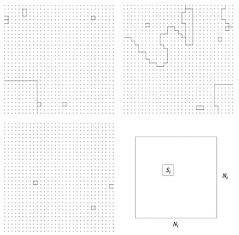
Second, to account for the space in the lattice being taken up by the regions of different sizes, we start with an empty lattice and imagine sequentially filling it, beginning with the smallest region and moving on to progressively larger regions. At each step in this iterative process, we look at the remaining space available in the lattice and treat this remaining space as though it were a smaller, square lattice, and then compute how many configurations are available to the current region as we insert it into this reduced lattice. We continue in this manner until the largest region has been inserted, at which point the full lattice is filled. The motivation for sequencing from small to large is based on the observation that small regions are effectively unconstrained in where they can appear within the lattice - e.g., a small region can easily appear as an island within a larger region. In other words, large regions are not effective at blocking small regions (see, for instance, the lower left graph of Figure 12).
Given these considerations, the metric itself is constructed as follows. Assuming that all regions of size \(S_i\) are squares with sides of length \(\sqrt{S_i}\) (where \(S_{i+1} \geq S_i\) for \(i=1...M\)), that the original lattice has size \(N^2\) with sides of length \(N\), and that \(N_i^2\) denotes the amount of lattice space remaining immediately prior to the insertion of region \(i\) (where \(N_1=N\)), then, as seen in the lower right image of Figure 12, region \(i\) can be positioned in \((N_i-\sqrt{S_i}+1)^2\) distinct ways. Note that as regions are sequentially inserted, the remaining space at each step is \((N_{i+1}^2=N^2-\sum_{j=1}^{j=i}S_j )\). Hence the total number of possible configurations for \(M\) regions of sizes \(S_i\) with \(i=1, \dots M\) under the given assumptions is:
| \[\Omega = \prod^M_{i=1}(N_i-\sqrt{S_i}+1)^2, \] | \[(13)\] |
| \[\ln(\Omega)= 2\sum^M_{i=1}(N_i-\sqrt{S_i}+1)\] | \[(14)\] |
| \[\rho_2 = \frac{2\sum\limits^M_{i=1}\ln(N_i-\sqrt{S_i}+1)}{\ln(N^2!)} \] | \[(15)\] |
We note that metric \(\rho_2\) is particularly sensitive to the number of small regions present in the system, since each of these can significantly increase the multiplicity \(\Omega\). This sensitivity is somewhat obscured by the natural logarithm that appears in the entropy, and further still by the normalization factor (since most absorbing states are nowhere near being maximally heterogeneous). Nonetheless, as a heterogeneity metric the relative size of \(\rho_2\) is strongly influenced by the number of small regions in the system.
Heterogeneity metric 3
While the previous two metrics \(\rho_1,\rho_2\) are useful for quantifying the average degree of dissimilarity between agents and the configurational entropy associated with the number and sizes of cultural regions on the lattice, neither provides direct information regarding the geometrical shapes of the different regions. For instance, regions or zones could potentially be elongated and filamentary in appearance with rough boundaries, or instead perhaps relatively compact with smooth boundaries. We thus introduce a new metric to characterize this geometric aspect of heterogeneity. The construction is fairly straightforward, and utilizes the fact that filamentary regions and/or regions with sufficiently coarse boundaries will tend to have a high fraction of agents on their border (relative to interior agents), whereas for compact regions with smooth boundaries this fraction will be much smaller. We define \(B_i\) to be the number of border agents for region \(i\); it is computed by summing up (over all agents in region \(i\)) the total number of external agents with whom an agent in region \(i\) shares a border. Note that in this counting process some external agents will be counted more than once if they happen to share borders with multiple agents in region \(i\). If region \(i\) with size \(S_i\) were perfectly square in shape with smooth boundaries and thus maximally compact, it would have \(4\sqrt{S_i}\) bordering agents. Thus the ratio \(B_i/4\sqrt{S_i}\) is a measure that reflects both the degree of elongation and the roughness of the boundaries of a region compared to a maximally compact region of the same size. We then average this ratio over all \(M\) regions in the lattice, and then subtract one from this average in order to measure the deviation of the regions’ geometry from perfectly smooth, compact squares. This yields the metric
| \[\rho_3=\left(\frac{1}{M}\sum_{i=1}^M\frac{B_i}{4\sqrt{S_i}}\right)-1, \] | \[(16)\] |
Lastly, we remark on some of the scaling properties of this geometrical heterogeneity metric. Consider a lattice of size \(N\times N\) containing \(M\) regions of various sizes and shapes. Now imagine simply enlarging the size of the lattice along with all the regions therein (while keeping the number and the shapes of the individual regions the same). Under this enlargement observe that \(\rho_3\) will remain unchanged, as expected, given that the overall shapes of the regions have been maintained. However, consider instead the case in which a particular region becomes progressively narrower (relatively speaking) as the lattice grows. For instance, consider a long rectangular strand of width one that runs the length of the lattice (i.e., size \(N\times1\)), and suppose that as \(N\) increases the width of this region remains one. Such a region thus becomes more and more filamentary in form as the lattice grows. In this case, the extreme geometry of this filament will dominate the metric \(\rho_3\), and it is easy to show that the metric will scale as \(\rho_3 \sim \sqrt{N}\). While we do not expect such filamentary strands which span the entire lattice to actually arise in models of the type considered here, nonetheless this argument shows that progressively roughening the boundary of a region will lead to a larger \(\rho_3\).
Disorder/heterogeneity analysis
We next use the above three heterogeneity metrics to gain deeper insights into the behaviors of the Social Influence and the Axelrod models, and in particular to better understand and quantify the emergence of heterogeneity.
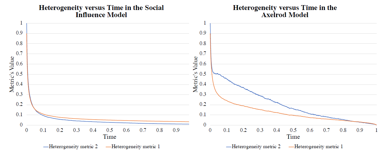
In Figure 13, we can see a clear distinction between the Social Influence and Axelrod models for the first two disorder metrics. In the Axelrod Model (right), both disorder metrics asymptote (at time=1) very close to zero, indicating the preponderance of a single ordered (homogeneous) absorbing state in a large fraction of the runs. The asymptotic values of \(\rho_1, \rho_2\) for the Social Influence Model are also very close to zero, though they do remain higher those for the Axelrod model (this small difference is somewhat obscured in the figure owing to the scale of the graph, and the normalization used for the metrics).
More interestingly, if instead we focus on the temporal evolution of these metrics rather than their asymptotic values, we see another revealing difference between the two models. Both models show a sharp initial drop in disorder followed by long plateaus, but observe that this drop-off is more rapid in the Social Influence Model. We can understand this finding as follows: In the Social Influence Model, owing to neighborhood interactions zones tend to form relatively quickly, and once formed tend to be dynamically robust, so that subsequent changes are slow and relatively minimal, which explains the long plateaus seen in the left image of Figure 13. In contrast, in the Axelrod model many more regions form initially which are more susceptible to subsequent changes compared to zones, and hence the temporal evolution continues for a longer period of time, resulting in a more gradual, steadier tapering off of disorder compared to the extended plateaus in the Social Influence Model. This effect is accentuated in the behavior of disorder metric \(\rho_2\).
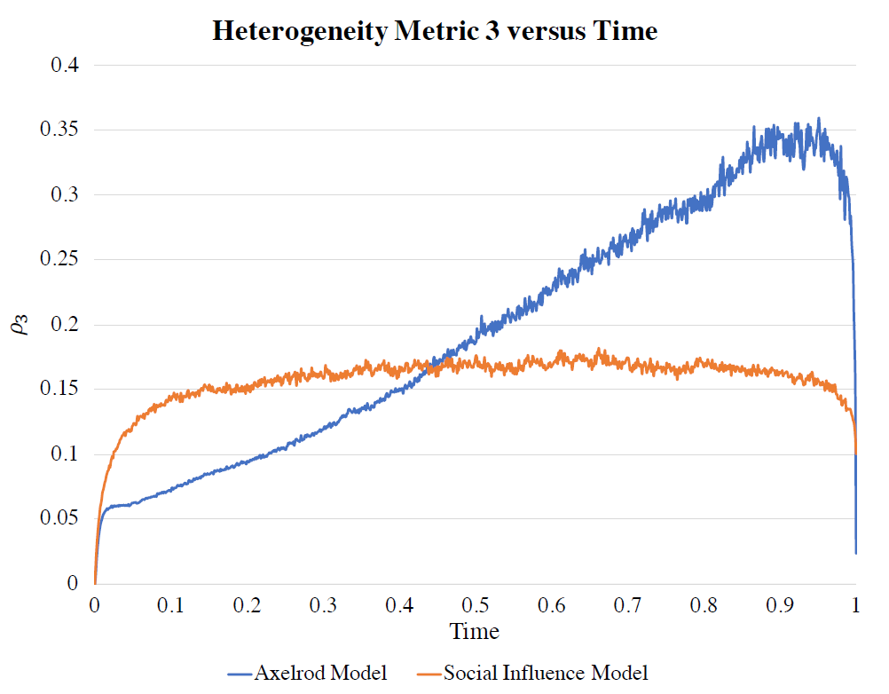
A different aspect of the system behavior is revealed by the geometrical metric \(\rho_3\), shown in Figure 14. For both models, the initial rapid rise of \(\rho_3\) from nearly zero is readily understood: When the system is initialized at the start of the simulation, all agents are assigned random trait values, meaning that there will be a large number of single-agent regions and zones (which are all perfectly square-shaped and smooth), and hence \(\rho_3\) starts off near zero. But as these regions and zones begin to interact, evolve, and merge, their shapes increasingly deviate from that of a square (via some combination of either coarsening of their boundaries and/or elongation), resulting in a growing value of \(\rho_3\). Following the initial rapid rise in \(\rho_3\), observe that the Social Influence Model plateaus whereas the Axelrod Model continues to steadily increase. This is consistent with the relatively rapid formation of robust zones in the former, compared to predominance of susceptible-to-change regions in the latter. An interesting new phenomena is revealed by metric \(\rho_3\) at the very end the simulations just before the systems freeze into an absorbing state. In both models one sees a rapid drop in the value of the metric, indicating that rough or filamentary regions and zones are being eliminated. However, this effect is strikingly more pronounced in the Axelrod Model (Figure 14). We can attribute this to the dominant-regions effect, in which small, non-compact regions are being quickly eaten by a large, dominant region; in the Social Influence Model this occurs to a much lesser extent owing to the higher prevalence of zones (compared to regions). A complementary insight4 is that the Axelrod model can be viewed as \(F\) coupled \(Q\)-state voter models without surface tension, whereas the interaction with the local field (all neighbors) in the Social Influence Model introduces surface tension. This would be expected to produce rougher boundaries in the Axelrod case and smoother ones in the Social Influence Model, which is consistent with the former’s higher peak value in Figure 14 prior to the collapse.
Conclusions
In conclusion, our model has allowed us to analyze the implications of local social influence in the dissemination of culture across a society, and has unveiled some interesting features. Most notable is the overall amplification of heterogeneity seen in the final absorbing state. In other words, the more one allows individual agents to be influenced by other agents in their local environment, the less homogeneous the resulting society becomes. The detailed, underlying mechanisms elucidated in this paper responsible for this counter-intuitive result can be qualitatively understood, at least in part, as follows: While caring about your neighbor’s opinions will initially make you more likely to assimilate your views to theirs, once you do so your opinions will be less likely to switch in the future since there is now a consensus belief in your local environment. In this manner, social influence produces a hardening of opinions within local zones that are relatively robust to external influences. However, as our simulations and analysis have revealed, the underlying dynamical mechanism responsible for this amplification of heterogeneity is both rich and nuanced. As shown, it involves a competition between the diffusion-based “dominant-regions” effect that promotes homogeneity through the absorption of small regions by larger ones, and a local social-influence effect that makes cultural zones (even small ones) more robust to infiltration by bordering regions. We remark that a related observation of enhancement of heterogeneity via social influence was previously noted in an interesting model developed by Flache & Macy (2011). Although the overall focus and implementation of neighborhood-based social influence in the model of Flache & Macy (2011) differs from the model studied here in multiple respects (e.g., the former incorporates selection error, “modal” traits, cultural perturbations, and a different social interaction scheme) – thereby making direct comparisons somewhat difficult – nonetheless there are strong parallels in the underlying mechanisms responsible for amplification of heterogeneity, suggesting that these social-influence-driven mechanisms must be fairly robust and likely do not depend too strongly on the details of the model.
Our analysis also sheds some modest new light on the inner dynamics of the original Axelrod Model, which incorporated the effects of homophily and assimilation but not the effects of collective local opinion as described here. In particular, while Axelrod pointed out that a zone could eventually be penetrated by a far-away region (through intermediary agents), and that there is a dominant-regions effect whereby big regions “eat” neighboring small regions, we have shown how the interplay between these two effects plays a critical dynamical role in the behavior of each model. In particular, in Axelrod’s model this interplay frequently leads to a convergence to a purely homogeneous state, whereas this interplay is significantly weakened by the introduction of a social influence factor into our model, making it difficult for distant regions to break large zones, leading to greater heterogeneity. Additionally, in our analysis we have numerically explored a two-dimensional version of Axelrod’s qualitative, one-dimensional diffusion argument as the basis of the dominant-regions effect. Lastly, our findings relating to lattice size and boundary effects (presented in greater detail in the Appendices below) expand our understanding of Axelrod’s original work in this regard. In particular, Axelrod noted how boundary effects became progressively less important as lattice size increases. However, this proves not always to be the case. In Figure 3, for instance, we noted how, in the Social Influence Model, the number of frozen zones appears to increase with lattice size (as opposed to the Axelrod model in which it saturates and then decreases). However, if we were to remove the boundary walls of the lattice by imposing doubly periodic boundary conditions (effectively wrapping the grid into a torus), we observe that the number of frozen zones in the Social Influence Model drops off significantly compared to the case with boundary walls (see Figure 16). This shows how boundary effects can still play an important role even in large systems.
Finally, in this work we also developed three novel heterogeneity metrics which, in addition to providing direct insights into the cultural dissemination process in our Social Influence Model and Axelrod’s original model, also have potential utility across a broad spectrum of cultural dissemination models in general. The first of these metrics examines the level of difference between neighboring agents; the second is an entropic measure that takes account of the numbers and sizes of the distinct regions and computes the level of configurational disorder in the system; the third provides direct information about the geometric qualities of the different region/zone shapes and quantifies how filamentary and/or rough they are (vs. being geometrically compact and smooth). This last metric, for example, revealed a previously unrecognized dynamical attribute of Axelrod’s original model - the rapid dissolution, compactification, and/or smoothening of small zones in the final stages of the cultural evolution - and also revealed how this effect is mitigated by the action of local social influence.
Model Documentation
The model was built in Python. The code is available at this link: https://www.comses.net/codebases/dda2d2ac-0cf9-46f6-a213-e0a9a30378ed/releases/1.0.0/.Notes
- The definitions of cultural regions and zones used here are not the same as those used in Axelrod’s original work (Axelrod 1997).
- Guided by the average number of events to reach the absorbing state.
- Fortunately, this kind of scenario occurs fairly frequently in our simulations, particularly once the system settles into an absorbing state.
- We thank an anonymous referee for this insight.
Appendix
A: A remark on the effect of the non-overlapping neighbors
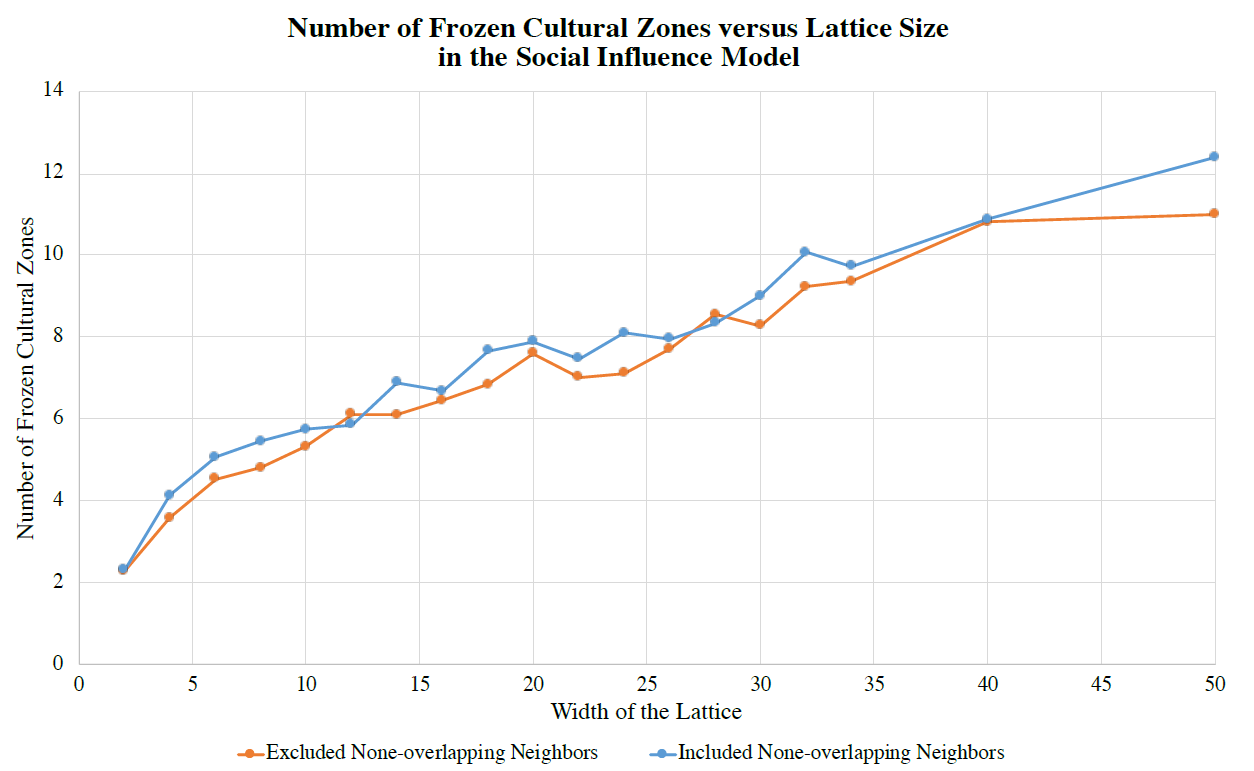
Recall that in our model the social influence of an agent’s neighbors took the form of a switching probability \(Q^f_{i,j}\) as described in Equation 7. In this construction, we note that neighbors whose trait values differed from that of both the selected agent and the selected neighbored did not factor into the calculation of the switching probability. The motivation for ignoring these “non-overlapping” neighbors was that they assumed the role of third-party candidates whose own trait values were irrelevant when directly deciding between the trait values \(\sigma_i^f\) and \(\sigma_j^f\) of the selected agent and neighbor. However, it is reasonable to consider the ramifications of including the non-overlapping neighbors, since their presence indicates a greater diversity of views within that local neighborhood, which in turn could conceivably enhance agent \(i\)’s willingness to switch its own trait values, at least to a certain extent. We can model this by introducing a modified switching probability \(Q'^f_{i,j}\) as follows:
| \[Q'^f_{i,j}=\frac{O_i(\sigma_j^f)+\frac{1}{2}\left[|N_i|-O_i(\sigma_j^f)-O_i(\sigma_i^f)\right]}{O_i(\sigma_i^f)+O_i(\sigma_j^f)+\frac{1}{2}\left[|N_i|-O_i(\sigma_j^f)-O_i(\sigma_i^f)\right]}, \] | \[(17)\] |
To explore the implications of this, we conducted a series of numerical simulations on the Social Influence Model using this modified switching probability \(Q'^f_{i,j}\). We found that the inclusion of these non-overlapping neighbors into the model yielded no significant qualitative changes in the model’s overall behavior. The only quantitative difference was a modest reduction in number of frozen zones compared to our original Social Influence Model - a result which could be readily anticipated given that \(Q'^f_{i,j} \geq Q^f_{i,j}\), meaning that the modification to the switching probability effectively reduces an agent’s resistance to change.
B: A remark on boundary conditions
In our standard model, agents’ neighbors only include those individuals directly adjacent to them. Most agents, being located in the interior of the lattice, will therefore have four immediate neighbors. However, agents along the boundaries of the square lattice will have fewer neighbors with whom to directly interact (i.e., corner agents only have two neighbors; agents on the boundary’s edge have three). Since boundary effects are known to influence dynamical evolution in cultural dissemination models (Axelrod 1997; LaBerge et al. 2020), it is important to understand, and potentially minimize, their impact. There are two natural means of mitigating such boundary effects. The first is to increase overall lattice size, which increases the proportion of interior agents to boundary agents. The second is to impose doubly periodic boundary conditions on the square lattice, thereby turning the square into a torus. While this latter method has the drawback of being topologically unrealistic, it nonetheless has two key virtues: uniformity, in that all agents have precisely four neighbors with whom to interact, and ease of numerical implementation, since it does not require using progressively larger lattice sizes. We examine both cases - varying both lattice size and boundary type (periodic vs. non-periodic) for both the Social Influence Model and Axelrod model. Results are illustrated in Figure 16.
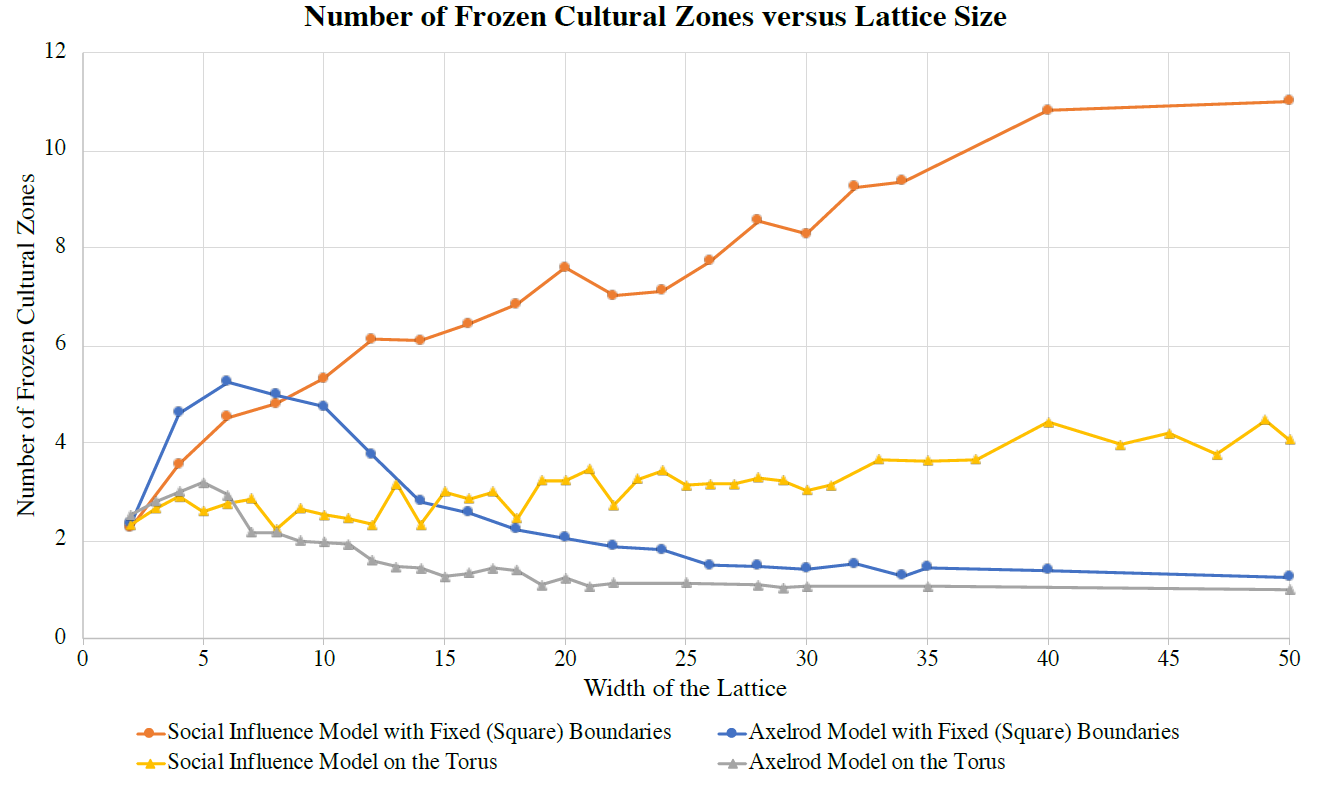
It is clear that in both the Social Influence Model and Axelrod Model the presence of fixed (square) boundaries enhances the formation of frozen zones - when these boundaries are removed through the introduction of periodic boundary conditions the number of frozen zones drops in both cases. This is as expected, since previous studies have elucidated the mechanism by which boundaries can increase heterogeneity (Axelrod 1997; LaBerge et al. 2020). More interesting is the overall behavior of the Social Influence Model with fixed boundary conditions versus periodic boundary conditions. Here we see that although the presence of periodic boundary conditions significantly curtails the growth in the number of frozen zones, nonetheless the total number of frozen zones in the periodic boundary case continues to slowly increase with lattice size (unlike the Axelrod model). We can understand this as follows: As argued earlier (see Section “Heterogeneity and Lattice Size”), although the dominant-regions effect for large lattice sizes is in operation in both the Social Influence Model and Axelrod model, in the former model the agents in more distant regions are less able to propagate their cultural traits in order to break zones. The resulting robustness of zones leads to a higher total number of frozen zones in the absorbing state. Hence, for the Social Influence Model with fixed boundaries, the number of frozen zones will increase with lattice size. With periodic boundaries, the same general phenomena is occurring, but now the dominant-regions effect is enhanced by the lack of boundaries because large regions are now free to expand in all directions, no longer being confined by rigid boundary walls. However, while this lowers the overall number of frozen zones compared to the rigid boundary case, it is still not sufficient to prevent an overall increase in the number of frozen zones with increasing with lattice size since distant regions still cannot propagate their traits efficiently enough to break zones.
C: Order-disorder phase transition
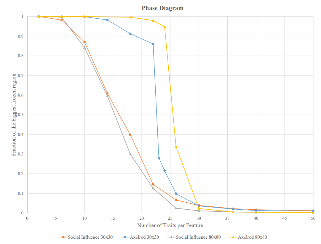
In Figure 3, we directly compared lattice-size effects in the Axelrod and Social Influence models for the same parameter values (\(F=5\) and \(Q=10\)) and noted qualitatively distinct behaviors. It is known from the work of Castellano et al. (2000) and Klemm et al. (2003) that certain cultural dissemination models are capable of exhibiting order-disorder phase transitions. In particular, Castellano et al. (2000) showed that in the Axelrod model there is a first-order, discontinuous phase transition whenever \(F >2\). Although somewhat peripheral to our main study, we numerically reproduce here this phase transition (for the case \(F=5\)) for the Axelrod Model, and then directly compare its behavior to that of the Social Influence Model taken at the same parameter value \(F=5\). Our results are shown in Figure 17. As seen from the figure, for the Axelrod model there is a discontinuous transition in the limit of large system size, wherein for small numbers of traits \(Q\) the absorbing state is in an “ordered” phase in which there is a single, dominant frozen zone that subsumes most of the lattice, while in the disordered phase (higher \(Q\)) no such dominant frozen zone exists. In contrast, for the Social Influence Model at \(F=5\) there does not exist a corresponding discontinous (first-order) transition. Importantly, for purposes of our investigation, we intentionally always make the direct comparison between the two models’ behaviors at the same parameter values so as to isolate the effects of the social influence factor under the same conditions (since our focus is on analyzing the dynamical processes leading to zonal formation in the two models when their underlying structure \((F,Q)\) is identical). And as noted previously, at \((F,Q)=(5,10)\) we see from Figure 3 an intrinsic difference between the two models in the growth in the overall numbers of frozen zones with lattice size (associated with the presence/absence of a social influence factor), as explained by the mechanisms described in Section 3.8. Nonetheless, an ancillary yet highly interesting issue (albeit outside the scope of the present work) remains – namely, whether or not the Social Influence Model can also display discontinuous phase transitions at other parameter choices, and moreover, whether it might be possible to somehow map the Social Influence Model onto the Axelrod Model by appropriately rescaling the parameter values (which in turn might perhaps even allow one to identify certain universal features common to both models, such as scaling exponents). This is left for future investigation.
D: Increase in neighborhood size
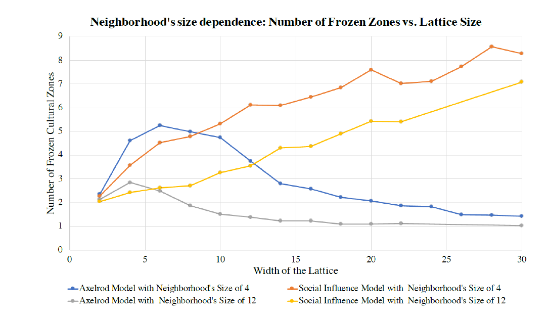
In the Axelrod Model, it is known that an increase in neighborhood size tends to decrease the overall number of frozen regions. The introduction of a social-influence factor into the model would not be expected to alter the mechanism responsible for this behavior. As a test, we increased the neighborhood size from four to twelve in the models and reproduced Figure 3; see Figure 18. Although we see the expected decrease in overall numbers of frozen zones, the same qualitative trends prevailed.
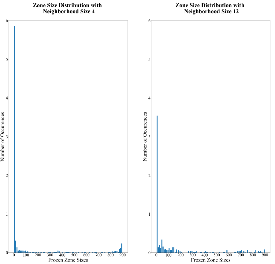
Figure 19 shows the distribution of zone sizes for the original neighborhood size (4) and the expanded neighborhood size (12). For the expanded neighborhood, observe that there are fewer frozen zones per run on average compared to the smaller neighborhood. Moreover, an expanded neighborhood leads to a higher occurrence of moderate-size zones (e.g., of sizes 20-200).
E: Amplification of heterogeneity in other models with Social influence
In our Social Influence Model we observed (see Figures 3 and 6) a marked increase in diversity compared to the original Axelrod model owing to the introduction of a neighborhood-based social-influence factor into our model. It is interesting to test how sensitive this finding is to the details of the particular social-influence factor we used. Towards this end, we numerically examined the corresponding behavior in an earlier social-influence-type model first studied by Flache & Macy (2011). In order to make this comparison, we first stripped down the Flache & Macy (2011) model by removing a perturbative component in the model that allowed it to evolve indefinitely. By removing this component, an absorbing state can be reached and the number of frozen zones counted. Flache & Macy (2011) anticipated that there should be an increase in heterogeneity associated with their social-influence factor. We confirmed this finding - see Figure 20 - but observed some features which warrant discussion. Most notably, a comparison of Figure 20 with Figure 3 shows that the while both models exhibit similar qualitative amplification of heterogeneity with lattice size, the actual number of frozen zones in the Flache & Macy (2011) model is manyfold larger. We believe this can be traced to an essential difference in how social influence is incorporated into each model. In our Social Influence Model, the algorithm is such that the system will always evolve into an absorbing state in which the agents in a given frozen zone never share any trait values in common with agents in a neighboring frozen zone. However, in the Flache & Macy (2011) scheme, the social-influence algorithm employed uses a type of minimum-threshold update rule. This in turn means that once an absorbing state is reached, it is possible that the agents in one frozen zone may still have a trait value for a given feature which is the same at that of an agent in an adjacent frozen zone. Owing to this possibility of ‘trait overlap’ between frozen zones, the resulting total number of frozen zones in this case is notably larger than in the Social Influence Model. Despite these quantitative differences, however, we emphasize that both social-influence schemes produce an increase in diversity with lattice size, suggesting that despite quantitative differences, the underlying qualitative mechanism promoting diversification operates similarly in both systems.
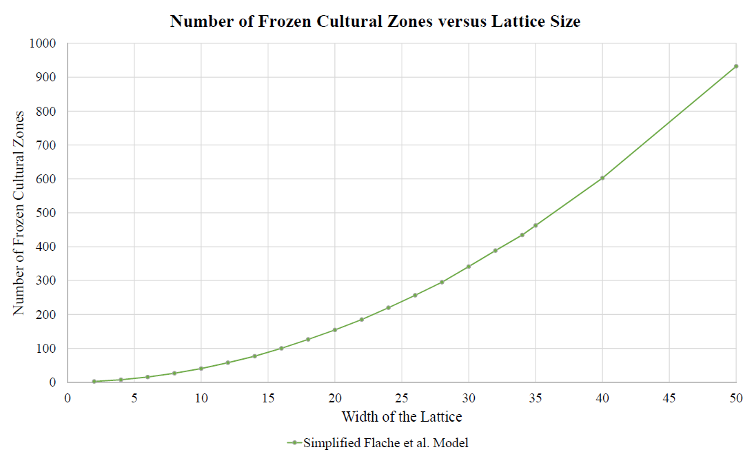
F: Lattice size effects for other parameter choices
As noted in Table 2, there is an overall amplification of diversity associated with social influence for a variety of different parameter \((F,Q)\) choices in comparison to the Axelrod Model (save for parameter choices producing a monocultural absorbing state). Figure 3 in the main paper, taken at \((F,Q)=(5,10)\), illustrates the interplay between amplification and lattice size. Figure 21 illustrates analogous behavior at a different parameter choice, \((F,Q)=(7,15)\).
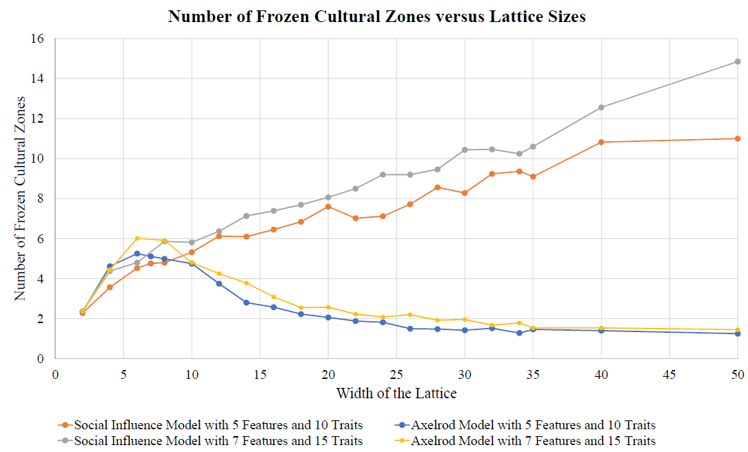
References
ABELSON, R. P. (1964). 'Mathematical models of the distribution of attitudes under controversy.' In N. Frederiksen & H. Gulliksen (Eds.), Contributions to Mathematical Psychology. New York, NY: Rinehart Winston.
ANDERSON, B. (1991). Imagined Communities: Reflections on the Origin and Spread of Nationalism. New York, NY: Verso Books.
AXELROD, R. (1997). The dissemination of culture: A model with local convergence and global polarization. Journal of Conflict Resolution, 41(2), 203–226. [doi:10.1177/0022002797041002001]
AXELROD, R. (2006). 'Agent-based modelling as a bridge between disciplines.' In L. Tesfatsion & K. L. Judd (Eds.), Handbook of Computational Economics: Agent-Based Computational Economics (Vol. 2, pp. 1565–1584). Amsterdam: North Holland. [doi:10.1016/s1574-0021(05)02033-2]
AXELROD, R., & Bennett, S. D. (1993). A landscape theory of aggregation. British Journal of Political Science, 23(2), 211–233. [doi:10.1017/s000712340000973x]
BALLAS, D., Clarke, G., & Wiemers, E. (2005). Building a dynamic spatial microsimulation model for ireland. Population, Space and Place, 11(3), 157–172. [doi:10.1002/psp.359]
BARROS, J. (2012). 'Exploring urban dynamics in Latin American cities using an agent-based modelling approach.' In A. J. Heppenstall, A. Crooks, L. M. See, & M. Batty (Eds.), Agent-Based Models of Geographical Systems (pp. 571–589). Berlin Heidelberg: Springer. [doi:10.1007/978-90-481-8927-4_28]
CASTELLANO, C., Fortunato, S., & Loreto, V. (2009). Statistical physics of social dynamics. Review of Modern Physics, 81(591). [doi:10.1103/revmodphys.81.591]
CASTELLANO, C., Marsili, M., & Vespignani, A. (2000). Nonequilibrium phase transition in a model for social influence. Physical Review Letters, 85(16), 3536–3539. [doi:10.1103/physrevlett.85.3536]
DALEY, D. J., & Kendall, D. G. (1964). Epidemics and rumors. Nature, 204(1118).
DEFFUANT, G., Neau, D., Amblard, F., & Weisbuch, G. (2000). Mixing beliefs among interacting agents. Advances in Complex Systems, 3(1), 87–98. [doi:10.1142/s0219525900000078]
FLACHE, A., & Macy, M. W. (2011). Local convergence and global diversity: From interpersonal to social influence. Journal of Conflict Resolution, 55(6). [doi:10.1177/0022002711414371]
FRIEDKIN, N., & Johnsen, E. (2011). Social Influence Network Theory: A Sociological Examination of Small Group Dynamics. Cambridge, MA: Cambridge University Press. [doi:10.1017/cbo9780511976735]
GANDICA, Y., Medina, E., & I., B. (2013). A thermodynamic counterpart of the Axelrod model of social influence: The one-dimensional case. Physica A: Statistical Mechanics and Its Applications, 392(24), 6561–6570. [doi:10.1016/j.physa.2013.08.033]
HEGSELMANN, R., & Krause, U. (2002). Opinion dynamics and bounded confidence. Journal of Artifical Societies and Social Simulation, 5(3), 2: https://www.jasss.org/5/3/2.html.
HEPPENSTALL, A. J., Evans, A. J., & Birkin, M. H. (2006). Using hybrid agent-Based systems to model spatially-Influenced retail markets. Journal of Artifical Societies and Social Simulation, 3(9), 2: https://www.jasss.org/3/9/2.html.
JAYNES, E. T. (1978). 'Where do we stand on maximum entropy?' In R. D. Rosenkrantz (Ed.), E. T. Jaynes: Papers on Probability, Statistics and Statistical Physics. Berlin Heidelberg: Springer. [doi:10.1007/978-94-009-6581-2_10]
KEIJZER, M. A. (2018). Communication in online social networks fosters cultural isolation. Complexity, 2018. [doi:10.1155/2018/9502872]
KLEMM, K., Eguíluz, V. M., Toral, R., & San Miguel, M. (2003). Global culture: A noise-induced transition in finite systems. Physical Review E, 67(045101). [doi:10.1103/physreve.67.045101]
KOHLER, T. A., Kresl, J., Van Wes, Q., Carr, E., & Wilshusen, R. H. (2000). 'Be there then: A modeling approach to settlement determinants and spatial efficiency among late ancestral Pueblo populations of the Mesa Verde Region, U.S. Southwest.' In T. A. Kohler & G. J. Gumerman (Eds.), Dynamics in Human and Primate Societies: Agent-Based Modeling of Social and Spatial Processes. Oxford: Oxford University Press. [doi:10.1093/oso/9780195131673.003.0012]
KUPERMAN, M. N. (2006). Cultural propagation on social networks. Physical Review E, 73(4).
LABERGE, N., Chaderjian, A., Ginelli, V., Jebsen, M., & Landsberg, A. (2020). Modeling cultural dissemination and divergence between rural and urban regions. Journal of Artificial Societies and Social Simulation, 23(4), 3: https://www.jasss.org/23/4/3.html. [doi:10.18564/jasss.4391]
PARISI, D., Cecconi, F., & Natale, F. (2003). Cultural change in spatial environments: The role of cultural assimilation and internal changes in cultures. Journal of Conflict Resolution, 47(2), 163–179. [doi:10.1177/0022002702251025]
PERES, L. R., & Fontanari, J. F. (2012). Effect of external fields in Axelrod’s model of social dynamics. Physical Review E, 86(031131). [doi:10.1103/physreve.86.031131]
PFAU, J., Kirley, M., & Kashima, Y. (2013). The Co-evolution of cultures, social network communities, and agent locations in an extension of Axelrod’s model of cultural dissemination. Physica A: Statistical Mechanics and Its Applications, 392(2), 381–391. [doi:10.1016/j.physa.2012.09.004]
REIA, S. M., & Fontanari, J. F. (2016). Effect of long-range interactions on the phase transition of Axelrod’s model. Physical Review E, 94(052149). [doi:10.1103/physreve.94.052149]
RODRÍGUEZ, A., del Castillo, M., & Vázquez, G. J. (2009). Induced monoculture in Axelrod model with clever mass media. International Journal of Modern Physics C, 20(8), 1233–1245. [doi:10.1142/s012918310901431x]
SCHELLING, T. C. (1971). Dynamic models of segregation. Journal of Mathematical Sociology, 1, 143–186.
SHIBANAI, Y., Yasuno, S., & Ishiguro, I. (2001). Effects of global information feedback on diversity: Extensions to Axelrod’s adaptive culture model. Journal of Conflict Resolution, 45(1), 80–96. [doi:10.1177/0022002701045001004]
STIVALA, A., & Keeler, P. (2016). Another phase transition in the Axelrod model. arXiv preprint. Available at:https://arxiv.org/abs/1612.02537.
TOFFOLI, T., & Margolus, N. (1987). Cellular Automata Machines: A New Environment for Modeling. Cambridge, MA: MIT Press. [doi:10.7551/mitpress/1763.001.0001]
VAZQUEZ, F., Castelló, X., & San Miguel, M. (2010). Agent based models of language competition: Macroscopic descriptions and order-Disorder transitions. Journal of Statistical Mechanics Theory and Experiment, 2010(4), P04007. [doi:10.1088/1742-5468/2010/04/p04007]