
Introduction
In light of contemporary and historical events, it is evident that there exist some striking cultural discrepancies between urban and rural communities. This urban-rural divergence is manifest in many present-day contexts, e.g. in an examination of political beliefs and voter preferences across the United States (Kron 2012); in television viewing habits (Katz 2016); in perceptions of fairness and equity regarding federal assistance (Del Real 2017); in educational expectations (Andres & Looker 2001); in leisure-time physical activity (Wilcox et al. 2000), in levels of reported religiosity (Lyons 2003), etc. Moreover, the levels of cultural homogeneity/heterogeneity found within rural regions and urban regions can also markedly differ.
What are the underlying reasons for the emergence of these cultural distinctions between urban and rural communities? Clearly the apposite factors are myriad and intertwined, involving a complex mixture of social, historical, demographic, economic, and political forces and interactions. Indeed, with so many conflating factors, isolating and understanding even some of the most basic of these factors influencing rural-urban cultural development can be challenging. To make headway into this labyrinthine question, we adopt a reductionist approach inspired by Axelrod’s seminal work (1997) on cultural dissemination, which allows us to strategically circumvent some of these complexities and significantly refine this question. Towards this end, we will employ an agent-based, computational network model of cultural dissemination to isolate and examine the effect of one of the most fundamental, core influences on rural-urban cultural evolution — the different population densities in urban vs. rural regions. In particular, what intrinsic effect does the higher population density of urban regions compared to rural regions have on their subsequent cultural developments, and, most interestingly, how is the development in each region mutually influenced by the other? Remarkably, basic answers to these seemingly elementary questions have yet to fully emerge, and much remains uncharted. This is the issue we seek to address in this work.
We subdivide the issue of population density and its implications for rural-urban cultural dissemination into two core components:
- Range of interactions with neighbors, i.e., owing to higher population density, urbanites generally have a greater number of geographically accessible neighbors with whom to potentially interact
- Frequency of interactions with neighbors, i.e., owing to higher population density, urbanites will typically have more frequent opportunities to interact with their neighbors than their rural counterparts.
As will be seen, the difference in rural-urban population density proves to have a pronounced effect on the overall level of cultural homogeneity or heterogeneity that emerges in each of the two regions. Our study will articulate how each of the two primary factors — the range and the frequency of interactions with neighbors — contribute to and/or impact the level of cultural homogeneity/heterogeneity that develops in urban regions compared to rural regions.
Stepping back for a moment, we note that the general study of “culture” — defined as a set of characteristics which may be influenced by social interactions — has been the focus of a great deal of computational study. Robert Axelrod’s seminal Adaptive Culture Model (ACM) sought to create a computational model to answer the question: “If people tend to become more alike in their beliefs, attitudes, and behavior when they interact, why do not all such differences eventually disappear?” (Axelrod 1997). Axelrod’s model is based on two basic principles: (1) that two individuals are more likely to interact the more similar they are (“homophily”), and (2) that when two individuals interact they tend to become more similar (“assimilation”). Interestingly, this early model demonstrated that even when social interactions are governed strictly by homophily and assimilation — both of which would seemingly conspire to produce a homogeneous society — nonetheless cultural heterogeneity/polarization can persist.
Many studies have since modified the ACM to model various contemporary, real-world phenomenon. Teams have studied cultural drift by applying cultural perturbations of varying frequencies to the ACM (Klemm et al. 2003b) and by introducing network homophily (Centola et al. 2007), while others have adapted the ACM to study the effects of global information feedback on a population’s cultural diversity by introducing mass media as an influence on the model’s agents (Shibanai et al. 2001; González-Avella 2007; Rodríguez et al. 2010). Perhaps most relevant to our study is J. Michael Greig’s work (Greig 2002) in which the effects of globalization are studied through the extension of agents’ neighborhood sizes. Greig, like Axelrod, finds that expanding neighborhood size in a society results in cultural homogeneity. Greig notes that with larger neighborhoods, the initial random cultural attributes that are most prevalent at the start of the ACM simulation become less dominant when the system settles. Additional contributions have identified and characterized a nonequilibrium phase transition in the ACM that separates states of cultural homogeneity from cultural fragmentation (Castellano et al. 2000; Klemm et al. 2003b) and have made insights into the process of community formation across varying network structures for the ACM (San Miguel et al. 2005) and for multi-agent systems more broadly (Xie et al. 2014; Cai et al. 2017).
Our study models a society in which there are distinct ‘urban’ and ‘rural’ regions, wherein the agents in an urban geography are assumed to have more neighbors than their rural counterparts and to potentially interact more frequently with those neighbors. Apart from these two geographically based differences, no other inherent distinctions between urban and rural agents are assumed. In this manner, we are able to isolate the effects of the frequency of interactions with neighbors and the range of interaction with neighbors, without being subsumed by a host of other relevant but conflating factors affecting rural-urban development such as migration, local demographics, etc. As will be discussed in detail, our central findings are that increasing the neighborhood range within an urban region leads to increased cultural homogeneity everywhere (i.e., in both the urban and rural regions), but, rather unexpectedly, increasing the frequency of interactions within an urban region produces more homogeneity within the urban region but less homogeneity in the rural region. These effects result from the cultural interactions between urban and rural regions as they develop, and cannot be understood simply by examining each region in isolation from the other.
Background: Adaptive Cultural Model
We begin by briefly recalling the basic attributes of the original ACM, and then show how to repurpose it to address our central thematic questions regarding the emergence of rural-urban differences.
The standard ACM (Axelrod 1997) consists of a two-dimensional grid with each node representing an agent. Culture is encapsulated in this model via a set of “features” representing the characteristics that agents possess which can be influenced by others through social interactions (e.g., political leaning, religious affiliation, favorite genre of movie, etc.). For each feature, “traits” refer to the specific values that the given feature can take on (e.g., for the feature Political Leaning, possible traits might include Conservative=1, Liberal=2, Moderate=3). Thus, if there are \(F\) features and each feature has q possible traits, then the current (cultural) state of any given agent can be numerically represented by a sequence of \(F\) integers, with each integer having a value (trait) in the range 1 to \(q\). At the start of the simulation, each agent in the grid is randomly assigned a set of trait values. At each subsequent timestep, one agent is selected at random (the “active” agent). One of the active agent’s neighbors is then randomly selected as a potential interaction partner. (In a 2-dimensional square grid, each agent except those on the boundaries has 4 nearest neighbors. This definition of “neighbor” though can be readily expanded as needed.) Whether the active agent and its selected neighbor actually interact or not is determined probabilistically based on the degree of cultural similarity between the two agents, as defined by the fraction of traits that the two share (e.g., if \(F = 5\) and the agent shares three traits in common with the selected neighbor, then there is a 3/5 probability that the two agents interact). Thus, the more similar two agents are, the higher their probability of interacting. If an interaction does take place, the active agent will (randomly) adopt one of this neighboring agent’s traits, making the two agents even more similar. Once the interaction is complete (or if the interaction did not occur in the first place), a new active agent is randomly selected and the entire process repeats. The simulation ceases when the entire grid of agents eventually reaches a stable configuration. In this absorbing state, no further changes occur, since every agent is now either culturally identical to a neighbor (i.e., shares all the same traits) or has zero traits in common with a neighbor. The number of distinct geographical cultural regions (stable regions) in this absorbing state is then counted to determine the degree of cultural homogeneity of this society of agents. The greater the number of distinct stable regions the more culturally diverse the society is. One of the most interesting aspects of Axelrod’s model is the existence of multiple distinct stable regions in the absorbing state despite the underlying homogenizing forces of assimilation and homophily.
The Rural-Urban Model
Our rural-urban model adapts Axelrod’s original ACM in order to analyze how culture disseminates differently in urban and rural areas, and, most critically, the interplay between the two. We first geographically divide the grid into urban and rural regions, and assume, by definition, that people living in urban areas will generally (1) have more frequent encounters with neighbors and (2) have a greater number of neighbors, than individuals living in a rural area. In the model, we then vary the relative frequency of these interactions and the range of these interactions, and thereby explore the resulting societal effects on the urban and rural regions. As in the ACM, the number of stable regions is used as the primary metric for characterizing the degree of cultural heterogeneity. Unlike Axelrod’s and more recent studies of cultural dissemination, however, our study is specifically designed to elucidate the interplay between urban and rural regions, and in particular to analyze how the underlying differences in interaction frequency and interaction range contribute to the emergence of cultural differences in social networks.
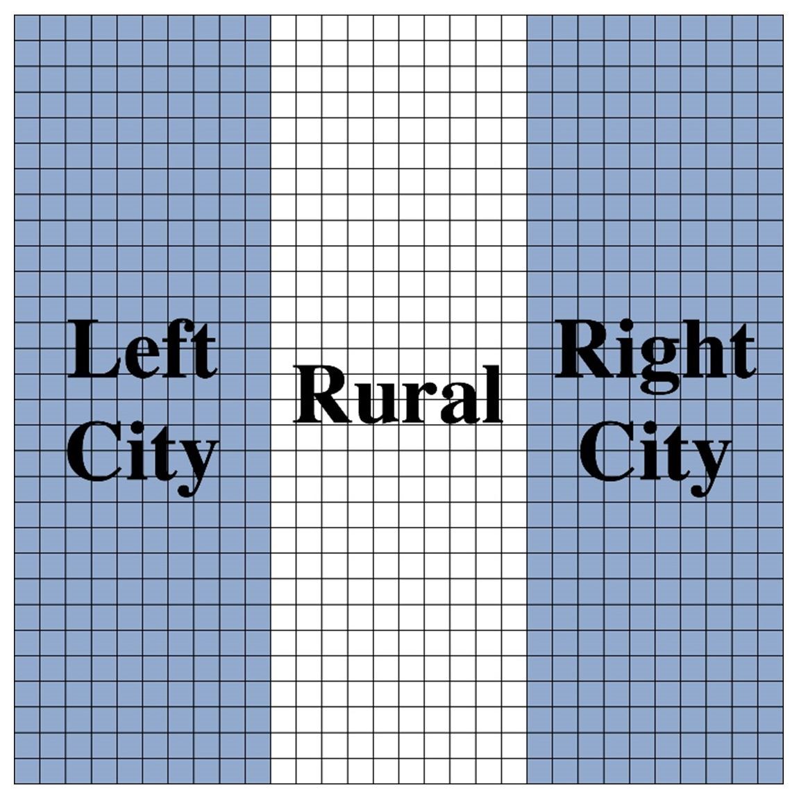
Our model can be visualized as a 30-by-30 grid where each node represents an agent; there are 900 agents in total. We divide our model into three regions as shown in Figure 1. The white region in the middle represents a rural region, while the blue regions on either side represent the urban (aka “city”) regions. We will refer to the left city area as \(C_L\), the rural area as R, and the right city as \(C_R\). We chose to assign each agent 5 features, where each feature could take on 15 trait values, as we found these parameters resulted in significant heterogeneity in the original ACM.
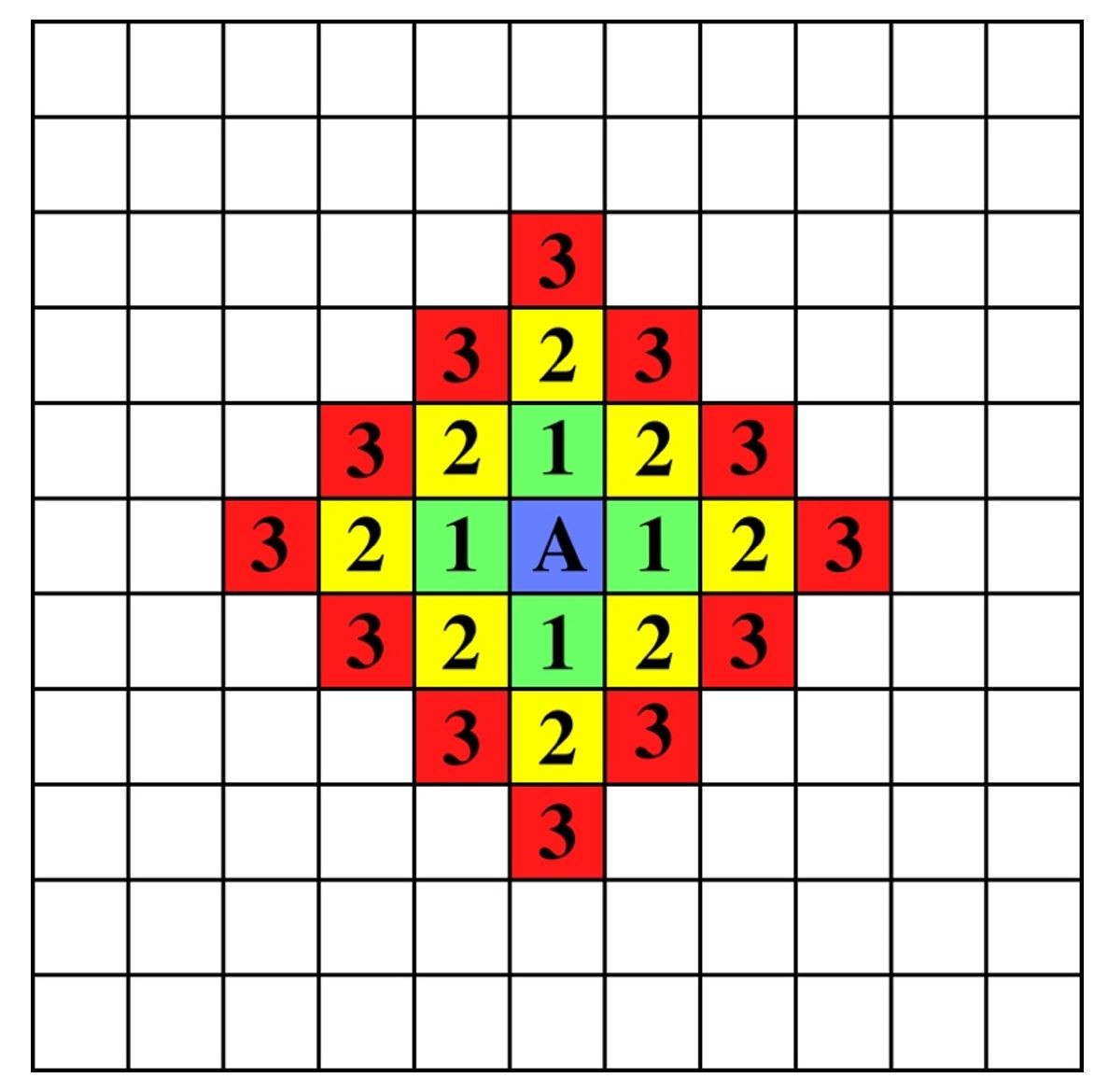
In the model, we will control the interaction range in the urban areas by varying the effective neighborhood sizes, \(n ≥ 1\), of the urban agents, while holding the neighborhood sizes of the rural agents fixed at 1. Selecting neighborhood sizes \(n > 1\) for the urban agents reflects the higher relative population densities of the cities. More specifically, neighborhood size n is defined using the standard taxicab metric (i.e., \(L_1\) norm): In the base case \(n = 1\), all urban agents in the grid have four immediate neighbors to the North, South, East and West with whom they can interact (just like the rural agents). For \(n = 2\), a given urban agent is able to interact with the 12 neighboring agents that lie within two lattice units away. For \(n = 3\), a given urban agent will have 24 neighbors, etc. See Figure 2 for a depiction of neighborhood sizes.
There are two modest qualifications to the above definition of neighborhood size. First, agents which lie close to the edge of the lattice may not have their full complement of neighbors. However, as described by Axelrod (1997), the potential impact of this edge effect is mitigated by the unidirectional nature of the model’s agent-agent interactions, since, by design, an active agent can take on a trait of its neighbor but the reverse interaction is not allowed. Second, to prevent city culture from artificially bleeding into the rural region as we increase the urban neighborhood size \(n\), we will impose a ‘nonporous’ boundary condition on the city-rural borders, i.e., an urban agent’s neighborhood is not permitted to extend more than one unit deep into the rural region regardless of how large \(n\) is set. For future reference, observe that, together, the agents and their neighborhoods form a graph, where the nodes of the graph correspond to the agents and the edges of the graph indicate whether two agents lie in the same neighborhood.
In our model, we can adjust the interaction frequency of the urban agents (relative to that of the rural agents) by choosing the agent-agent interaction probabilities appropriately. Specifically, during the simulations, when randomly selecting active sites, we can set the probability of choosing an active site in the two city regions \(C_L\), \(C_R\) to be higher than that of choosing an active site in the rural region \(R\). In this manner, agents in the urban regions will interact more frequently with their neighbors on average than rural agents will with theirs. For bookkeeping purposes, the different interaction frequencies will be reported as \(C_L:R:C_R\) ratios. For example, 2:1:2 denotes the condition that a given agent in either \(C_L\) or \(C_R\) is twice as likely to be randomly selected as the active agent than an agent in the rural region \(R\).
By independently adjusting the interaction frequency \(C_L:R:C_R\) and interaction range \(n\), we can examine each of these two factors in isolation as well as explore the interplay between the two. We note that setting the frequency ratio to 1:1:1 with neighborhood size \(n=1\) corresponds to the baseline case where the intrinsic distinctions between the ‘urban’ and ‘rural’ agents altogether vanish, and the model reduces to the original ACM. However, it is important to recognize that even in this case wherein the dynamical rules governing individual urban and rural agents are identical, certain regional differences can still emerge since a higher fraction of the urban agents lie near the edge of the lattice than do the rural agents. The potential implications of this will be discussed later.
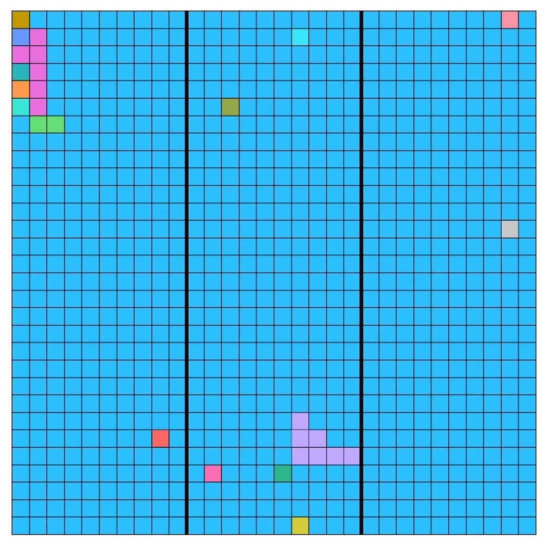
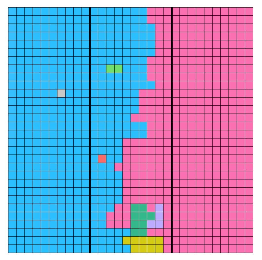
At the start of each simulation, we initialize the lattice by randomly assigning a set of trait values to each agent (via a uniform, i.i.d. probability distribution). Once a final absorbing state is achieved, we compute the average number of distinct cultural regions (aka “stable regions”) within each of the three areas, \(C_L, R, C_R\), as the standard metric for cultural diversity. Here, a ‘cultural region’ is defined as a set of agents which (i) have identical cultural states, and (ii) constitute a connected component in the graph theoretic sense (i.e., informally, a cultural/stable region is simply a patch of identical agents that are neighbors of one another). Cultural regions that span two or more of the three areas (\(C_L, R, C_R\)) are split and weighted proportionally to each area based on the fraction of its agents inside the area. In all trials in the simulations, there emerges a background “dominant culture” which permeates the entire lattice and comprises most of the agents. This dominant culture is not counted as belonging to any of the three areas \(C_L, R, C_R\) and is excluded from the overall count of the number of cultural regions. An example of an absorbing state of the grid with various stable regions is shown in Figure 3.
Results and Discussion
Interaction range
In our simulation, we first examine the potential impact of adjusting the interaction ranges of the city vs. rural agents on cultural diversity. We conducted a series of simulations on a 30x30 grid in which the neighborhood size (\(n\)) of the city agents was increased from \(n=1\) to \(n=5\), while keeping the neighborhood size of the rural agents fixed at \(n=1\). For each neighborhood size, we ran 100 trials and report the average number of stable regions and standard error once an absorbing state is reached. In all cases, the number of features was set to \(F=5\) and the number of traits per feature to \(q=15\), since this proved to be an interesting parameter set in the original ACM. Our results are shown in Figure 4.
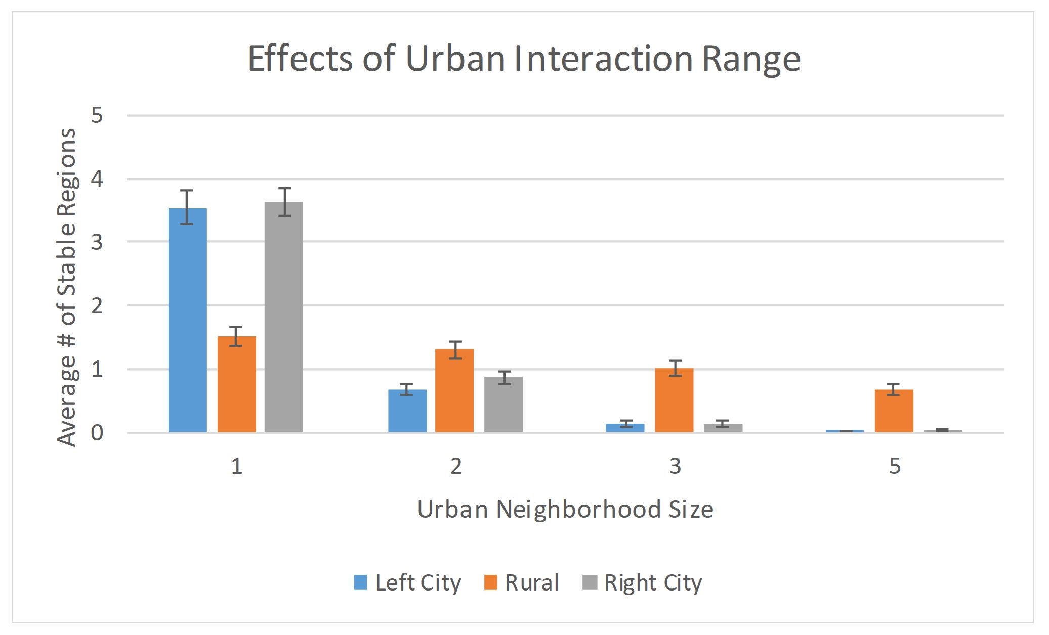
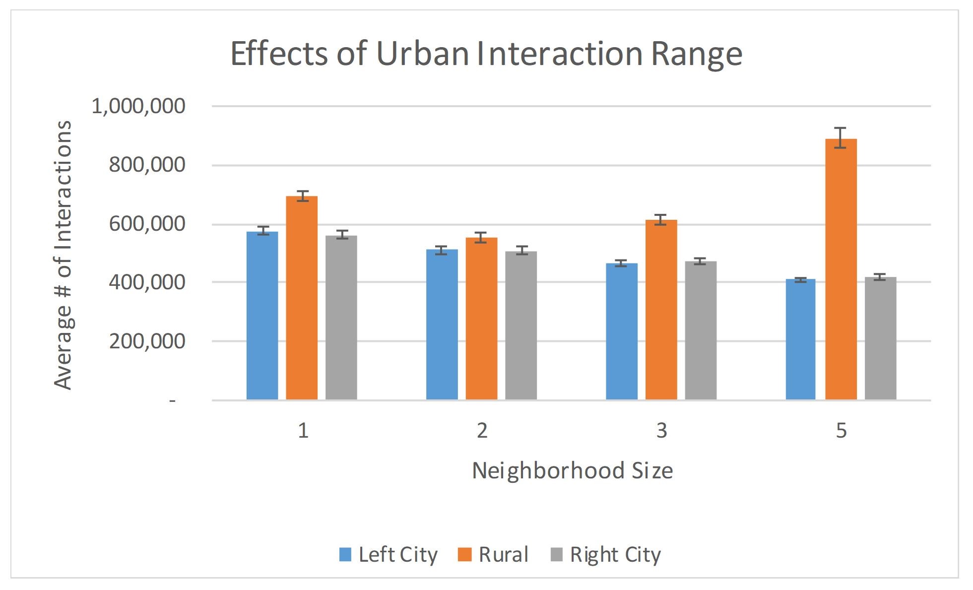
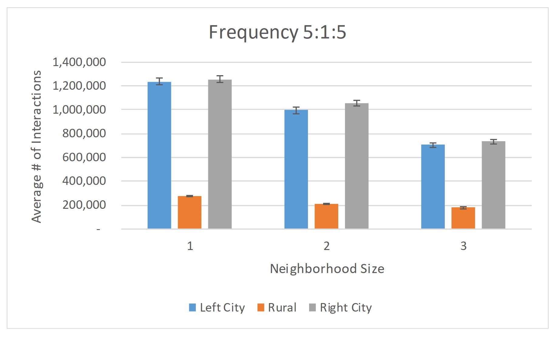
Several comments are in order. First, we observe that as the interaction range of the urban agents is increased, there is a dramatic reduction in number of distinct cultural regions within the cities, i.e., the cities are becoming increasingly homogeneous as the urban agents’ neighborhood size increases. This finding is perhaps not unexpected, being congruous with an analogous occurrence in Axelrod’s original ACM. In particular, in the ACM, when neighborhood sizes were increased throughout a uniform grid of agents (wherein there is no distinction between different types of agents), it was found that “larger neighborhoods result in fewer stable regions… Thus, when interactions can occur at greater distances, cultural convergence is easier” (Axelrod 1997). In our model, we observe a similar result — expanding the neighborhood size in the urban regions markedly enhances the model’s homogenizing tendency within those regions. Somewhat more interestingly, in Figure 4 we see that, despite the rural neighborhood size being held constant, expansion of the urban interaction range also leads to an increase in homogeneity in the rural region (i.e., fewer stable regions), albeit this tendency is less pronounced. We posit that what is occurring here is that the increased urban neighborhood size promotes more interactions within the rural region, which in turn allows the rural agents extended opportunities to interact amongst themselves, leading to greater homogenization. This hypothesis is supported by our related finding (see Figure 5) that the average number of interactions in the rural region increases significantly as the urban interaction range is extended.
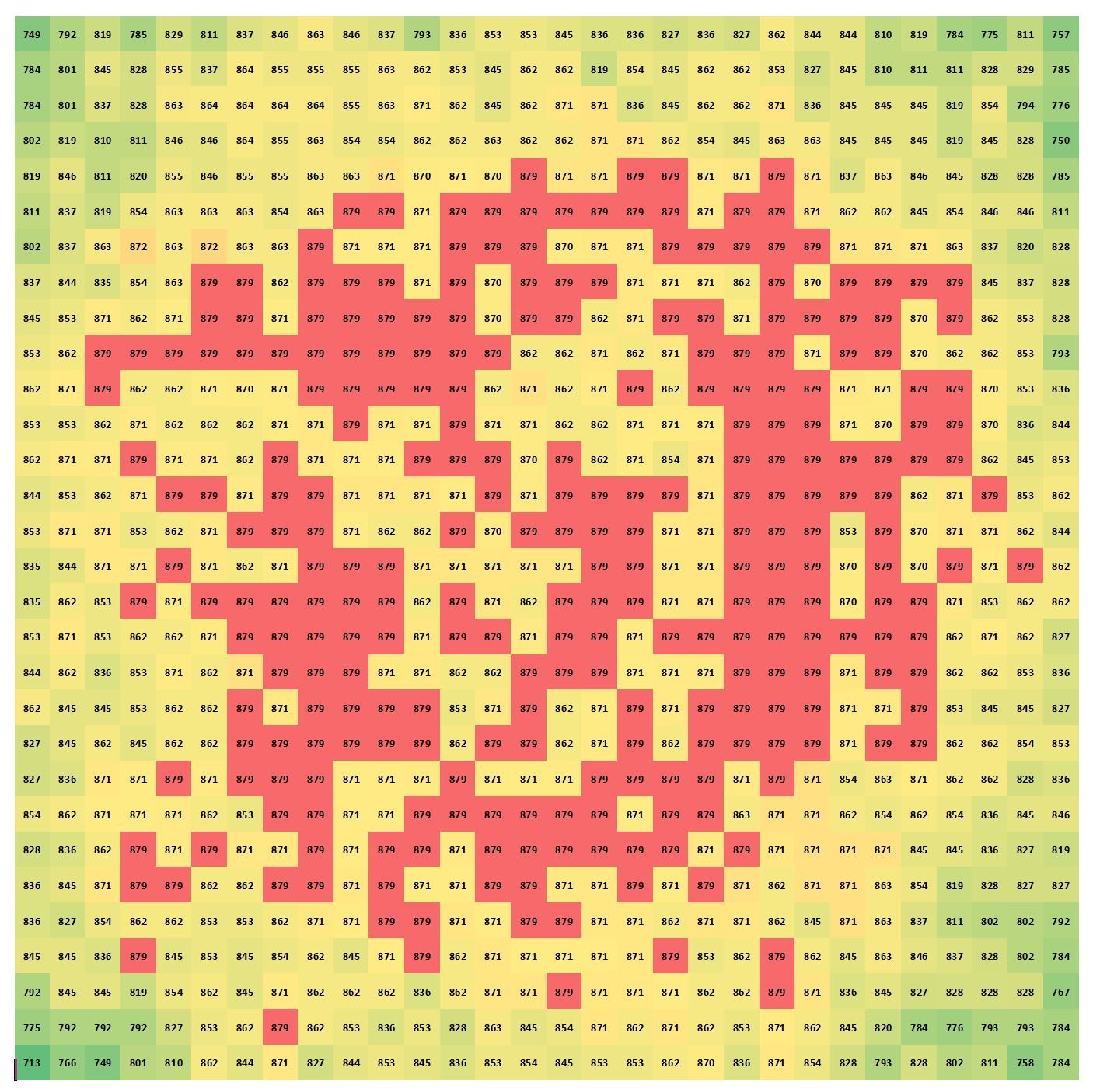
From Figure 4, we also observe an apparent disparity between the urban and rural regions for neighborhood size \(n=1\), where it is seen that the city regions display decidedly more heterogeneity than the rural region. At first blush it might seem surprising that any such differences between the urban and rural regions would exist, given that in this case (\(n=1\) with frequency 1:1:1) the interaction rules for the urban and rural agents are in fact identical. This interesting discrepancy can be understood as follows: While the agent-agent interaction rules are indeed identical in this case, observe that the two city regions have more sites that lie on the boundary of the lattice. Simulations show, however, that boundary effects tend to increase diversity in the vicinity of the boundary, which explains why the city and rural regions display different degrees of cultural diversity even when the neighborhood sizes \(n=1\) are identical. Figure 6 illustrates this boundary effect.
Interaction frequency
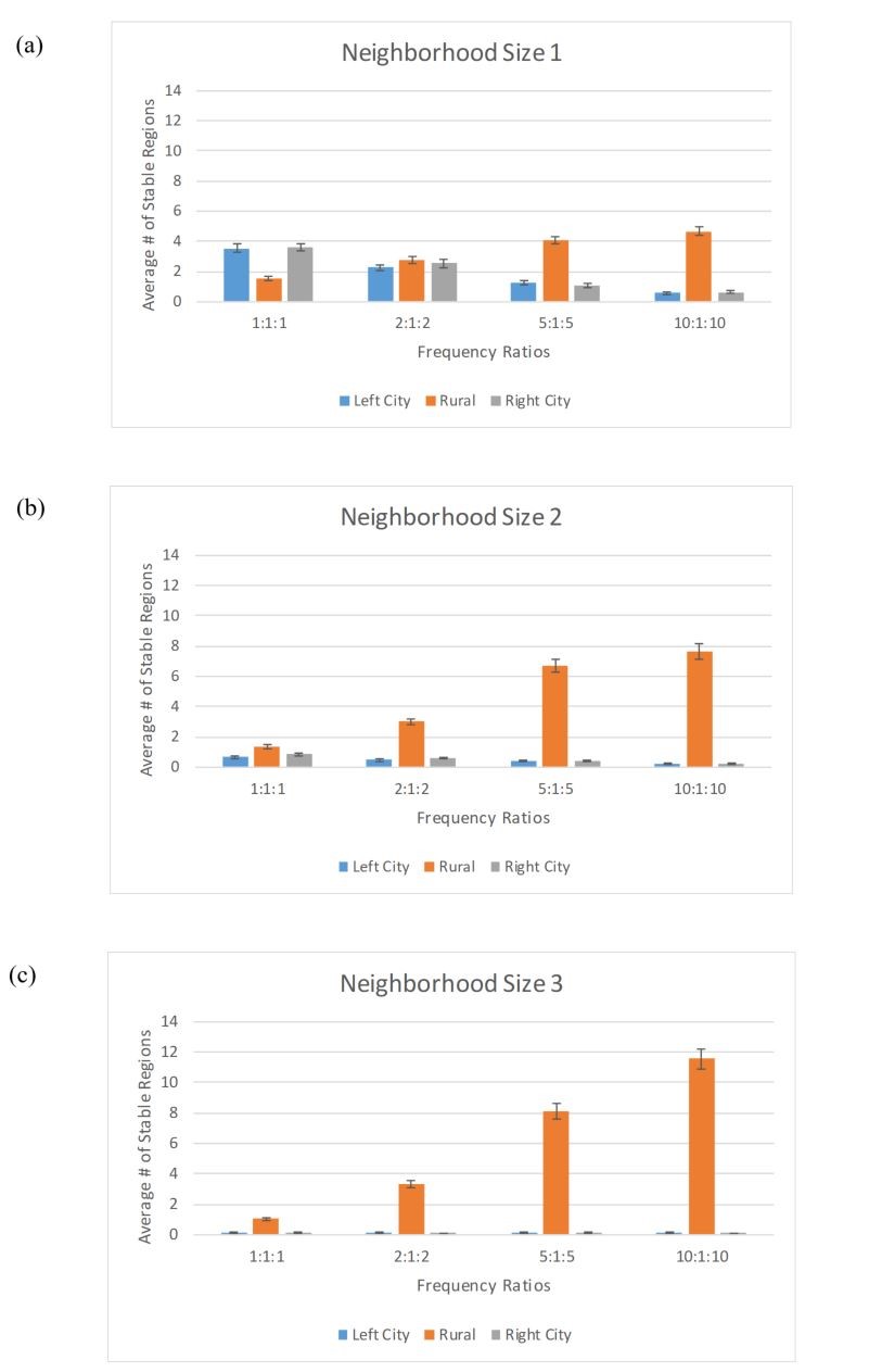
We next examine the effects on cultural diversity induced by increasing the frequency of interactions of the urban agents relative to that of the rural agents. Our primary findings are illustrated in Figure 7.
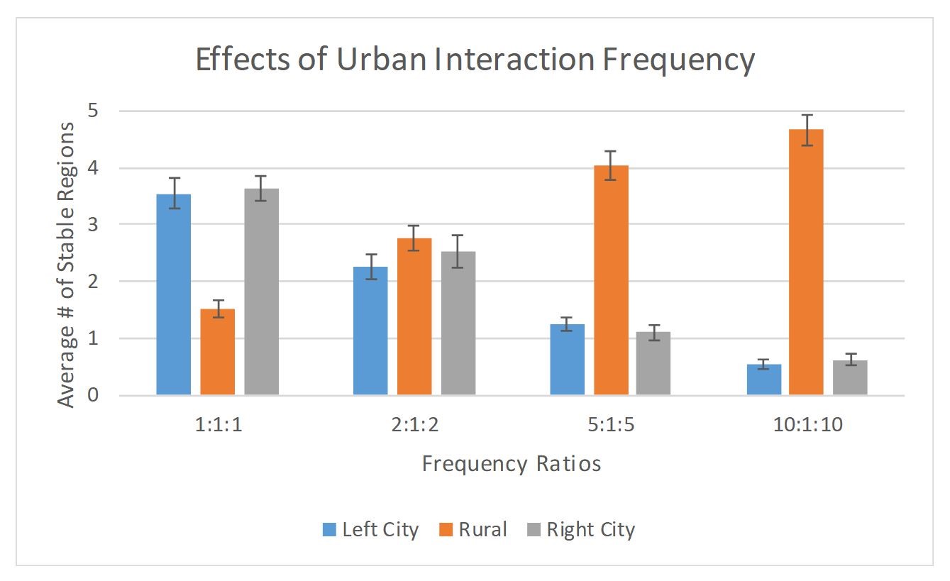
The simulation reveals an interesting, unanticipated phenomenon: As the frequency of agent interactions within the cities is increased, the urban areas \(C_L\) and \(C_R\) tend toward greater cultural homogeneity whereas the rural region R tends toward greater culturally diversity. Why this should be the case — i.e., why rural diversity should increase when urban agents interact more frequently — requires discussion. The origin of this phenomenon, we believe, is intimately related to the issue of timescales. Suppose the urban-agent interaction frequency is set much higher than that of the rural agents. City agents will thus update and evolve on a relatively rapid timescale compared to the evolution in the rural region. The city regions can thereby reach a sort of quasi-stasis — wherein they effectively have settled down to a quasi-absorbing state. Here, “quasi” signifies that the cities are not in true absorbing state since they will continue to evolve (since the rural region has not yet settled), though any subsequent changes in the cities will be relatively modest in scope. In this quasi-static state, the city regions effectively form a fairly steady, relatively homogeneous backdrop against which the rural region continues to evolve. In other words, from the perspective of the rural agents, the traits of the city agents appear almost frozen, and thus the probability of subsequent interaction and convergence of traits between urban and rural regions will be small, ultimately leading to more diversity within the rural regions.
As a test of this hypothesis, we model the following extreme scenario: Consider a 30x10 rural region bordered by two 30x1 strips of urban agents, wherein we assume the traits of these urban agents on the edges are all identical and fixed (i.e., cannot evolve). This 30x12 lattice is depicted in Figure 8.
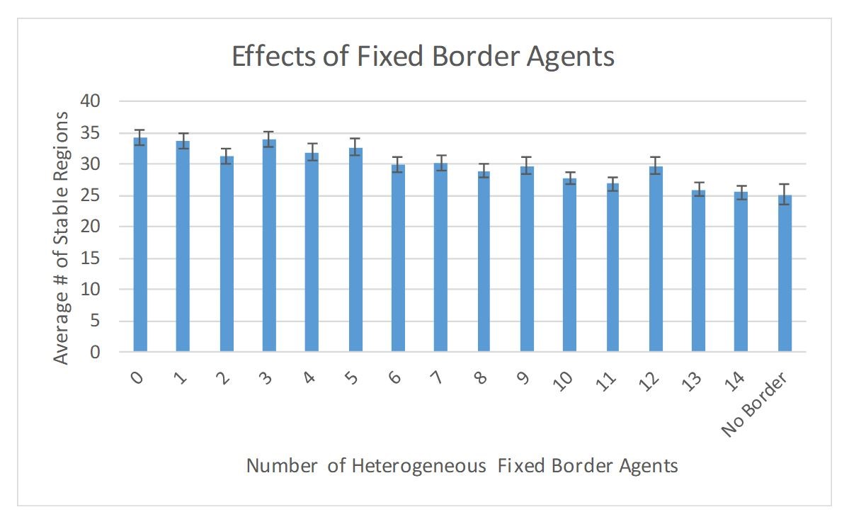
Here, the two strips of city agents play the role of a frozen boundary for the rural region. Numerical simulations show, in general, that surrounding a lattice with a fixed, completely homogeneous boundary promotes diversity within the lattice: Averaging over 100 trials, the mean number of stable regions in the rural area is 34±1 under this scenario. In contrast, if the boundary condition is relaxed somewhat so that not all of the (fixed) urban border agents have identical traits, or if we remove the fixed urban boundary strips altogether, leaving just a 30x10 rural grid, then the number of stable regions drops, demonstrating that indeed a fixed homogeneous boundary on a grid of agents boosts overall diversity. This observation, illustrated in Figure 9, demonstrates that the dynamical role of boundary conditions in these lattice models is crucial. Probing a bit more deeply, the emergence of this effect can be traced back in part to the question of whether or not the agents in the rural regions have had an opportunity to successfully interact with other agents prior to the simulation reaching stability. Our simulations show that, on average, a lattice with a fixed, completely homogeneous boundary (i.e., 30 identical, fixed, urban agents on each side) settles with 20±1 agents never having interacted, whereas a lattice whose border is a mixture of 16 identical and 14 heterogeneous urban boundary agents (all fixed) settles with 14.5±1 agents having had no interactions. These agents which haven’t participated in the interactions are important for cultural diversity because they typically stand alone as single-agent culturally diverse regions. This dovetails nicely with an earlier finding of Klemm et al. (2003a) who showed that lower-frequency cultural perturbations in ACM-like models tend to push a network of agents towards homogeneity while higher-frequencies perturbations prevent the system from ever settling. Here, we can think of the fixed heterogeneous border agents as a source of persistent yet relatively infrequent ‘perturbations’ on the rural agents.
Returning now to our original 30x30 urban-rural lattice model, effectively what appears to be happening is that the frequently interacting urban agents rapidly (quasi)-equilibrate, forming a quasi-frozen homogeneous boundary for the still-evolving rural region, thereby increasing the number of stable regions in R. This, in essence, is what we believe to be the underlying behavior responsible for the phenomenon seen in Figure 7.
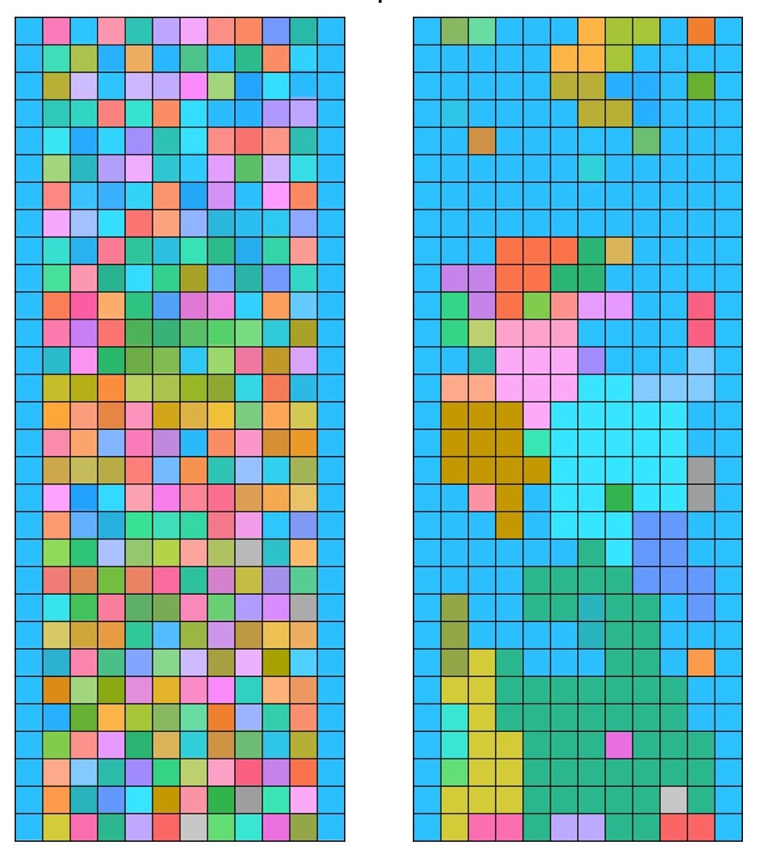
Lastly, we remark upon one additional interesting albeit rare occurrence associated with an increase in urban interaction frequency. In the vast majority of simulation runs, a single dominant culture emerges which permeates most of the lattice (both city and rural regions), save for a few small pockets of stable cultural states; Figure 3 depicts a representative example. However, if the urban-agent interaction frequency is high, a new phenomenon can occur, namely, the emergence of more than one dominant culture. An example is illustrated in Figure 10. It must be reiterated that this is a rarely occurring phenomenon. In such cases, what appears to be happening is that, owing to high-frequency urban interactions, there is rapid communication occurring separately in each of the two cities, \(C_L\) and \(C_R\) but insufficient communication between the two cities across \(R\) for synchronization of cultures to occur, the result being the emergence of more than one dominant culture. This split-cities effect is more likely to occur the higher the \(C_L:R:C_R\) ratios are. However, this phenomenon remains rare — even at a very high 10:1:10 frequency ratio, this effect occurred in only about 2% of trials.
Interplay between interaction range and frequency effects
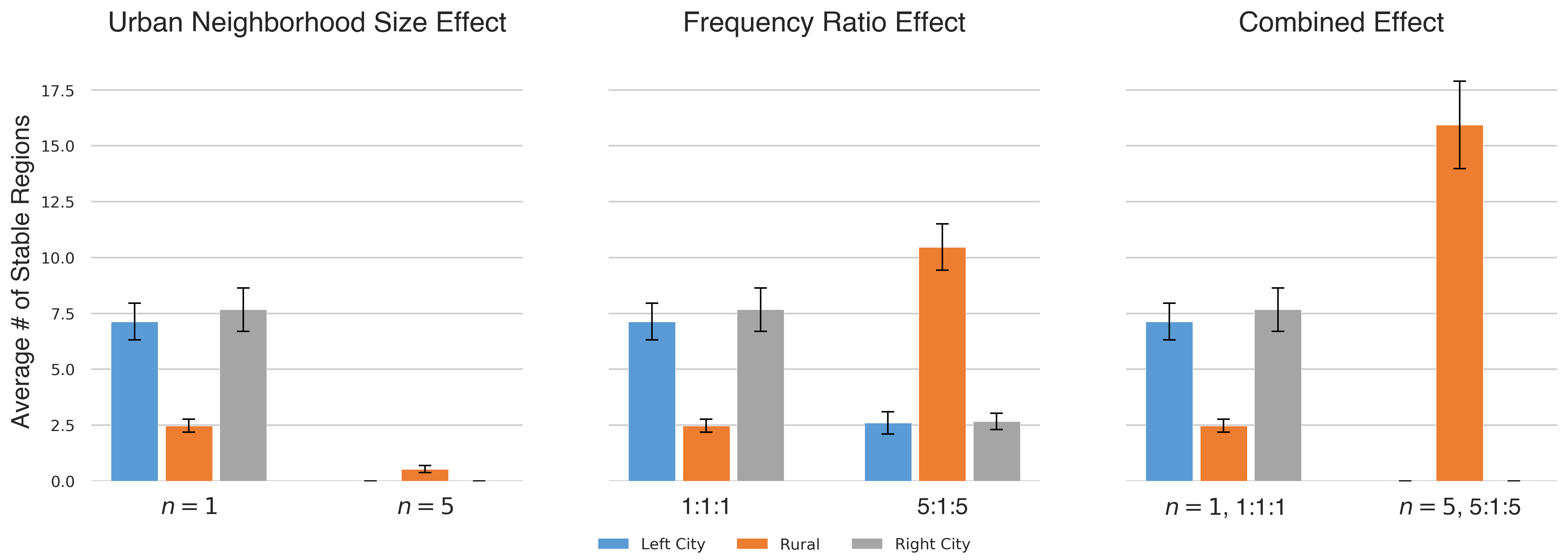
Thus far, we have seen (Figures 4 and 7) that (i) increased urban interaction range is associated with increased homogeneity in both the city \(C_L\), \(C_R\) areas and the rural \(R\) and (ii) increased urban interaction frequency produces increased homogeneity in the cities but decreased homogeneity in\(R\). Of particular note is that the responses of the rural region to increases in interaction range and in interaction frequency are in opposite directions. It is therefore of interest to consider the two competing influences in tandem. The results are intriguing. Our main findings are encapsulated in Figure 11, which shows the effects of interaction frequency for three different interaction ranges.
These simulations reveal that simultaneously increasing both urban interaction range and urban interaction frequency produces a marked increase in rural diversity. Indeed, comparing this to Figures 4 and 7 (which studied these two competing influences in isolation from one another), we observe here that the interplay between interaction range and frequency does not lead to some sort of balance or compromise in terms of their combined effect on rural diversity, but rather produces an unexpected amplification in rural diversity. This is a surprising effect, and not one that lends itself to a simple explanation. We point out that the fact that such a phenomenon is even possible — i.e., that two opposing influences, when combined, lead to an amplified response in one direction — can be appreciated by recalling that our underlying mathematical model represents a complex, nonlinear dynamical system, and as such there is no inherent reason why competing influences must average out. That said, we can conjecture as to what is happening here. Recall that higher urban frequency, considered in isolation, causes the urban agents to evolve and settle down towards a quasi-frozen state on a relatively fast timescale compared to rural agents. On the other hand, increasing urban interaction range, by itself, tends to produce greater urban homogeneity. So perhaps these two influences conspire to produce semi-frozen city regions which are more homogeneous than they would be otherwise. The rural region would therefore continue to slowly evolve against this semi-fixed backdrop of highly homogeneous city boundaries. This would, in accordance with the boundary arguments illustrated in Figure 8 and Figure 9, lead in turn to increased rural diversity compared to the case where the city boundaries are more heterogeneous.
While we previously noted that increasing urban interaction range alone led to more interactions in the rural region (Figure 5), pairing increased urban interaction range with high urban interaction frequency gives rise to the opposite effect. We observe in Figure 12 that as the urban interaction range increases from \(n=1\) to \(n=2\) and from \(n=2\) to \(n=3\), the average number of interactions in the rural region decrease by 24% and 16% respectively. We suspect that this decrease in rural agent interactions without the homogenizing effects of extended interaction ranges is a key contributor to the behavior we observe in Figure 11. We emphasize, however, that the explanatory scenario suggested here concerning the origin of the phenomenon illustrated in Figure 11 remains speculative and is not fully understood at the present time.
Related issues: Boundary effects and parameter choices
The results presented in the previous sections on the effects of interaction range and frequency on the heterogeneity of urban and rural regions relied on simulated lattices containing 900 agents, each of which had \(F=5\) features with \(q=15\) possible traits. Accordingly, several key questions need to be addressed: First, how important a role do boundary effects play in these results — i.e., as we go to larger system sizes in which the boundaries effects are diminished, do the previously observed trends concerning rural-urban development persist, or were they merely finite-size effects? Second, our initial choice of \(F=5\) and \(q=15\) was motivated by Axelrod’s work suggesting this was an interesting parameter regime to explore. However, from the work of Castellano et al. (2000) we know this choice lies on the “order” side of a non-equilibrium phase transition in the Axelrod model, which means that as the system size increases the system moves increasingly towards homogeneity. Thus we ask what happens if, as we increase system size, we simultaneously also move closer to the phase transition, for example, by increasing the number of traits \(q\)? A third question that we address in this section relates to the vector nature of the model itself. In our model each agent state was represented as a five-dimensional vector (\(F=5\)). Do our observations regarding rural-urban heterogeneity depend on the vector nature of the agent states, or can similar effects be seen in simpler scalar models? In what follows we briefly address each of these questions.
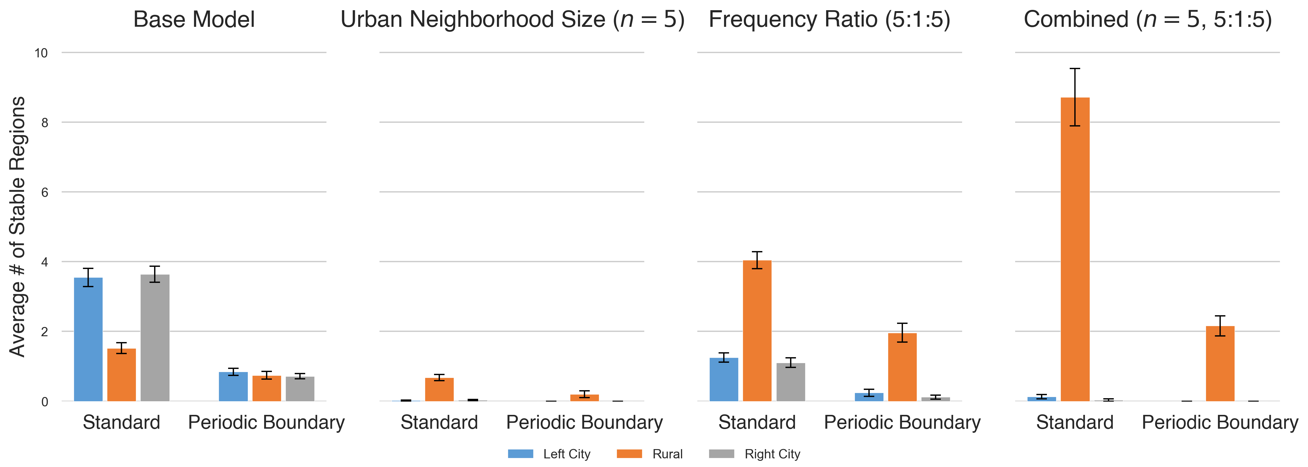
We first take up the issue of boundary effects. We test this in two ways. First, we look at the model’s behavior under periodic boundary conditions, wrapping the grid into a torus, with the two cities thereby connected. Second, we keep the original (non-periodic) boundary conditions intact but instead look at progressively larger grid sizes, going from 900 agents to 3,600 agents to 14,400 agents. As noted previously, in all cases we might anticipate that the absolute size of the observed heterogeneity will decrease, but the primary question of interest remains: Do the previously observed trends concerning rural-urban heterogeneity persist in terms of relative (rather than absolute) sizes? The short answer is yes. Although diminishing the impact of boundaries (via periodic boundary conditions and/or increasing lattice size) results in fewer stable cultural regions overall, we find that the interaction range effect, the interaction frequency effect, and combined effect qualitatively remain (though the combined effect is noticeably reduced). Figure 13 illustrates the case for periodic boundary conditions.
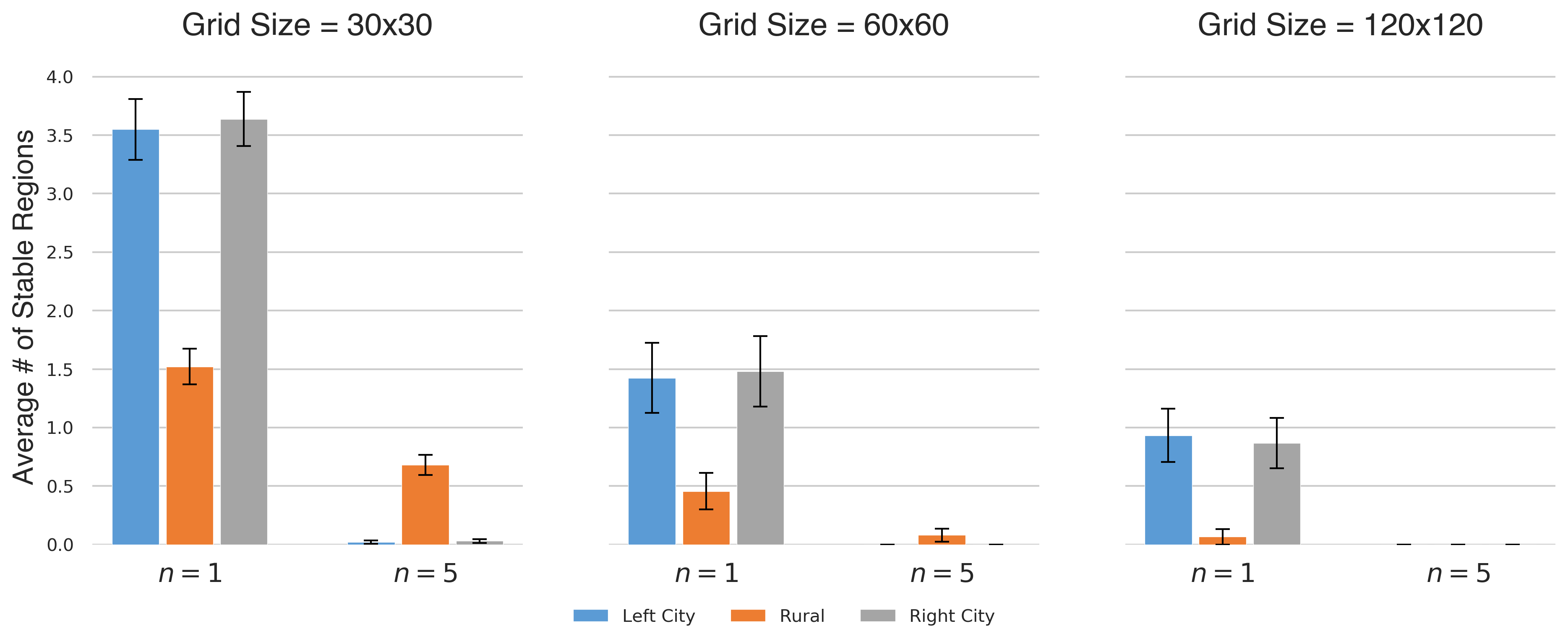
We next test the effects of the boundary by extending the size of the grid, such that the boundary agents become a smaller fraction of all agents. It is known that increasing the grid size results in fewer stable regions in the base model (Axelrod 1997). Figure 14 illustrates the effect of urban neighborhood size on heterogeneity, for different lattice sizes. We find that, as expected, the absolute level of heterogeneity in both urban and rural regions decreases for larger lattices (approaching zero for large enough lattices), but, just as before, we observe that the relative impact of increased neighborhood size in promoting homogeneity is more pronounced in the urban regions.
Next, we consider the effects of increasing interaction frequency on urban and rural heterogeneity for different lattice sizes (Figure 15). Although absolute heterogeneity levels decrease with lattice size, we again observe that higher interaction frequency in urban regions promotes heterogeneity in the rural region.
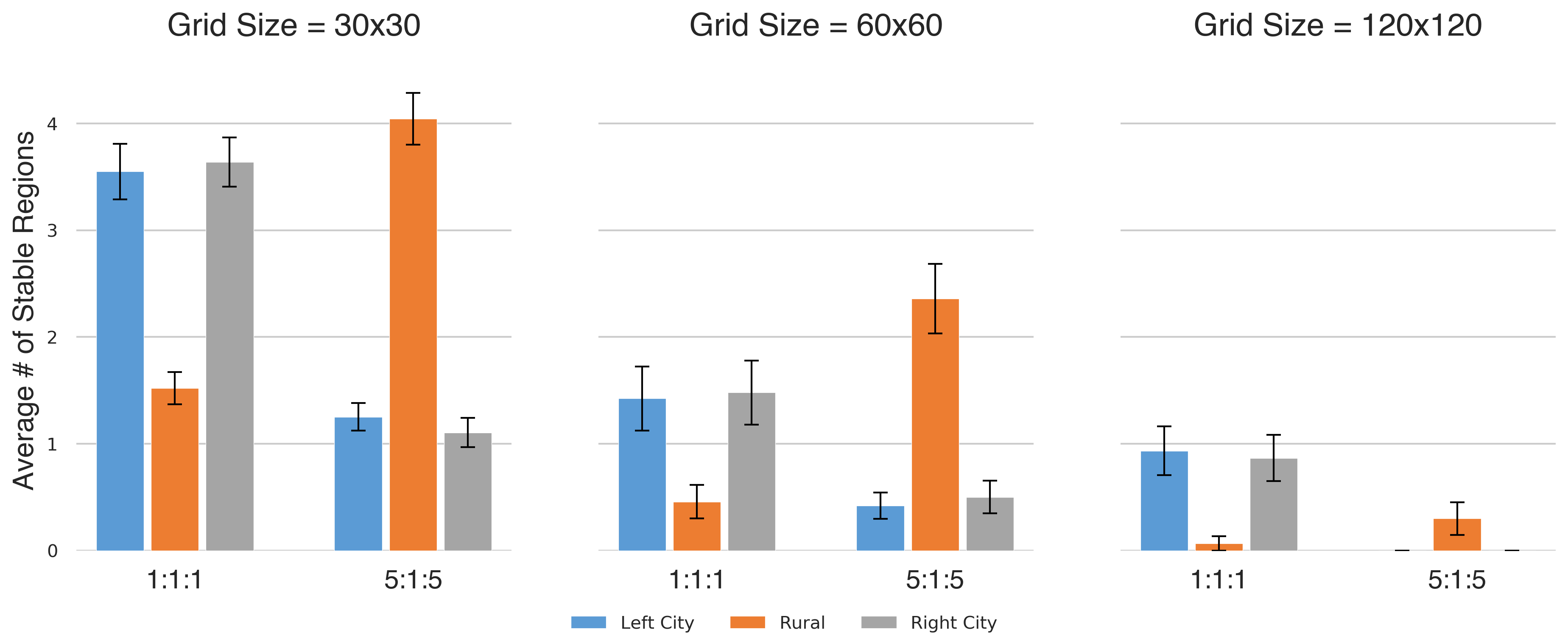
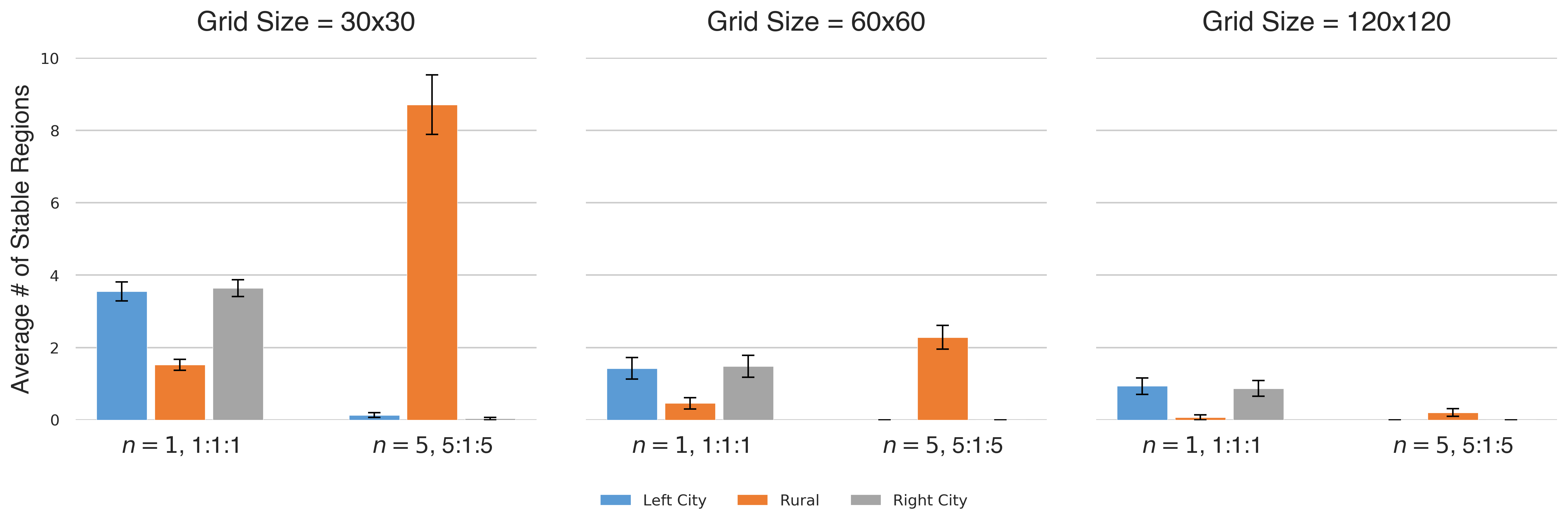
Figure 16 depicts the combined effects of simultaneously increasing neighborhood size and interaction frequency, for various lattice sizes. Comparison with Figure 14 and Figure 15 shows that, for small to moderate lattice sizes, the two effects combine to enhance the overall level of heterogeneity in the rural region, but this mutual reinforcement does not occur for larger lattice sizes.
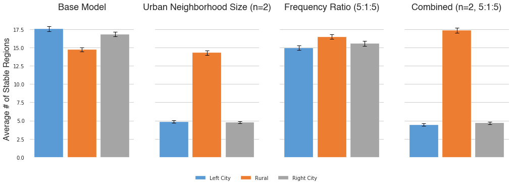
Next, we note although the number of stable regions naturally decreases with lattice side for a fixed number of features (\(F=5\)) and traits (\(q=15\)), we can compensate for this tendency by increasing the value of \(q\) (thereby bringing us closer to the phase transition described in Castellano et al. 2000). When doing so, we choose a value of \(q\) that does not surpass the phase transition, beyond which each agent in the model tends to make up its own distinct cultural region. On a lattice of length 120, we increase \(q\) to 20 and find the expected increase in the number of average stable regions, illustrated in Figure 17. Note that under these circumstances we find that all key aspects of our original findings persist on larger grid sizes, namely (i) as the urban interaction range is increased, the average numbers of cultural regions in both the urban and the rural areas are found to significantly decrease, (ii) as the urban interaction frequency is increased the average number of cultural regions decrease in the urban areas but, interestingly, increase in the rural area, and (iii) increasing both the urban interaction range and the urban interaction frequency together results in a significant increase in the number of cultural regions in the rural area.
Lastly, in order investigate whether our findings depend inherently on the vector nature of our models, or whether similar effects arise in scalar models, we conducted simulations based on a scalar model of cultural dissemination developed by Deffuant et al. (2000), wherein each agent’s culture is modeled as a single continuous scalar quantity between 0 and 1 rather than as an (\(F=5\) dimensional) vector. In the scalar model of Deffuant et al., agents interact if their cultures are within a threshold distance, and successful interactions result in the agents’ cultures becoming closer in value. We deviate from the precise lattice model described in Deffuant et al. (2000) in two ways: only the active agent’s culture changes after a successful interaction, and our simulation stops after all agents that are able to interact with their neighbors are within a set threshold of each other. Our findings are shown in Figure 18. In short, we do not find that this sort of highly simplified scalar model to be capable of reproducing the trends found in the richer vector model.
Concluding Remarks
Understanding the origin and nature of cultural disparities between urban and rural areas of society is an intriguing, highly relevant issue today. It is also a question of great complexity and debate. Indeed, disagreements on even the basic definitions of ‘urban’ and ‘rural’ have long presented challenges for researchers. Dewey (1960) surveys introductory sociology textbooks and a breadth related books and articles for definitions of urbanism (as distinguished from ruralism) and finds a wide range of criteria with no clear consensus. The United Nation’s World Urbanization Prospects report (2019) likewise outlines a number of distinct characterizations of urbanism across countries, including varying conditions on population, predominance of agricultural economic activity, and region characteristics such as the presence of street lighting and waste management. Definitions may vary even within a country — across government departments in the United Kingdom, for instance, there are over 30 distinct official definitions of rural (Scott 2007). Moreover, many sociologists are rejecting the notion of a rigid rural-urban dichotomy that is often presented by government agencies in favor of a continuum-based framework (McGranahan et al. 2014; Scott et al. 2007; Scala et al. 2017).
In this work, we have attempted to provide some partial insights into certain aspects of these issues, albeit not through an exhaustive examination of the full panoply of potential drivers of disparities between urban and rural regions (e.g., migration, work environments, economic opportunities, political affiliation, etc.). Nor is our intent to offer panoptic sociological definitions and explanations. Rather, we have focused on two simple yet fundamentally relevant factors in the cultural evolution of a social network — the frequency of one’s interactions with neighbors and the number of neighbors with whom to interact — and have asked how each of these factors affects cultural dissemination in different regions, and have examined the interplay between these two factors.
Our main findings offer some answers, highlight a few surprises, and raise a number of new, yet-to-be resolved questions. In particular, we have shown via our agent-based model that owing to the mutual interactions between urban and rural regions during the cultural dissemination process, the presence of a higher number of neighbors within urban regions tends to promote cultural homogeneity in both urban regions as well as rural regions. However, the higher frequency of interactions in urban regions, while also promoting more homogeneity within the urban regions, produces an unanticipated reduction in cultural homogeneity within rural regions (via some intriguing temporal and spatial interaction effects). Moreover, when considered in tandem, the larger neighborhood sizes and more frequent interactions within urban regions tend to combine in a manner that unexpectedly amplifies (in a manner which is still not fully understood) the level of heterogeneity within a rural region.
While the homogenizing effects of our urban assumptions may be counterintuitive given the common conception that heterogeneity is a key characteristic of urbanism (Dewey 1960), we emphasize that these findings speak only to the purely intrinsic effects of neighborhood size and interaction frequency on the behavior of a cultural network (independent of all other conflating factors), and that this work is not an attempt to explain all real-world underlying causes of cultural disparities between rural and urban regions. Nonetheless, refining and limiting the scope of our inquiry in this manner allows for substantive headway to be made, and we hope that this avenue of research might provide fodder for current social theories and discussions on the nature of urban-rural disparities.
Model Documentation
The model has been built in Python. The code to replicate our model is stored on the CoMSES Computational Model Library under the following url: https://www.comses.net/codebases/a2b1a1ed-a327-4ecc-9ee4-781aebe1db91/releases/1.0.0/.Acknowledgements
This work was supported in part with funding through a Keck Foundation Summer Research Fellowship, a Seaver Fellowship, and a Bekavac Summer Research Fellowship.References
ANDRES, L., & Looker, E. D. (2001). Rurality and Capital: Educational Expectations and Attainments of Rural, Urban/Rural and Metropolitan Youth. Canadian Journal of Higher Education, 31(2), 1-45.
AXELROD, R. (1997). The dissemination of culture: A model with local convergence and global polarization. Journal of Conflict Resolution, 41(2), 203-226. [doi:10.1177/0022002797041002001]
CAI, N., Diao, C., & Khan, M. J. (2017). A novel clustering method based on quasi-consensus motions of dynamical multiagent systems. Complexity, 2017. [doi:10.1155/2017/4978613]
CASTELLANO, C., Marsili, M., & Vespignani, A. (2000). Nonequilibrium phase transition in a model for social influence. Physical Review Letters, 85(16), 3536. [doi:10.1103/physrevlett.85.3536]
CENTOLA, D., Gonzalez-Avella, J. C., Eguiluz, V. M., & San Miguel, M. (2007). Homophily, cultural drift, and the co-evolution of cultural groups. Journal of Conflict Resolution, 51(6), 905-929. [doi:10.1177/0022002707307632]
DEFFUANT, G., Neau, D., Amblard, F., & Weisbuch, G. (2000). Mixing beliefs among interacting agents. Advances in Complex Systems, 3(01n04), 87-98. [doi:10.1142/s0219525900000078]
DELREAL, J. A., & Clement, S. (2017). Rural divide. The Washington Post.
DEWEY, R. (1960). The rural-urban continuum: Real but relatively unimportant. American Journal of Sociology, 66(1), 60-66. [doi:10.1086/222824]
GONZÁLEZ-AVELLA, J. C., Cosenza, M. G., Klemm, K., Eguíluz, V. M., & San Miguel, M. (2007). Information feedback and mass media effects in cultural dynamics. Journal of Artificial Societies and Social Simulation, 10(3), 9: https://www.jasss.org/10/3/9.html.
GREIG, J. M. (2002). The end of geography? Globalization, communications, and culture in the international system. Journal of Conflict Resolution, 46(2), 225-243. [doi:10.1177/0022002702046002003]
KATZ, J. (2016). ‘Duck Dynasty’vs.‘Modern Family’: 50 Maps of the US Cultural Divide. The New York Times.
KLEMM, K., Eguíluz, V. M., Toral, R., & San Miguel, M. (2003a). Global culture: A noise-induced transition in finite systems. Physical Review E, 67(4), 045101. [doi:10.1103/physreve.67.045101]
KLEMM, K., Eguíluz, V. M., Toral, R., & San Miguel, M. (2003b). Nonequilibrium transitions in complex networks: A model of social interaction. Physical Review E, 67(2), 026120. [doi:10.1103/physreve.67.026120]
KRON, J. (2012). Red state, blue city: How the urban-rural divide is splitting America. The Atlantic, 30.
LYONS, L. (2003). Communities of Faith. News Gallup Poll Tuesday Briefing. Feb. 11: https://news.gallup.com/poll/7756/communities-faith.aspx.
MCGRANAHAN, G., & Satterthwaite, D. (2014). Urbanisation Concepts and Trends. IIED Working Paper: https://pubs.iied.org/pdfs/10709IIED.pdf.
RODRÍGUEZ, A. H., & Moreno, Y. (2010). Effects of mass media action on the Axelrod model with social influence. Physical Review E, 82(1), 016111.
SCALA, D. J., & Johnson, K. M. (2017). Political polarization along the rural-urban continuum? The geography of the presidential vote, 2000–2016. The ANNALS of the American Academy of Political and Social Science, 672(1), 162-184. [doi:10.1177/0002716217712696]
SCOTT, A., Gilbert, A., & Gelan, A. (2007). The Urban-rural divide: Myth or reality?. SERG Policy Brief. Aberdeen: Macaulay Institute.
SHIBANAI, Y., Yasuno, S., & Ishiguro, I. (2001). Effects of global information feedback on diversity: Extensions to Axelrod's adaptive culture model. Journal of Conflict Resolution, 45(1), 80-96. [doi:10.1177/0022002701045001004]
SAN Miguel, M., Eguiluz, V. M., Toral, R., & Klemm, K. (2005). Binary and multivariate stochastic models of consensus formation. Computing in Science & Engineering, 7(6), 67-73. [doi:10.1109/mcse.2005.114]
UNITED Nations, Department of Economic and Social Affairs, Population Division (2019). World Urbanization Prospects: The 2018 Revision (ST/ESA/SER.A/420). New York: United Nations.
WILCOX, S., Castro, C., King, A. C., Housemann, R., & Brownson, R. C. (2000). Determinants of leisure time physical activity in rural compared with urban older and ethnically diverse women in the United States. Journal of Epidemiology & Community Health, 54(9), 667-672. [doi:10.1136/jech.54.9.667]
XIE, D., Liu, Q., Lv, L., & Li, S. (2014). Necessary and sufficient condition for the group consensus of multi-agent systems. Applied Mathematics and Computation, 243, 870-878. [doi:10.1016/j.amc.2014.06.069]