The Role of Reinforcement Learning in the Emergence of Conventions: Simulation Experiments with the Repeated Volunteer’s Dilemma

,
and
Utrecht University, Netherlands
Journal of Artificial
Societies and Social Simulation 25 (1) 7![]()
<https://www.jasss.org/25/1/7.html>
DOI: 10.18564/jasss.4771
Received: 10-May-2021 Accepted: 28-Dec-2021 Published: 31-Jan-2022
Abstract
We use reinforcement learning models to investigate the role of cognitive mechanisms in the emergence of conventions in the repeated volunteer’s dilemma (VOD). The VOD is a multi-person, binary choice collective goods game in which the contribution of only one individual is necessary and sufficient to produce a benefit for the entire group. Behavioral experiments show that in the symmetric VOD, where all group members have the same costs of volunteering, a turn-taking convention emerges, whereas in the asymmetric VOD, where one “strong” group member has lower costs of volunteering, a solitary-volunteering convention emerges with the strong member volunteering most of the time. We compare three different classes of reinforcement learning models in their ability to replicate these empirical findings. Our results confirm that reinforcement learning models can provide a parsimonious account of how humans tacitly agree on one course of action when encountering each other repeatedly in the same interaction situation. We find that considering contextual clues (i.e., reward structures) for strategy design (i.e., sequences of actions) and strategy selection (i.e., favoring equal distribution of costs) facilitate coordination when optima are less salient. Furthermore, our models produce better fits with the empirical data when agents act myopically (favoring current over expected future rewards) and the rewards for adhering to conventions are not delayed.Introduction
Conventions solve coordination problems that occur in everyday life, from how to greet each other in the street, to what to wear at a black-tie event, to what citation style to use in a paper. Conventions can be deliberately introduced (e.g., citation styles), but they can also emerge tacitly, as a consequence of individual actions and interactions (Centola & Baronchelli 2015; Lewis 1969; Sugden 1986; Young 1993). Results from experiments with economic games show that incentives matter for the conventions that can emerge in repeated social interactions (Diekmann & Przepiorka 2016). That is, individuals engage more in certain behaviors the less costly it is to do so. However, how cognitive processes, such as learning, interact with structural properties of the situation in the emergence of conventions is less well understood (Przepiorka et al. 2021; Simpson & Willer 2015).
Here, we use agent-based simulations to investigate the role of learning in the emergence of conventions in the repeated, three-person volunteer’s dilemma game (VOD). The VOD is a binary choice, n-person collective goods game in which a single player’s volunteering action is necessary and sufficient to produce the collective good for the entire group (Diekmann 1985). For example, a couple awaken by their crying baby face a VOD with regard to who should get up and calm the baby. A group of friends wanting to go out in town on Friday night face a VOD with regard to who should drive and abstain from drinking alcohol. The members of a work team that embarks on a new project face a VOD with regard to who should take the lead. In all these situations, every individual prefers to volunteer if no one else does, but prefers having someone else do it even more.
An important distinction can be made between symmetric and asymmetric VODs (Diekmann 1993). In a symmetric VOD, all players have the same costs and benefits from volunteering. In an asymmetric VOD, at least two players have different costs and/or benefits from volunteering. Previous research shows that a turn-taking convention, in which each player incurs the cost of volunteering sequentially, can emerge in the symmetric VOD. In an asymmetric VOD, in which one player has lower costs of volunteering, a solitary-volunteering convention emerges by which the individual with the lowest cost volunteers most of the time (Diekmann & Przepiorka 2016; Przepiorka et al. 2021).
Following the concept of “low (rationality) game theory” (Roth & Erev 1995 p. 207), we conduct simulation experiments with adaptive learning (rather than “hyperrational”) agents to explain experimental data. That is, we compare three classes of reinforcement learning models to study how the process of learning contributes to the emergence of the turn-taking convention and the solitary-volunteering convention in the repeated symmetric and asymmetric VOD, respectively. Through simulation experiments and validation with human experimental data, we gain insights into potential mechanisms that can explain how individuals learn to conform to the expectations of others. Specifically, we address two research questions (RQs): (1) How well do different classes of reinforcement learning models fit the human experimental data? (2) Which model properties affect the fit with the experimental data?
By addressing these questions, we expect to learn whether reinforcement learning models can provide a cognitive mechanism that can explain the emergence of conventions (RQ1) and what parameter settings are needed to simulate human behavior (RQ2). Reinforcement learning models are widely used in cognitive modeling and cognitive architecture research. Having such an existing mechanism as a candidate explanation for a wider range of problems, is preferred over introducing new mechanisms to explain behavior (cf. Newell 1990). Our work provides such a critical test.
The remainder of the paper is structured as follows. We first review literature that has used cognitive modeling to explain the emergence of conventions in humans and outline the contribution our paper makes to this literature by focusing on the repeated, three-person VOD. We then recap the principles of reinforcement learning models and introduce the three model classes that we focus on in this study. The next three sections outline the simulation procedures, list and describe the parameters we systematically vary in our simulation experiments, and describe our approach to the analysis of the data produced in our simulation experiments. The results section presents our findings, and the final section discusses our findings in the light of previous research and points out future research directions.
Previous Literature
Reinforcement learning as cognitive mechanism of convention emergence
Cognitive science has shown a growing interest in the role of cognitive mechanisms in the emergence of social behavior. A review article by Hawkins et al. (2019) points out that a potentially fruitful area for cognitive science research is ‘the real computational problems faced by agents trying to learn and act in the world’ (p. 164). Spike et al. (2017) identify three important factors to address this gap: (1) the availability of feedback and a learning signal, (2) having a mechanism to cope with ambiguity, and (3) a mechanism for forgetting. Cognitive modeling studies of conventions have so far focused mainly on the mechanism of memory and forgetting in two-player social interaction games (e.g., Collins et al. 2016; Gonzalez et al. 2015; Juvina et al. 2015; Roth & Erev 1995; Stevens et al. 2016). These models showed that learning to play the game requires fine-tuning of associated cognitive mechanisms (e.g., parameters for learning, forgetting), and that learned behavior can, within limits, transfer to other game settings (Collins et al. 2016).
Here we focus on a factor that has been under-explored, namely the role of feedback and a learning signal. More specifically, we investigate whether social decision-making observed in a computerized lab experiment with the three-person VOD can be explained based on reinforcement learning models of cognitive decision-making (RQ1), and what characteristics such reinforcement learning models should have (RQ2).
The basic task of a reinforcement learning agent is to learn how to act in specific settings, so as to maximize a numeric reward (Sutton & Barto 2018). Reinforcement learning models have been used in two ways to study the emergence of conventions. The first family of reinforcement learning models takes an explanatory approach and are designed to study how empirical data comes about. Roth & Erev (1995), for example, used adaptive learning agents to study data collected in experiments on bargaining and market games. In a very abbreviated form, agents select actions based on probabilities for these actions, while probabilities are derived from the averaged rewards obtained for these actions in the past. Roth & Erev (1995) showed that the dominant experimental behavior of perfect equilibrium play is in principle explainable by reinforcement learning. However, agents required more than 10,000 interactions before patterns stabilized. Other studies demonstrated how conventions can emerge from the interaction between reinforcement learning and other cognitive mechanisms, such as declarative memory (Juvina et al. 2015). However, these models also required the introduction of separate, novel cognitive mechanisms (e.g., ‘trust’) to provide a good fit with empirical data (see also Collins et al. 2016). Introduction of new mechanisms to fit results from a new context (e.g., the VOD) is at odds with the general objective of cognitive modeling to have a fixed cognitive architecture that can explain performance in a variety of scenarios (Newell 1990).
The second family (e.g., Helbing et al. 2005; Izquierdo et al. 2007,2008; Macy & Flache 2002; Sun et al. 2017; Zschache 2016, 2017) uses reinforcement learning to identify what the objectively best policy is to handle scenarios. Such models allow one to identify whether humans apply the optimal strategies for solving a learning problem, or to compare whether (boundedly) rational agents opt for strategies predicted by game-theoretical considerations. Sun et al. (2017), for example, studied tipping points in the reward settings of a Hawk-Dove game variant beyond which conventions can be expected to emerge. Izquierdo et al. (2007,2008) found that settings with high learning and aspiration rates move quickly from transient regimes of convention emergence to asymptotic regimes of stable conventions. Zschache (2016, 2017) showed that an instance of melioration learning, namely Q-Learning (Watkins & Dayan 1992), produces stable patterns of game-theoretical predictions and that these patterns emerge much quicker (~factor 100) than in the Roth-Erev model. In contrast to explanatory models (e.g., Roth & Erev 1995), this family of models takes an exploratory approach to study the general conditions that contribute to the emergence of conventions.
In our paper, we follow an explanatory approach (family 1), while avoiding the addition of a separate mechanism (e.g., trust), to investigate whether (RQ1), and under what conditions (RQ2), reinforcement learning alone can explain the emergence of conventions in the repeated three-person VOD. We explore three different classes of reinforcement learning models to investigate how generalizable results are across models and parameter settings. We evaluate our models against a previously reported empirical dataset collected by Diekmann & Przepiorka (2016), described briefly at the end of this section.
The use of economic games to study convention emergence
In behavioral and experimental social science, the emergence of conventions is often observed in laboratory experiments with economic games in which the same group of participants interact with each other repeatedly (Camerer 2003). The structure of the game that emulates the interaction situation in one round can vary in terms of payoffs of individual group members and how these payoffs are reached contingent on these group members’ actions (i.e., strategies). The bulk of the experimental research uses symmetric games, i.e., games in which the roles of players are interchangeable because all players face the same payoffs from their actions. More recently, however, it has been recognized that asymmetric games may better capture the individual heterogeneity that occurs in real-life settings (Hauser et al. 2019; Kube et al. 2015; Otten et al. 2020; Przepiorka & Diekmann 2013, 2018; van Dijk & Wilke 1995). In asymmetric games, players differ in their payoffs and their roles are therefore not interchangeable.
Moreover, the experimental literature on the emergence of cooperation in humans has mostly used linear collective goods games, in which each unit a player contributes increases the collective good by the same amount (Andreoni 1995; Chaudhuri 2011; Fischbacher et al. 2011). With a few exceptions, only more recently, threshold and step-level collective good games are used in experimental research (Dijkstra & Bakker 2017; Milinski et al. 2008; Rapoport & Suleiman 1993; van de Kragt et al. 1983).
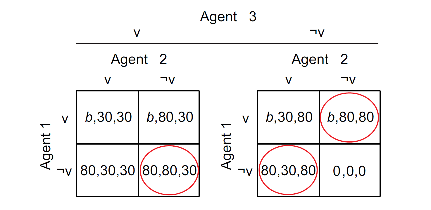
The VOD falls into the realm of step-level collective good games, and a distinction can be made between the symmetric and an asymmetric VOD. Figure 1 presents a three-person version of the VOD in normal form. In the symmetric VOD, all three players have the same costs of and benefits from volunteering (\(b = 30\)), while in the asymmetric VOD, one “strong” player has lower costs of volunteering, which manifests itself in higher net benefits for that player (\(80 > b > 30\); e.g., \(b = 70\)). The game has three Pareto optimal, pure-strategy Nash equilibria (circled in red in Figure 1), in which only one player volunteers while the other two players abstain from volunteering. Furthermore, it has one mixed-strategy Nash equilibrium in which all players volunteer with a certain probability (Diekmann 1985, 1993). In the asymmetric VOD, rational players can tacitly coordinate on the pure strategy Nash equilibrium in which only the strong player volunteers, even if the game is played only once (Diekmann 1993; Harsanyi & Selten 1988). In the symmetric VOD, tacit coordination on one of the pure-strategy equilibria is more difficult. If, however, the symmetric game is repeated over an indeterminate number of rounds, turn-taking among all three players becomes a salient, Pareto optimal Nash equilibrium (Lau & Mui 2012). Although solitary volunteering by the strong player remains a salient Nash equilibrium in the asymmetric game if the game is repeated, it leads to an inequitable distribution of payoffs as the strong player obtains a lower payoff than the other two in every round (Diekmann & Przepiorka 2016).
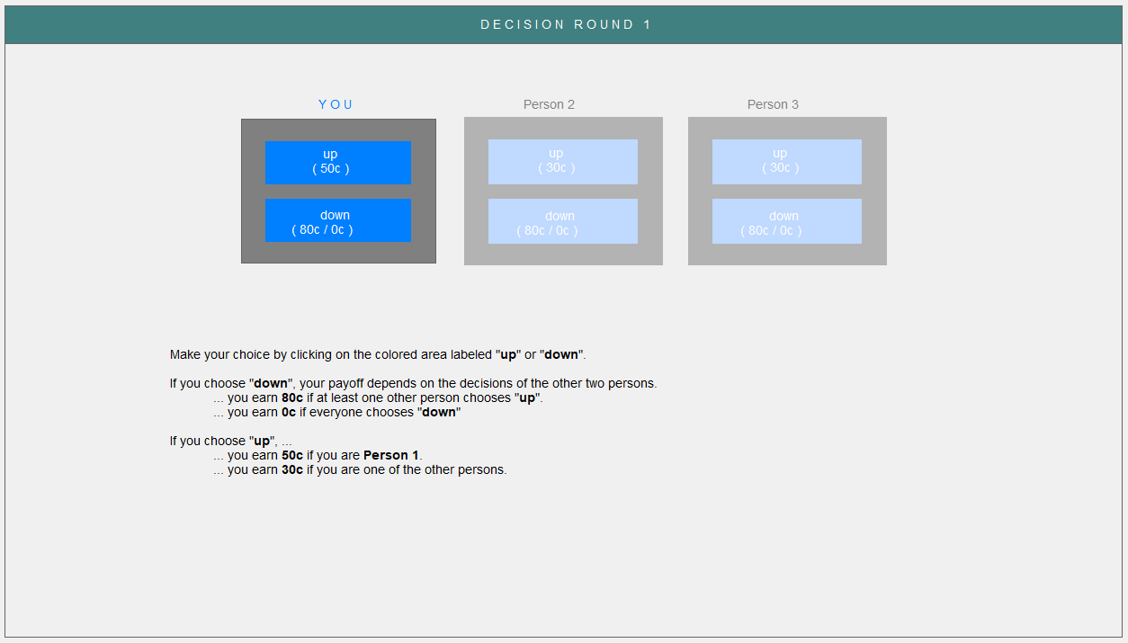
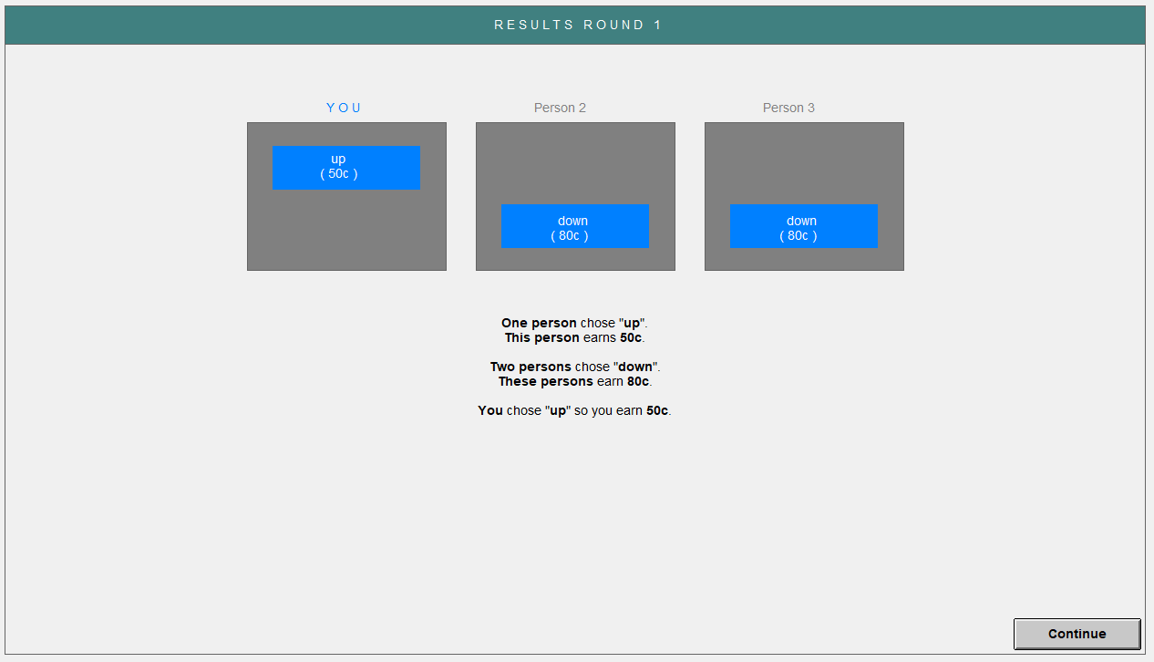
In their experiment, Diekmann & Przepiorka (2016) matched participants randomly in groups of three and assigned them to either the symmetric VOD or an asymmetric VOD condition. In all experimental conditions, participants interacted with the same group members in the VOD for 48 to 56 rounds. In each round, they faced the same VOD, made their decisions individually and independently from each other and were provided with full information feedback on the decisions each group member took and these group members’ corresponding payoffs (see Figures 8 and 9 in the Appendix). The payoffs each participant gained in each round were summed and converted into money that participants received at the end of the experiment. Diekmann & Przepiorka (2016) found that in the symmetric VOD, a turn-taking convention emerges, whereas in an asymmetric VOD, a solitary-volunteering convention emerges. While in turn-taking each group member volunteers and incurs a cost sequentially, in solitary-volunteering the group member with the lowest cost of volunteering, volunteers most of the time. This finding has been replicated in several follow-up experiments (Przepiorka et al. 2021, 2022).
Our paper contributes to the research on step-level collective good games by investigating how differences in emergent conventions are reflected in cognitive models to better understand how conventions come about (Guala & Mittone 2010; Tummolini et al. 2013; Young 1993). In order to draw meaningful conclusions about how humans learn to coordinate in social settings, and thus how conventions emerge, our research uses reinforcement learning models to explain the empirical observations made by Diekmann & Przepiorka (2016) in their behavioral lab experiment.
Methods
Reinforcement learning models
Generally speaking, reinforcement learning agents learn what actions to pick based on the rewards that their actions result in. Reinforcement learning has a solid theoretical basis in behavioral psychology (Herrnstein & Vaughan 1980) and neuroscience (e.g., Schultz et al. 1997), generates empirically validated predictions (e.g., Herrnstein et al. 1993; Mazur 1981; Tunney & Shanks 2002; Vaughan Jr 1981), and finds applications in multiple cognitive architectures (e.g., Anderson 2007; Laird 2012). From the available realizations of reinforcement learning models, we consider Q-Learning (Watkins & Dayan 1992) as the prime candidate for our study. That is because, on the one hand, Q-Learning has been proven informative and efficient in previous game-theoretic contexts of convention emergence (Zschache 2017). On the other hand, Q-learning models are parsimonious in that they do not require additional mechanisms nor a full representation of their environment, but only a defined state they are in at a certain time (\(s_{t}\)) and the available actions in that state (\(a_{t}\)). Given that there is no need for a detailed model of the world, these Q-learning models are also referred to as model-free. Quality values (Q-values) for state-action pairs (\(Q(s_{t}; a_{t})\)) track how rewarding an action was at a given state, and form the basis of the decision making process. That is, the most rewarding action in a given state (\(max \; Q(s_{t}; a_{t})\)) is typically given priority. Moreover, Q-values are constantly updated based on the sum of their old values and anticipated new values (Sutton & Barto 2018):
| \[ Q(s_{t}; a_{t}) \leftarrow Q(s_{t}; a_{t}) + \alpha[r_{t+1} + \gamma max_{a} Q(s_{t+1}; a)-Q(s_{t}; a_{t})]\] | \[(1)\] |
New Q-values are composed of the actual reward \(r_{t+1}\) received after action \(a_{t}\) in state \(s_{t}\) and the maximum expected reward in a future state (\(s_{t+1}\)) from all available actions (\(max_{a} Q(s_{t+1}; a)\)). In our models, expectations depend on agents’ social preferences and are set to be the same for all agents at the beginning of a simulation run. Furthermore, setting expectations to high but achievable rewards ought to minimize the time of convention emergence (Izquierdo et al. 2007, 2008). Selfish agents, therefore, expect to receive the reward for the optimal individual action, while altruistic agents expect to receive the reward for the optimal collective action.
The impact of future rewards on Q-value updates is moderated by a discount factor and a learning rate. The discount factor (\(0 \leq \gamma \leq 1\)) parameterizes the importance of expected future Q-values relative to immediate rewards. Smaller \(\gamma\) values make the agent more ‘short-sighted’ and rely more heavily on immediate rewards (\(r_{t+1}\)), whereas larger \(\gamma\) values place more weight on long-term rewards (\(Q(s_{t}; a_{t})\)). The learning rate (\(0 < \alpha \leq 1\)) defines the extent of new experiences (both \(r_{t+1}\) and \(Q(s_{t+1}; a_{t})\)) overriding old information. Models with smaller \(\alpha\) values adjust their Q-values more slowly, and as a result, rely more heavily on experience than on most recent rewards.
Action selection typically considers a process to balance between exploitation of (currently) most rewarding actions (highest Q-value) and exploration of alternatives (lower Q-values that might also lead to success). A common approach for this is \(\epsilon\)-greedy, which defines a probability \(\epsilon\) for the selection of a random action, while the most rewarding action is selected with probability \(1-\epsilon\). This is especially useful in changing environments, so that low rewarding actions are still considered and may become more rewarding when conditions change. In our scenario, however, conditions do not change over time, so that there is no reason for agents to change strategies when there is one superior strategy. Furthermore, patterns in the experiment were mostly stable once they emerged, so that humans seem to stick to clearly best performing actions. To account for the stability of conditions and human behavior, we add noise to the calculated Q-values (\(Q_{noisy}\)) each time that an action is decided, rather than taking an \(\epsilon\)-greedy approach.
In our models, the noise is drawn from a continuous uniform distribution with parameter \(\eta\). Each time that a \(Q_{noisy}\)-value is calculated, a value within the range \([-\eta, \eta]\) is randomly drawn and multiplied with the original Q-value. The action that is associated with the highest \(Q_{noisy}\)-value is then selected for execution by the model. Mathematically, this can be expressed as:
| \[ \begin{gathered} max \; Q_{noisy}(s_{t+1}; a), \; with \\ \forall a: Q_{noisy}(s_{t}; a) \leftarrow Q(s_{t}; a) + [Q(s_{t}; a) \times \rho], \; and \\ \rho \sim U[-\eta, \eta] \end{gathered}\] | \[(2)\] |
Consequently, when a Q-value of one action is clearly superior, the corresponding action will be exploited. In cases where two or more actions have comparable Q-values, the noise factor regulates the frequency between exploration and exploitation. That is, the higher the setting for \(\eta\) the more explorative the model.
Model classes
Within the basic reinforcement learning framework outlined above, we define three model classes that differ in their assumptions. We call these model classes ClassicQ, SequenceX, and VolunteerX. This allows us to test how well the reinforcement learning models work in general, and to what degree they depend on additional model assumptions. All three models follow the concept of Markov chains (Gagniuc 2017). That is, they consist, first, of well-defined states and, second, of events that define the transition between these states (see Figure 2).
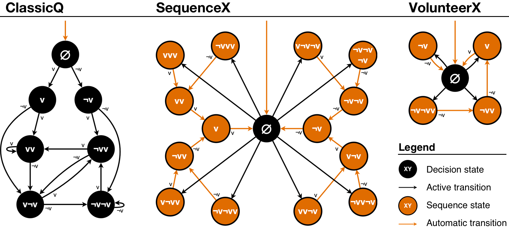
The ClassicQ model class uses a typical approach for Q-Learning. In the three-person VOD, actions can be to either volunteer or not volunteer: \(a \in \{v, \neg v\}\). States are defined by the actions an agent took in the previous two rounds: \(s \in \{vv, v\neg v, \neg vv, \neg v\neg v\}\). Available Q-values for ClassicQ are therefore: \(Q(vv; v)\), \(Q(vv; \neg v)\), \(Q(v\neg v; v)\), \(Q(v\neg v; \neg v)\), \(Q(\neg vv; v)\), \(Q(\neg vv; \neg v)\), \(Q(\neg v\neg v; v)\), \(Q(\neg v\neg v; \neg v)\). Furthermore, ClassicQ requires an initialization phase of two rounds (Figure 2, top three states). Here, every agent volunteers with a probability of 0.33 in each of the two rounds, as only one of the three agents is required to volunteer for the optimal outcome. All following actions are selected based on Q-values. Consider, for example, an agent that did not volunteer in the last two rounds (\(s_{t} = \neg v\neg v\); Figure 2, bottom right state of the ClassicQ model). Depending on the larger (noisy) Q-value (see Equation 2) for the currently available state actions pairs (\(Q(\neg v\neg v; v)\) and \(Q(\neg v\neg v; \neg v)\)), the agent decides to volunteer (Figure 2, active transition from state \(\neg v\neg v\) to state \(\neg vv\)) or to not volunteer (Figure 2, active transition from state \(\neg v\neg v\) back to state \(\neg v\neg v\)). As ClassicQ’s actions are influenced by two past states, we refer to this as a backward-looking perspective.
By contrast, the SequenceX and VolunteerX model classes follow a forward-looking perspective. That is, actions are defined by sequences of consecutive future actions (Figure 2, orange states), which are automatically and without reconsideration performed in the following rounds: \(a \in \{vvv, vv\neg v, v\neg vv, \dots\}\). Agents select a new action sequence whenever no actions are left to perform (\(s = \emptyset\)). Our models look forward at most 3 actions.
SequenceX defines action sequences for the next three actions, independent of what the preceding actions were. That is, the options are: \(Q(\emptyset; vvv)\), \(Q(\emptyset; vv\neg v)\), \(Q(\emptyset; v\neg vv)\), \(Q(\emptyset; v\neg v\neg v)\), \(Q(\emptyset; \neg vvv)\), \(Q(\emptyset; \neg vv\neg v)\), \(Q(\emptyset; \neg v\neg vv)\), \(Q(\emptyset; \neg v\neg v\neg v)\). Consider, for example, an agent that has no more actions left to perform (\(s_{t} = \emptyset\)). The agent selects an action sequence, depending on the largest (noisy) Q-value (see Equation 2) for all action sequences (e.g., \(v\neg vv\) – Figure 2, bottom left state), and performs the corresponding actions in the following three rounds (\(a_{t} = v\); \(a_{t+1} = \neg v\); \(a_{t+2} = v\)).
VolunteerX, in contrast, minimizes the length of action sequences by only defining when to volunteer. We used a strategy space from “immediately” to “in the third round”: \(Q(\emptyset; v)\), \(Q(\emptyset; \neg vv)\), \(Q(\emptyset; \neg v\neg vv)\). In addition, we included a strategy to not volunteer in the following round: \(Q(\emptyset; \neg v)\).
To summarize, all three model classes make decisions based on Q-values, which are shaped by experience, and which consider a sequence of up to three states and/or actions. However, the models differ in whether they are backward looking (ClassicQ: last two actions determine what Q-learning options are available) or forward-looking (SequenceX and VolunteerX consider all state-action pairs when deciding the next action). From a practical perspective, each time that ClassicQ needs to determine a next action, it can only choose between two Q-values out of all eight potential options (e.g., if the last two actions were \(v\) and \(\neg v\), then the only choice is between \(Q(v\neg v; v)\) and \(Q(v\neg v; \neg v)\)). SequenceX and VolunteerX, in contrast, consider all Q-values whenever a new action sequence is selected (eight options for SequenceX, and four for VolunteerX).
Conditions
We tested two different payoff conditions, which were identical to the “Symmetric” and “Asymmetric 2” conditions in the experiment by Diekmann & Przepiorka (2016) (also see Figure 1). In the Symmetric condition, all agents experience the same benefit if the collective good is produced (\(r_{1,2,3} = 80\)) and they incur the same costs when they volunteer to produce the collective good (\(K_{1,2,3} = 50\)). In the Asymmetric 2 condition (henceforth Asymmetric), all agents experience the same benefit when someone volunteers to produce the collective good (\(r_{1,2,3} = 80\)), however the cost for volunteering is lower for one agent (\(K_{1} = 10\)), compared to the other two agents (\(K_{2,3} = 50\)).
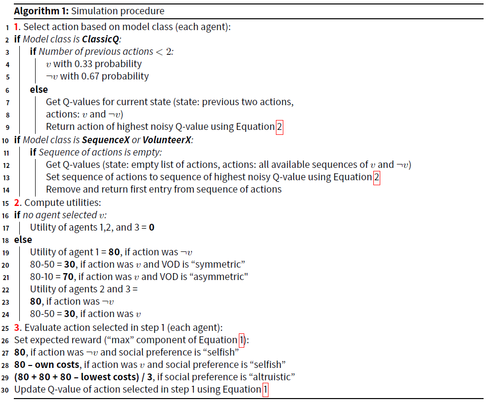
Simulation procedure
To test the behavior of our model classes, we simulated the experimental setup of Diekmann & Przepiorka (2016) with learning agents adopting the role of human participants. Each simulated game lasted 150 rounds2. A single round consisted of the following steps:
Parameter settings
For each model class, five parameters (see Table 1) were varied systematically:
- Discount rate (\(\gamma\)) describes the importance of expected future rewards relative to immediate rewards. As there is no consensus in the literature, we tested a wide range of values. This ranged from models that consider distant rewards equal to immediate rewards (\(\gamma = 1\)), to models that discount future rewards strongly (e.g., \(\gamma = 0.5\), rewards that are 1 step away are halved).
- Learning rate (\(\alpha\)) defines the extent of new experiences overriding old information. As there is no consensus in the literature, we tested a wide range of values. They ranged from models that relied relatively heavily on previous experience (\(\alpha\) close to 0.2) to models that rely more heavily on recent experience (\(\alpha\) close to 0.7).
- Initial Q-values (\(\iota\)) concern the initial value that each state-action pair gets assigned before running simulations. If the Q-value deviates a lot from the eventual learned value, the learning trajectory takes longer (as the new Q-value is impacted by \(\alpha\) and \(\gamma\)). Moreover, in such cases the model might get stuck in local optima earlier (i.e., if an initial action yields a very high reward relative to the expected value, then noise cannot overcome this selection). Therefore, we tried two values of the initial value: a payoff close to the theoretic optimum in the symmetric condition of (67.5) and one that is substantially lower (43.33).
- Exploration rate (\(\eta\)) defines the range of how much noise is randomly added to the Q-values before an action is selected (Equation 2). We distinguish between two scenarios: agents that are either more (\(\eta = 0.1\)) or less conservative (\(\eta = 0.2\)) in exploring new actions as a result of noise.
- Social preference (\(S\)) manipulates how the expected maximum reward (see Equation 1) is composed. For selfish agents, the expected reward (\(max_{a} Q(s_{t+1}; a)\)) corresponds to the highest possible individual reward. For altruistic agents, the expected reward corresponds to the highest possible collective reward.
| Variables | Possible value range | Values tested |
| Discount rate | \(0 \leq \gamma \leq 1\) | \(\gamma = \{0.50, 0.55, 0.60, 0.65, 0.70, 0.75, 0.80, 0.85, 0.90, 0.95, 1.00\}\) |
| Learning rate | \(0 < \alpha \leq 1\) | \(\alpha = \{0.50, 0.55, 0.60, 0.65, 0.70, 0.75, 0.80, 0.85, 0.90, 0.95, 1.00\}\) |
| Initial Q-values | \(\iota \geq 0\) | \(\iota\) = \(\{43.33, 67.5\}\) |
| Exploration rate | \(0 < \eta < 1\) | \(\eta\) = \(\{0.1, 0.2\}\) |
| Social preference | \(S \in \{selfish, altruistic\}\) | \(S\) = \(\{selfish, altruistic\}\) |
The final assumption in our model is that the above parameters and settings are related to the general “cognitive architecture” (Anderson 2007; Newell 1990) of the agents. In other words, when specific parameter values were set (e.g., \(\alpha = 0.4\), \(\gamma = 0.9\), \(\eta = 0.1\), \(\iota = 67.5\)), all three agents in the VOD assumed these parameter values. The only thing that might differ between them were the volunteering costs (\(K\)) in the asymmetric VOD. Although in practice different agents might differ in their cognitive architecture and in the way that they weigh different types of information (e.g., have different learning rates), keeping the values consistent across agents allowed us to systematically test how model fit changes in response to parameter changes (RQ2). This in turn helped us to understand what is more important for a good model fit: a change in model class (ClassicQ vs SequenceX vs VolunteerX) or a change in model parameters (e.g., when each model achieves an equally good fit with its “best” parameter set).
Data and Analysis
We had three model classes (ClassicQ, SequenceX, and VolunteerX), tested in two experimental conditions (symmetric and asymmetric VOD), for two types of reward integration (selfish or altruistic), with 484 (\(11 \times 11 \times 2 \times 2\)) parameter combination options (see Table 1). For each unique combination of these parameters, we ran 10 simulations. This resulted in a total of 58,080 (\(3 \times 2 \times 2 \times 484 \times 10\)) simulation runs. For each run, three agents interacted in 150 rounds of the VOD game.
To answer RQ1 (how well each model class fits the human experimental results), we first compute the mean Latent Norm Index (\(LNI\); Diekmann & Przepiorka 2016) for the 10 simulation runs per condition and model class. The \(LNI_{k,m}\) describes the proportion of behavioral pattern \(k\) that emerged in a group of size \(m\) in a given number of rounds. The behavioral patterns that are commonly found in experiments with the repeated three-player VOD are solitary-volunteering (\(k = 1\)), turn-taking between two players (\(k = 2\)), and turn-taking between all three players (\(k = 3\)) (see also Przepiorka et al. 2021). Since the empirical data we aim at reproducing are based on interactions between three participants, we use three agents in our simulation experiments (\(m = 3\)).
Consider, for example, the following sequence of actions in which positive numbers denote the index of a single volunteering player (i.e., player 1, 2 or 3) per round and 0 denotes rounds in which either no or more than one player volunteered: 1112310123. The game has a single sequence of player 1 volunteering three times in a row (1112310123). A game of 10 rounds therefore results in 30% solitary-volunteering (\(LNI_{1,3} = 30\%\)). It follows further that the same sequence maps to 0% turn-taking between two players (\(LNI_{2,3} = 0\%\)) and 70% turn-taking between all three players (1112310123; \(LNI_{3,3} = 70\%\)). Note that to avoid the detection of pseudo patterns, a pattern needs to be stable for at least \(m\) consecutive rounds to be counted towards the \(LNI\). For a detailed description of how the LNI is calculated, refer to Diekmann & Przepiorka (2016, p. 1318 f.).
To answer how well our models match the empirical data, we use root-mean-square errors (RMSE) between mean LNI of the simulated data and the LNI observed in the empirical data, with lower RMSE indicating a better model fit.
To answer RQ2 (which model properties affect model fit), we perform multiple linear regressions with RMSE as dependent variable and the model parameters as independent variables. This allows to understand the direction and size of the effect of each parameter on a model’s fit to the empirical data. We fit a total of six regression models: for each of our three model classes we fit one model to the data from the symmetric VOD condition and one from the asymmetric VOD condition. All parameters are centered at their means and only main effects are considered. We also fitted models with interaction effects. Since these models did not produce different insights (i.e., the main effects remained the same), we do not refer to them in the text. All regression model results are presented in the Appendix.
Results
RQ1: Model fit to empirical data
Figure 3 shows relative frequencies of the different conventions that emerged in the asymmetric VOD condition (left) and the symmetric VOD condition (right) in the empirical study of Diekmann & Przepiorka (2016) (gray bars) and our simulation experiments (colored bars) in terms of \(LNI\)s. The bars in the “Solitary volunteering”, “Turn taking 2” and “Turn taking 3” panels show average \(LNI_{1,3}\), \(LNI_{2,3}\) and \(LNI_{3,3}\), respectively. The different colored bars denote the results of the best fitting model instances of each model class (ClassicQ, SequenceX, and VolunteerX).
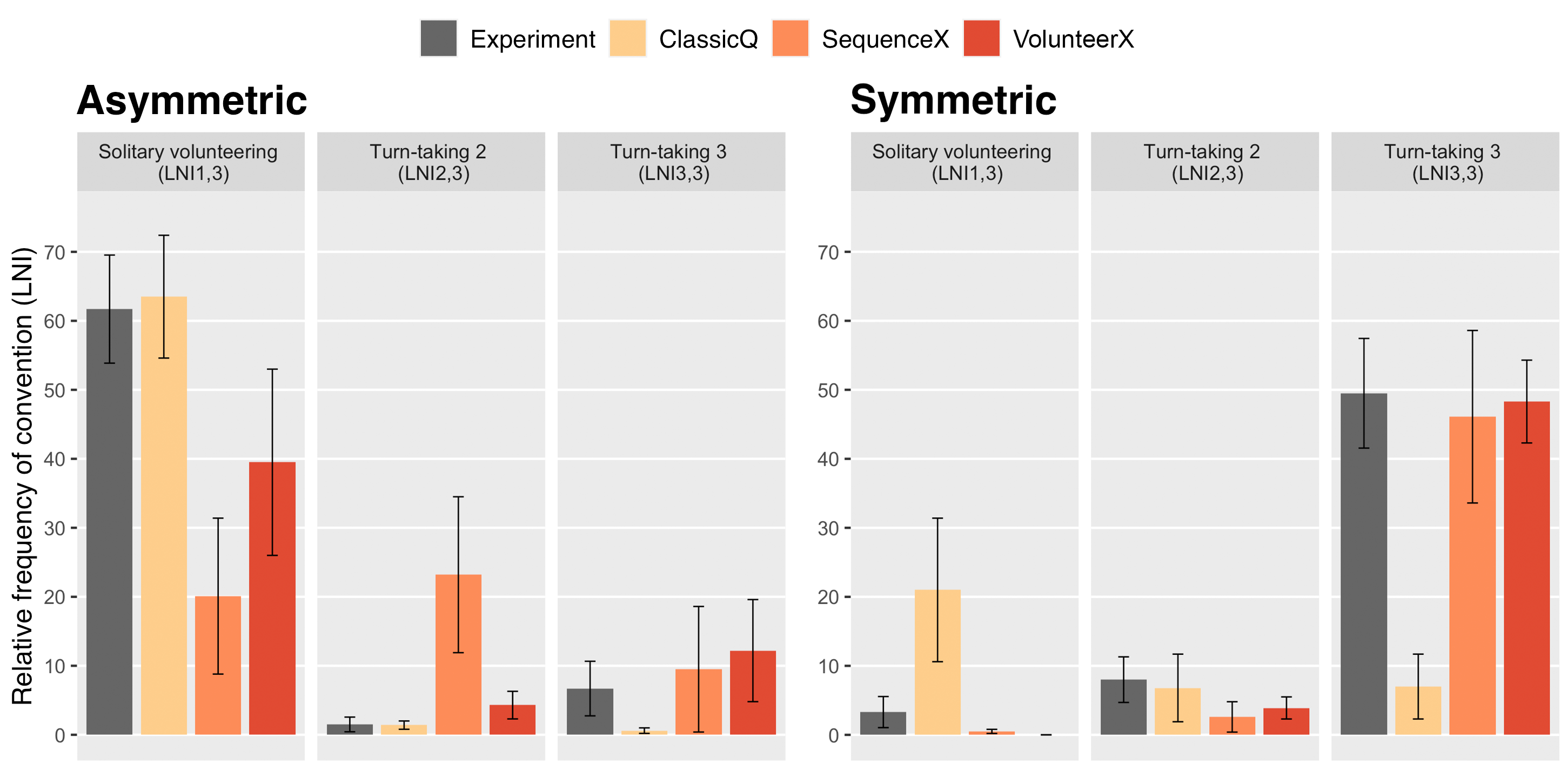
In the asymmetric cases, where one agent has lower costs from volunteering, the human data shows more frequent solitary volunteering. Of the three model classes, the ClassicQ model reproduces the dominant pattern of the empirical data (solitary volunteering) best. By contrast, in the symmetric case, where each agent has the same costs and benefits of volunteering, the human data shows frequent turn-taking between all three agents. ClassicQ is now the worst fitting model, as it hardly shows such turn-taking between three agents. SequenceX and VolunteerX show comparable results, where the percentage of trials with frequent turn-taking between three agents is comparable to the human data. As we will see in more detail below, variations in the relative frequency of patterns are a result of different stabilization times for single emerging patterns (ClassicQ in the asymmetric VOD, SequenceX and VolunteerX in the symmetric VOD) or multiple emerging patterns (ClassicQ in the symmetric VOD, SequenceX and VolunteerX in the asymmetric VOD).
To further study the properties of the model classes, Table 2 reports the best fitting (i.e., lowest mean RMSE) model instances (unique combination of the model class, reward integration, and parameter settings)3 per condition. The rows show mean RMSE per condition. The columns show the best fitting model instances per model class and condition (e.g., CQ.291 for ClassicQ and asymmetric VODs). Therefore, each model class has potentially three different model instances that produce a best fit. A single model instance of the SequenceX model class (SX.145), however, produced best fits in the asymmetric condition and in the combination of both conditions. Model instances that produce best fit per model class and condition are marked with a grey background. A \(*\) symbol denotes which of the three model classes provided the best overall fit across conditions.
| ClassicQ | SequenceX | VolunteerX | ||||||
|---|---|---|---|---|---|---|---|---|
| CQ.47 | CQ.291 | CQ.110 | SX.145 | SX.182 | VX.157 | VX.239 | VX.213 | |
| Asymmetric only | 4.18 | 3.87* | 35.68 | 25.02 | 37.7 | 15.59 | 13.47 | 33.08 |
| Symmetric only | 32.89 | 36 | 26.44 | 17.63 | 6.77 | 17.4 | 16.3 | 5.11* |
| Asym. and sym. | 20.07 | 24.01 | 32.24 | 19.57 | 26.29 | 16.51* | 18.11 | 23.87 |
| Note: The best fitting models are the models with the lowest RMSE. Within each column, the RMSE score is highlighted for the model that had the best score within that condition (e.g., combined, asymmetric and/or symmetric). Per row (combined, asymmetric, symmetric), the overall best fitting model is marked with a \(*\). | ||||||||
Consistent with Figure 3, a ClassicQ instance (CQ.291) produces the best fit of the three model classes in the asymmetric condition (RMSE = 3.87), while the instances producing best fits for SequenceX (SX.145 with RMSE = 25.02) and VolunteerX (CX239 with RMSE = 13.47) produce patterns less consistent with the empirical data. Further, we find good fits in the symmetric condition for SequenceX (SX.182 with RMSE = 6.77) and VolunteerX (VX.213 with RMSE = 5.11), while ClassicQ produces the worst fit of all best fitting models across both conditions (CQ.110 with RMSE = 26.44).
It is striking, however, that all of the models producing best fits in one condition produce comparably low fits in the other condition (e.g., CQ.291 with RMSE = 3.87 for asymmetric VODs and RMSE = 36.00 for symmetric VODs). Further, when considering the model instance producing the best fit in the combination of both conditions (VX.157 with RMSE = 16.51), two things become apparent. First, the model fit is significantly lower than the models producing best fits per condition (asymmetric: CQ.291 with RMSE = 3.87; symmetric: VX.213 with RMSE = 5.11). Second, the model fit per condition is also significantly lower than the models producing best fits per condition (RMSE = 15.59 for asymmetric VODs and RMSE = 17.40 for symmetric VODs). It follows that there is no single model able to closely replicate the human data in both conditions.
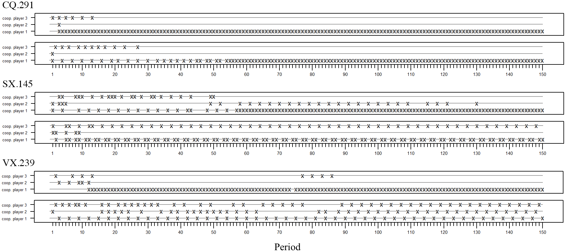
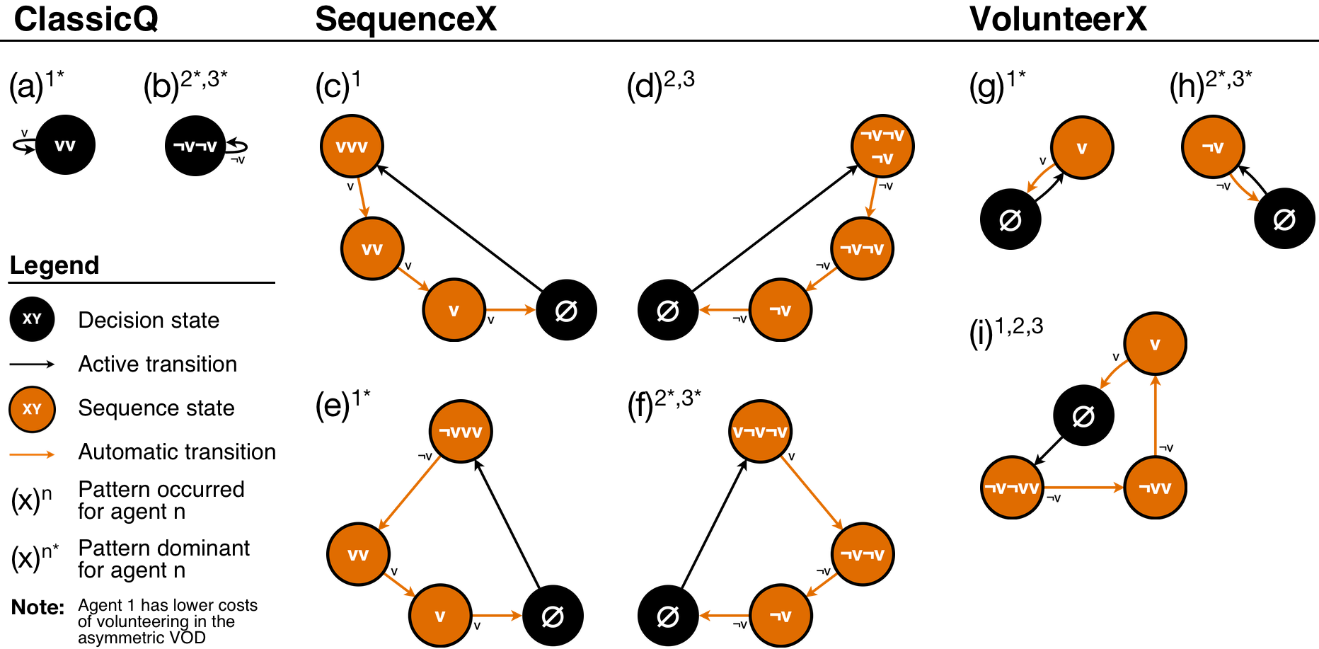
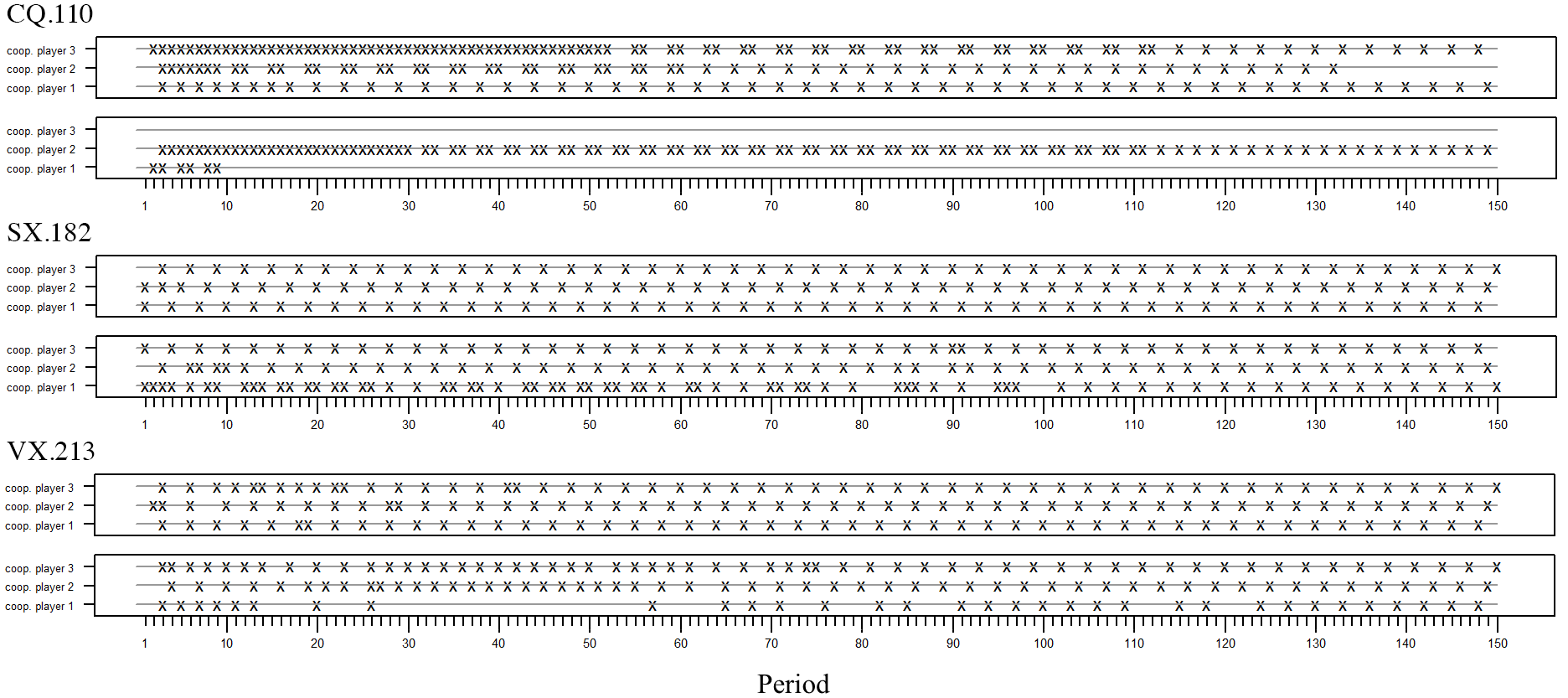
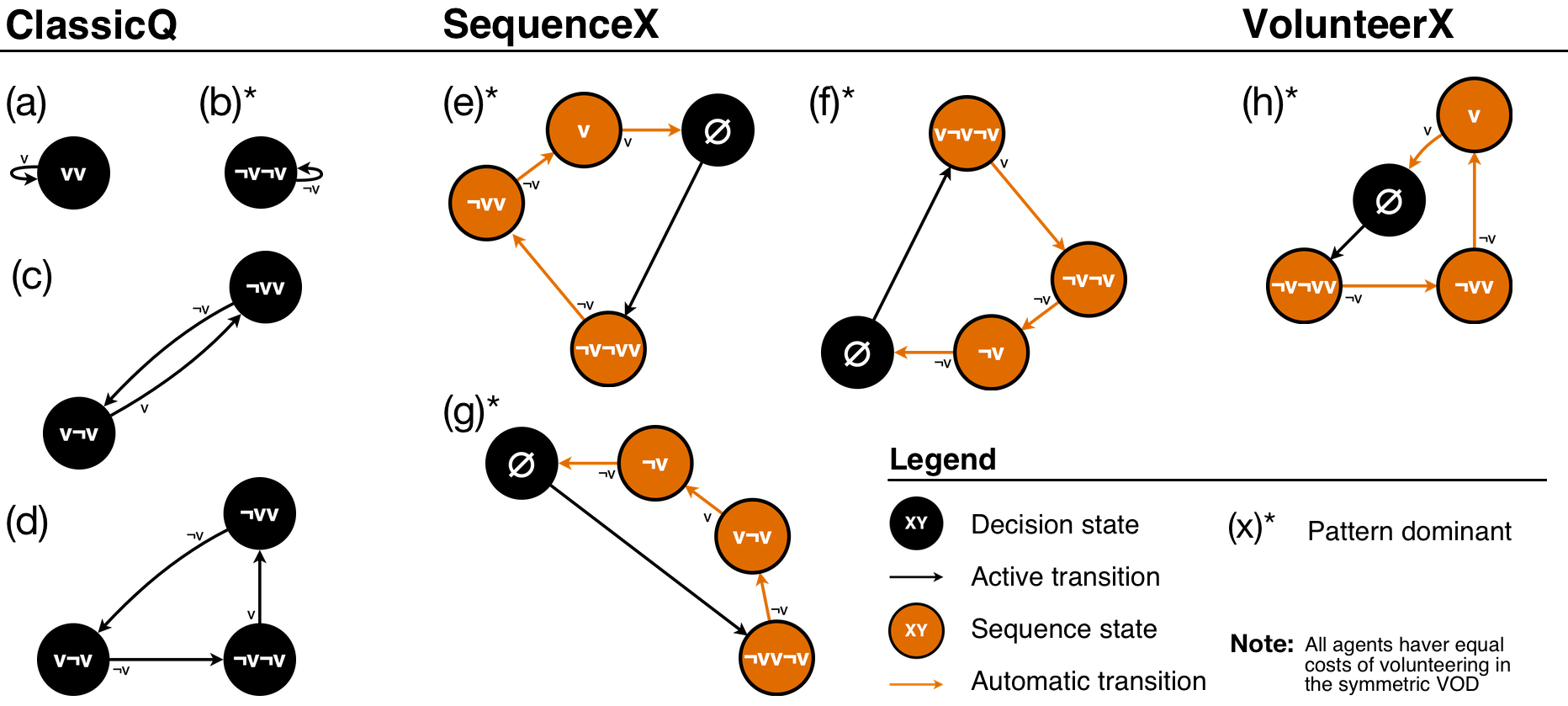
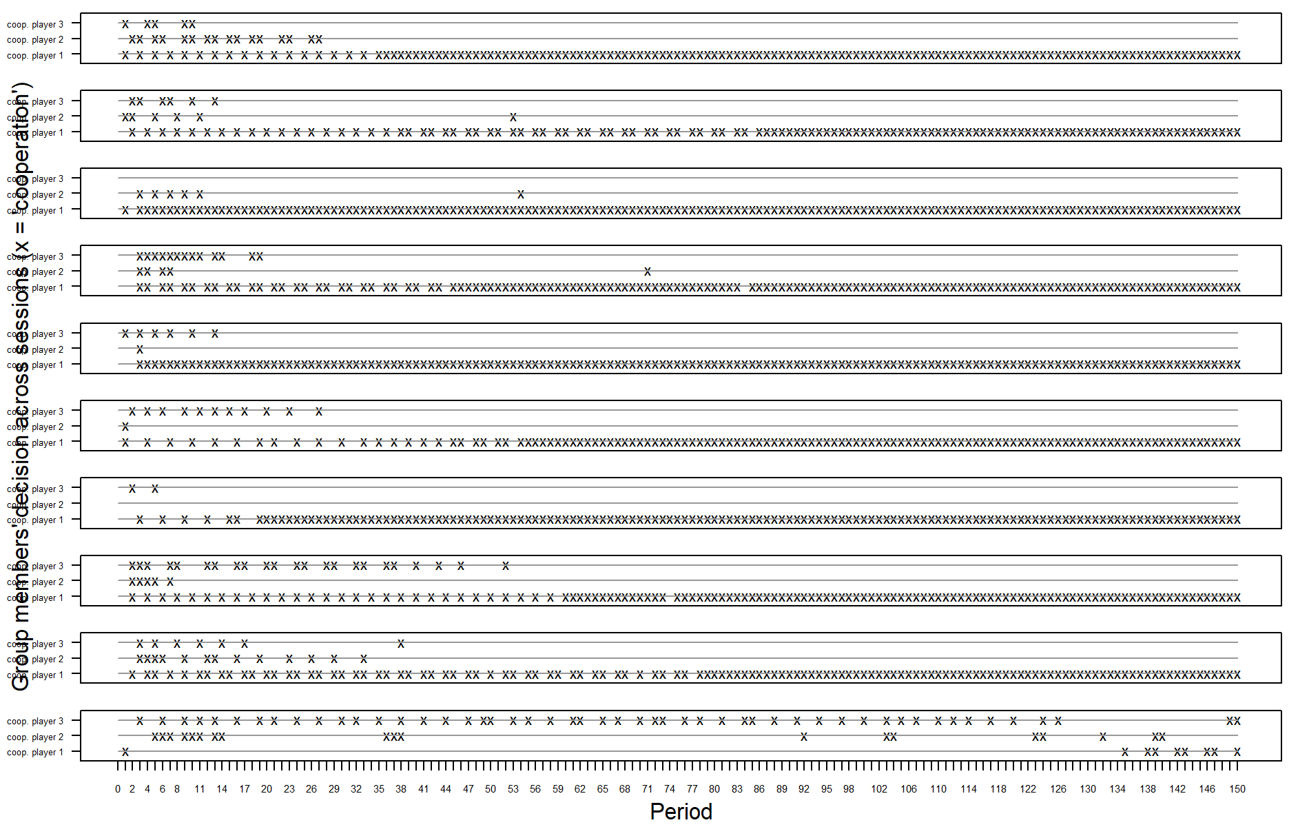
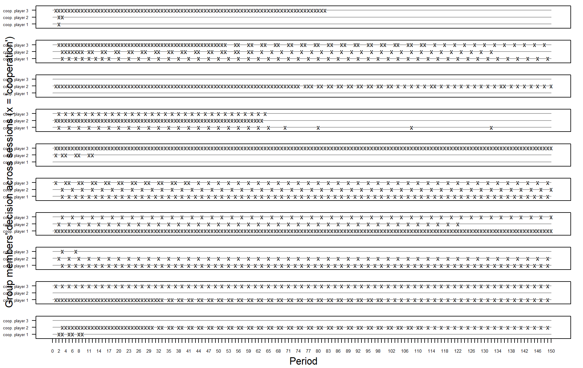
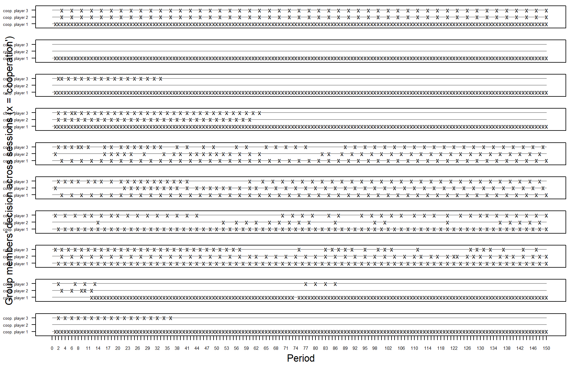
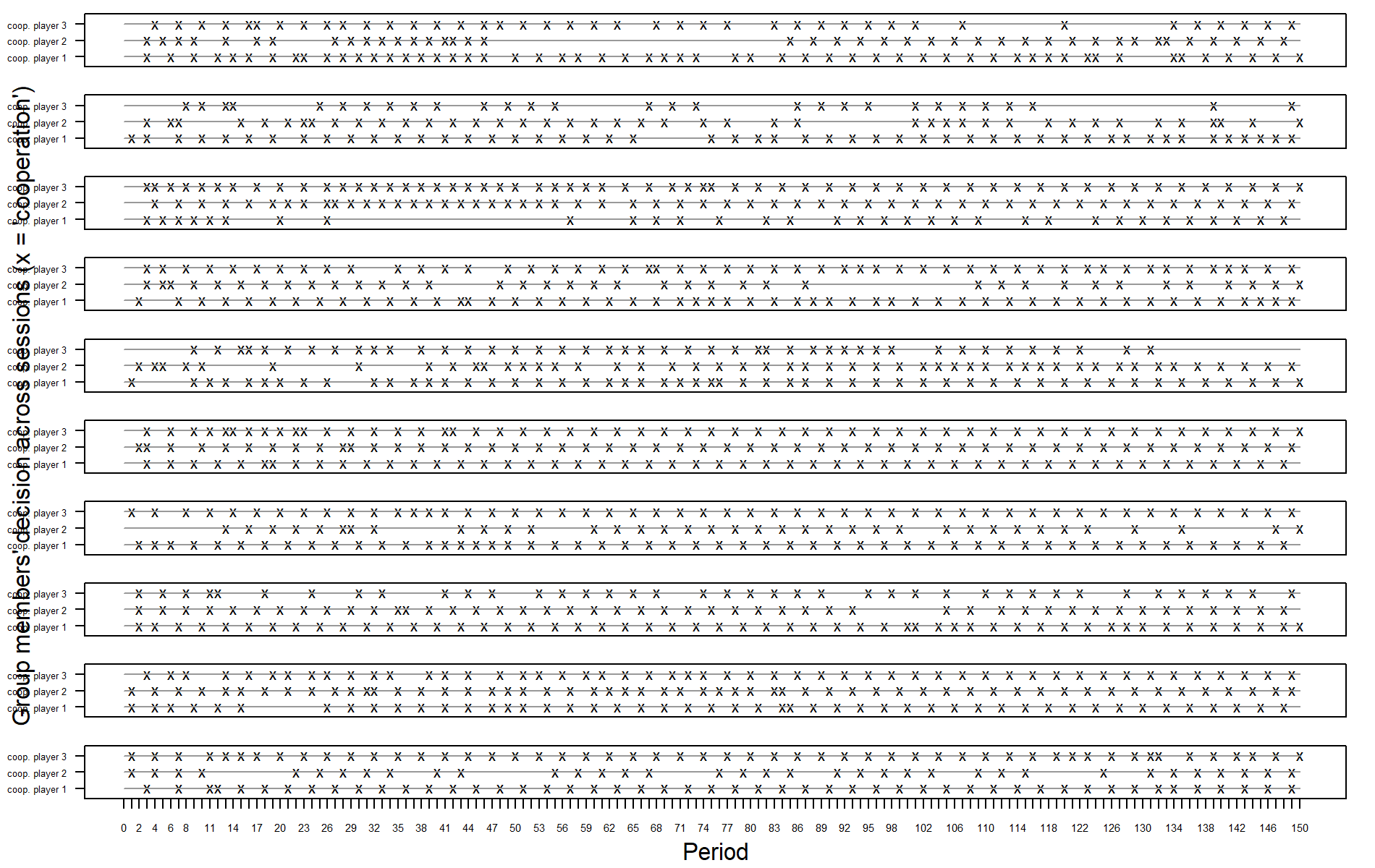
To gain further insight into LNI variance and thus the stability of emerging patterns, Figures 4 and 6 show two representative examples of simulation runs from the best fitting models of each model class. For each model run, an “x” denotes which of the three agents volunteered in a specific round.4 Furthermore, Figures 5 and 7 show all emerging cycles in the Markov-chains (or stable patterns) for the best fitting models of each model class that were stable in the last 20 rounds of a simulation run.5
In the asymmetric VOD (Figure 4), the example rounds of the ClassicQ model instance CQ.291 show that this model is the first to have consistent volunteering by a single agent (agent 1: the agent with the lowest costs from volunteering). The two runs show that between runs, the speed of learning can differ. Furthermore, Figure 5 shows that solitary volunteering by agent 1 and continuous abstention from volunteering by agents 2 and 3 is not only dominant (most occurring), but the only emerging pattern for ClassicQ in the asymmetric VOD. For the SequenceX model runs, agent 3 also learns to volunteer (Figure 4, SX.145, run 1). However, another agent (agent 2) also occasionally volunteers, thereby limiting the percentage of trials in which there is solitary volunteering. Furthermore, Figure 5 reveals that the dominant pattern for SequenceX in the asymmetric VOD is a form of turn-taking between two agents (1: \(\neg vvv\), 2/3: \(v\neg v\neg v\)), as shown in run 2 for SX.145 in Figure 4. Note that this is an efficient outcome that is not captured by the \(LNI\). For the VolunteerX model, the dominant pattern is solitary volunteering by agent 1 (see Figure 4, VX.239, run 1 and Figure 5). However, turn-taking between three agents can also be found. Therefore, although the forward-looking models (SequenceX, VolunteerX) can, in principle, learn the pattern, they do not do this consistently.
For the symmetric VOD (Figure 6 and 7), all three models seem to learn some patterns of turn-taking among all three agents. The SequenceX and VolunteerX models both can learn a (almost) perfect alternation (as is also observed in the behavioral experiment; see Diekmann & Przepiorka 2016). Note that alternation in the SequenceX model requires three different action sequences (\(\neg v\neg vv\), \(v\neg v\neg v\), \(\neg vv\neg v\)) differing in when to volunteer, as all three agents select a new action sequence at the same time (every third round). In contrast, alternation in the VolunteerX model requires the agents to coordinate when to start a single action sequence (\(¬v¬vv\)). Although, turn-taking between three agents it is the only stable pattern emerging for SequenceX and VolunteerX (see Figure 7), it can take up to 100 rounds to stabilize. That is, although these models produce better fits in the symmetric condition, they need on average more time to learn stable behavior compared to human participants. Furthermore, ClassicQ can show turn-taking with an alteration of \(\neg v\neg vv\) (Figure 6, CQ.110, top pattern). However, this typically does not entail all three agents (see Figure 6, CQ.110, run 1). The dominant pattern for ClassicQ in the symmetric condition remains some form of volunteering by a single agent (see Figure 6, CQ.110, run 2).
RQ2: Which model properties affect fit systematically
One interpretation of the results pertaining to RQ1 is that, in principle, different model classes can fit different aspects of the human data. This instigates the question what structural factors of the reinforcement models contributed to this fit. To this end, we analyzed the fit data generated by all the model instances (i.e., all parameter combinations) of the three model classes by means of multiple regression models. This allowed us to identify the direction and effect size of each parameter on model fit. The regression results are summarized in Table 3 (the full regression models are included in Tables 5 through 7 in the Appendix).
| Asymmetric | Symmetric | |||||
|---|---|---|---|---|---|---|
| ClassicQ | SequenceX | VolunteerX | ClassicQ | SequenceX | VolunteerX | |
| Discount rate (\(\gamma\)) | -- | - | - | - | - | -- |
| Learning rate (\(\alpha\)) | -- | - | 0 | 0 | - | + |
| Initial Q-value (\(\iota\)) | 0 | 0 | 0 | 0 | 0 | 0 |
| Exploration rate (\(\eta\)) | +++ | +++ | 0 | -- | 0 | ++ |
| Social behavior (\(S\)) | altruistic | altruistic | altruistic | selfish | altruistic | altruistic |
| "+" indicates improvement of model fit (lower RMSE) for higher parameter values. "-" indicate worse model fits for higher parameter values. The number of signs indicates effect size: +/- : \([2.0, 5.0)>\); ++/– : \([5.0, 10.0)\); +++/— : \(\geq 10.0\). Insignificant (p > .05) and/or small effects (effect size < 1.0) are denoted with “0”. For social behavior, the category with the better (significant) fit is indicated. | ||||||
For all models and in all conditions, better fits are produced when agents act myopically, favoring immediate rewards over potential future rewards (low \(\gamma\)). Furthermore, half of the models fare better when agents rely on experience (low \(\alpha\)) and exploration (large \(\eta\)), while most models produce better fit with altruistic reward expectations (i.e., maximizing group rather than individual reward). Especially the differences in parameter settings between conditions and models allow deeper insights about the learning process.
First, agents in the VolunteerX model class and the symmetric VOD condition produce better fit with the human data when they rely more on recent rewards (high \(\alpha\)), rather than earlier (accumulated) experience. Our interpretation is that this effect is due to the inconsistent length of action sequences between different state-action pair alternatives. As a result, agents need to coordinate (and thus constantly reconsider) two things: (a) the same (for altruistic agents optimal) strategy (\(Q(\emptyset; \neg v\neg vv)\)) and (b) staggered points in time (e.g., agent 1 = round 1, agent 2 = round 2, agent 3 = round 3). This requires thorough exploration of the state-action pairs, while relying too much on experience before having coordinated on action strategies and time points may cause altruistic agents to get stuck in suboptimal outcomes for the group as a whole (e.g., turn-taking between 2 agents).
Second, agents in the ClassicQ model class and the symmetric VOD condition produce better fit with the human data, when they favor exploitation over exploration (low \(\eta\)) while acting selfishly (i.e., considering only own rewards). Our interpretation is that this effect occurs because the expected selfish rewards provide a more salient optimum in the symmetric condition for all agents (e.g., \(vv\rightarrow v:30 + 30 + 30 = 90\); \(\neg v\neg v \rightarrow v:80 + 80 + 30 = 190\); so the difference between the two is 100) when compared to the expected altruistic rewards of the agent with the lowest costs to volunteer in the asymmetric condition (e.g., \(vv\rightarrow v: 70 + 70 + 70 = 210\); \(\neg v\neg v \rightarrow v:80 + 80 + 70 = 230\); so the difference between the two is only 20). The former allows to exploit quickly (low \(\eta\)), while the latter requires exploration of the agent with the lowest costs to find the more subtle differences in payoffs.
In summary, the results show four main findings. First, no single model produces best fits in both conditions. Second, quick coordination relies on myopic agents favoring current reward rather than working towards potentially higher gains in the future (low \(\gamma\)). Third, settings of other parameters differ between model classes and conditions. Fourth, coordination requires less exploration when optima are salient.
General Discussion
We investigated whether reinforcement learning can provide a unifying computational mechanism to explain the emergence of conventions in the repeated volunteer’s dilemma (VOD). Feedback and learning are at the core of reinforcement learning (Sutton & Barto 2018), and an important factor considered to be involved in learning to act in the real world (Spike et al. 2017). Our results suggest that reinforcement learning models can fit, and thereby describe, the emergence of conventions in small human groups.
Furthermore, we find that the exact structure and details of the model matter, as there was not one model class that provided a best fit in all conditions. While all three model classes (ClassicQ, SequenceX, VolunteerX) are based on Q-Learning, and thus favor the best performing action in a given state, they differ in how actions and states are defined (see Figure 2). ClassicQ follows a backward-looking perspective, where a state is defined by the two previously performed actions, and actions performed in the current round consist of volunteering and not volunteering. In contrast, SequenceX and VolunteerX follow a forward-looking perspective by defining a sequence of actions (consisting of volunteering, not volunteering), selected whenever there are no more actions left to be performed.
In the asymmetric condition, ClassicQ had the best fit with the empirical data. Our interpretation is that this fit emerged due to the combination of model properties and a salient external reward structure. Specifically, ClassicQ has a structural advantage. That is, ClassicQ can make a decision each round (see Figure 2, only black states connected with black arrows), rather than up to every third round like SequenceX and VolunteerX. Moreover, each time there is only a decision between two actions (to volunteer or to not volunteer), rather than 8 action strategies for SequenceX, or 4 action strategies for VolunteerX (see Figure 2, one single black state with 8 or 4 black outgoing arrows to orange states). When combined with the salient reward structure of the asymmetric VOD (one agent has lower costs to volunteer), ClassicQ has a relatively easy learning problem, compared to the other two model classes: a binary choice with feedback in each round. This aligns with the principle in Spike et al. (2017) that a salient reward is essential for behavior emergence and in line with more recent behavioral data from experiments with the asymmetric VOD (Przepiorka et al. 2021).
In the symmetric condition, VolunteerX has the overall best fit, closely followed by SequenceX. VolunteerX also has the best fitting model when both the symmetric and asymmetric condition are considered. Our interpretation of this result is that VolunteerX combines the advantages of two mutually impeding model concepts: structure through forward-looking action sequences and timely assessment of success. As for the first advantage, VolunteerX (and SequenceX) retains contextual structure by defining forward-looking sequences of consecutive actions. This differs from the ClassicQ model class, which lacks the possibility to actively test combinations of actions. In contrast to SequenceX, which considers all possible action sequences of length 3, VolunteerX defines when to volunteer (i.e., in the 1st, 2nd, or 3rd round, or not at all). This reduces the number of state-action pairs that the model needs to consider from eight in SequenceX to only four in VolunteerX. Consequently, VolunteerX learns to coordinate relatively quickly in the difficult learning task of the symmetric condition, where turn-taking between three agents is dominant in the experimental data but ambiguous regarding who should start the sequence.
The differences in model fit between the various model classes suggest that there are different strategies in play when humans form conventions in the VOD. In simple scenarios with salient optima immediate evaluation of single actions lead to quick coordination. In more complex and ambiguous scenarios inferring structure from the problem helps to coordinate joint actions. Thus, contextual cues may help humans to select potentially fruitful and successfully apply coordination strategies.
Concerning the parameters (RQ2), there is again some variation between model classes. However, a commonality for all model classes and all conditions is that better fits are obtained when agents act myopically, favoring current over expected future rewards (i.e., have low discount rate \(\gamma\)). Furthermore, most models fare better when agents rely on experience (low \(\alpha\)). Finally, most models produce better fits with altruistic reward expectations. That is, agents coordinate quicker, and patterns are more stable, when agents maximize rewards for the entire group rather than considering only individual benefits. In the asymmetric VOD, altruistic reward expectations create a salient optimum for solitary volunteering of the agent with the lowest costs to volunteer. In the symmetric VOD, altruistic reward expectations create the same expected reward for all agents, thus facilitating patterns that allow equal distribution of costs (i.e., turn-taking). The results, therefore, suggest that human participants in the repeated VOD favor immediate rewards, rely on experience, and consider rewards for the entire group.
These predictions are qualitatively consistent with other cognitive models of convention emergence. Good fits, for example, were produced in various two-person coordination games when agents acted myopically, giving less weight to future prospects for success (e.g., Zschache 2016, 2017). Furthermore, conventions emerged with comparably low cognitive skill requirements. That is, agents do not actively consider the decisions of others, but observe and aggregate personal rewards over time (e.g., Zschache 2016, 2017). In contrast to earlier work, our good fits also benefit from inherent parameters of the general reinforcement learning mechanism, rather than mechanisms behind memory and forgetting to model convention emergence (Collins et al. 2016; Gonzalez et al. 2015; Juvina et al. 2015; Stevens et al. 2016). The underlying memory mechanism of some models (e.g., Anderson et al. 2004), also predicts that memories (and associated behaviors) are learned faster when actions are consistent and observed frequently (Anderson & Schooler 1991). This aligns with our observation of low \(\gamma\) (focus on present) and low \(\alpha\) (consistent learning).
We also showed that in line with Zschache (2016) complete neglect of other agents can explain experimental data (selfish ClassicQ in the symmetric VOD). However, considering rewards of others (altruism) produces better fits with the experimental data in general. This in turn corresponds to the Roth-Erev model (Roth & Erev 1995), which suggests that knowing each other’s payoffs and salient optima lead faster to perfect equilibria. Our results additionally suggest that considering contextual clues (e.g., reward structure) for strategy design (e.g., sequences of actions) and strategy selection (e.g., favoring equal distribution of costs) may help to coordinate more quickly when optima are less salient (e.g., symmetric VOD).
Future work could test if our qualitative model predictions hold. Specifically, our results suggest that stable social conventions are more likely to emerge when the rewards for adhering to the convention are not delayed, when rewards are provided reliably so that decisions can rely on experience, and when contextual clues, such as reward structures of the entire group, can be integrated into the action selection process. Put differently, conventions will take longer to emerge, when rewards are delayed and when the rewards for joint actions do not create salient optima. Applying and comparing these insights to additional settings would furthermore allow to generalize our findings; a necessary step towards the definition of a formal theory of learning in the emergence of conventions.
Notes
- Note that despite the use of noise in the calculation of which action to select, the actual Q-value is updated based on experience, as expressed in Equation 1.↩︎
- Note that the total number of 150 rounds is about three times the number of rounds of the experimental study by Diekmann & Przepiorka (2016). In a pilot study we compared pattern emergence and stability with an increasing number of rounds (50, 100, 150, 200, 250, 500). It showed that agents require about 100 rounds to coordinate in the symmetric condition (fewer rounds in the asymmetric condition). Simulations with more than 100 rounds, however, showed that the emerging coordination patterns are not necessarily stable, while simulations with more than 150 rounds hardly ever showed pattern changes after the 150 rounds. Simulations with 150 rounds therefore combine two things: agents are able to learn to coordinate and emerging patterns are stable.↩︎
- See Table 4 in the Appendix for corresponding parameter settings.↩︎
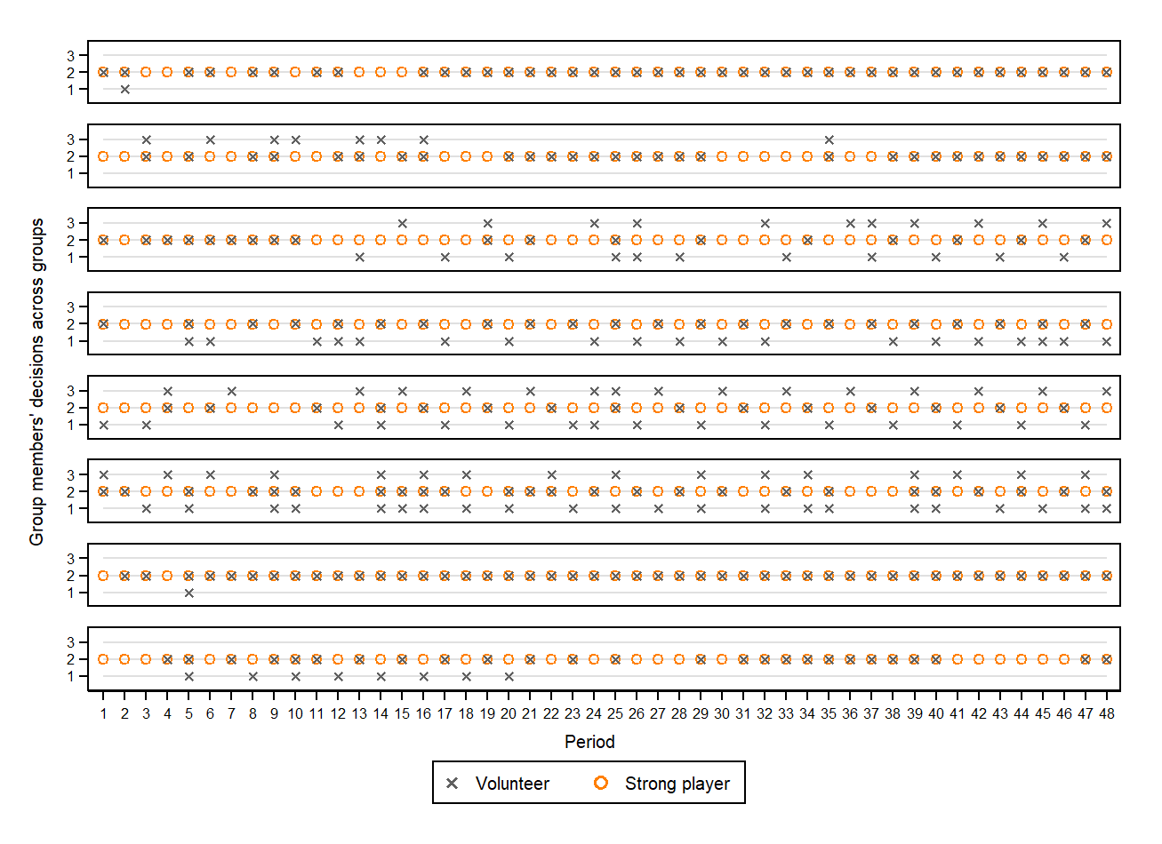
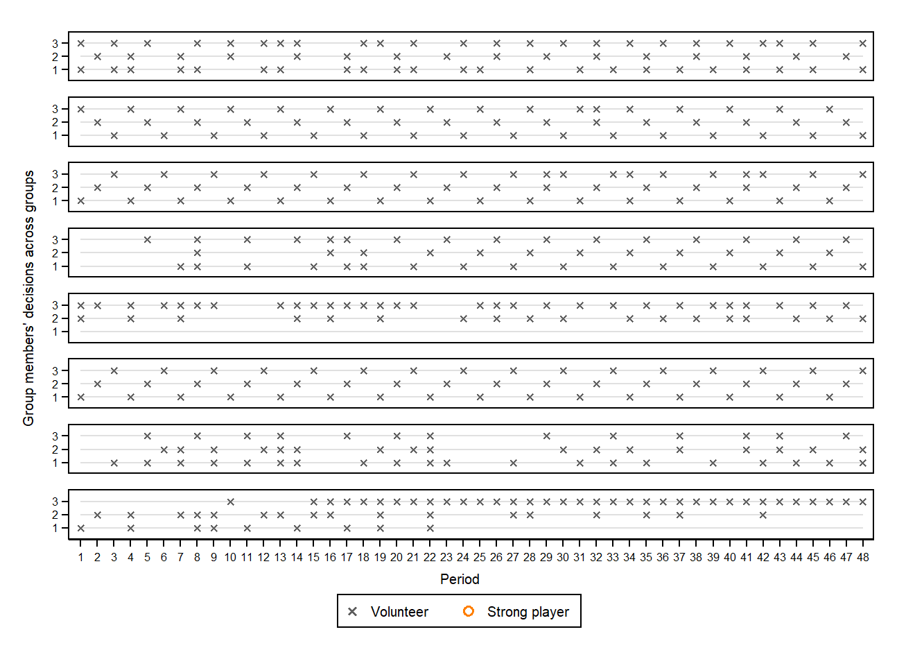
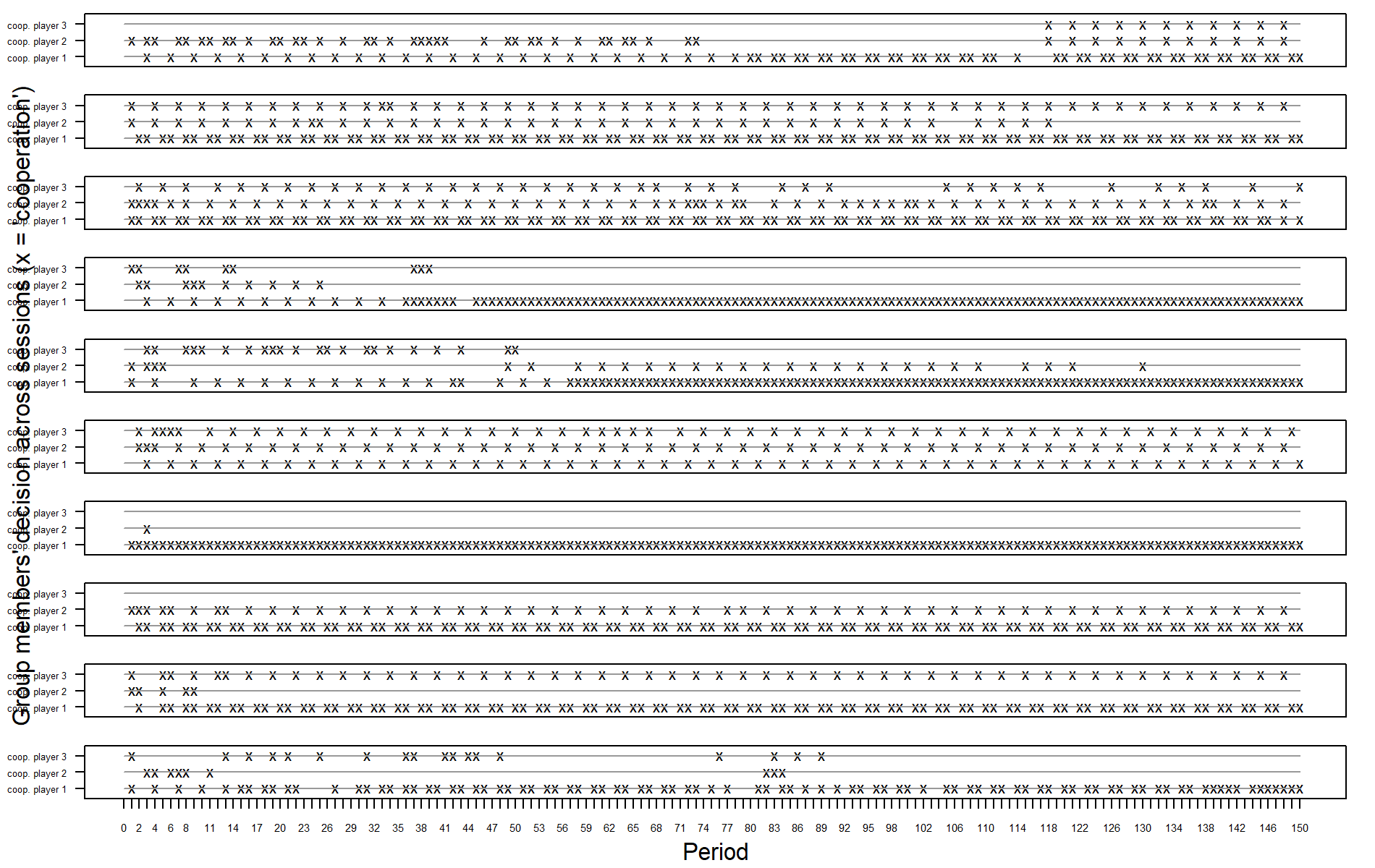
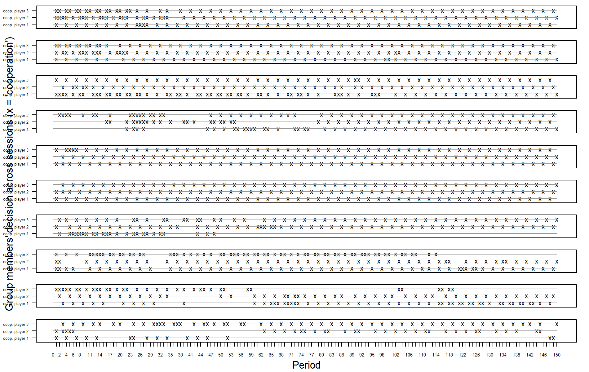
- For comparison purposes, examples of human behavioral patterns that emerge in the symmetric and asymmetric VOD are shown in the Appendix in Figures 10 and 11, respectively.↩︎
- All emerging patterns of the models producing best fits are shown in the Appendix in Figures 12- 17.↩︎
Model Documentation
The R code of the simulation to generate and analyze the data is available under the GPLv3 license in the GitHub repository, https://github.com/hnunner/relavod, version: v1.0.4., commit: 72d258e, DOI:10.5281/zenodo.4742547 (Nunner 2021).| ClassicQ | SequenceX | VolunteerX | ||||||
|---|---|---|---|---|---|---|---|---|
| CQ.47 | CQ.291 | CQ.110 | SX.145 | SX.182 | VX.157 | VX.239 | VX.213 | |
| Best fit (RMSE) of this model type for: | Comb | Asym | Sym | Comb and Asym | Sym | Comb | Asym | Sym | Best fit (RMSE) across all models for | Asym | Comb | Sym |
| Variables | ||||||||
| Social preference | selfish | selfish | selfish | selfish | selfish | selfish | selfish | selfish |
| Initial Q-values | 43.33 | 43.33 | 43.33 | 67.5 | 67.5 | 67.5 | 67.5 | 67.5 |
| Learning rate | 0.4 | 0.4 | 0.65 | 0.3 | 0.45 | 0.35 | 0.7 | 0.6 |
| Discount rate | 0.6 | 0.7 | 1 | 0.55 | 0.75 | 0.6 | 0.85 | 0.65 |
| Explor. rate | 0.1 | 0.2 | 0.1 | 0.1 | 0.1 | 0.1 | 0.1 | 0.1 |
| Constants | ||||||||
| Explor. V. Exploit. | \(\eta\)-noise | \(\eta\)-noise | \(\eta\)-noise | \(\eta\)-noise | \(\eta\)-noise | \(\eta\)-noise | \(\eta\)-noise | \(\eta\)-noise |
| Cooperation Ratio | 0.33 | 0.33 | 0.33 | 0.33 | 0.33 | 0.33 | 0.33 | 0.33 |
| Explor. Decrease | 1 | 1 | 1 | 1 | 1 | 1 | 1 | 1 |
| Actions per state | 2 | 2 | 2 | NA | NA | NA | NA | NA |
| Agents per state | 1 | 1 | 1 | NA | NA | NA | NA | NA |
| Exp size | NA | NA | NA | 3 | 3 | 3 | 3 | 3 |
| Model fit when looking at asymmetric and symmetric combined | ||||||||
| RMSE | 20.07 | 24.01 | 32.24 | 19.57 | 26.29 | 16.51 | 18.11 | 23.87 |
| \(R^{2}\) | 0.49 | 0.42 | 0.13 | 0.26 | 0.19 | 0.53 | 0.46 | 0.26 |
| Model fit for asymmetric condition only | ||||||||
| RMSE | 4.18 | 3.87 | 35.68 | 25.02 | 37.70 | 15.59 | 13.47 | 33.08 |
| \(R^{2}\) | 0.99 | 0.98 | 0.04 | 0.04 | 0.01 | 0.57 | 0.69 | 0.02 |
| Model fit for symmetric condition only | ||||||||
| RMSE | 32.89 | 36.00 | 26.44 | 17.63 | 6.77 | 17.40 | 16.30 | 5.11 |
| \(R^{2}\) | 0.07 | 0.14 | 0.08 | 0.51 | 0.93 | 0.52 | 0.53 | 0.97 |
| Notes: Experimental variables were varied as follows: (1) social preferences: selfish vs altruistic; (2) initial propensities: 43.33 vs 67.5; (3) learning rate: 0.20 - 0.70 in steps of 0.05; (4) discount rate 0.50 - 1.00 in steps of 0.05; (5) exploration rate: 0.1 vs 0.2. | ||||||||
| Symmetric | Asymmetric | |||
|---|---|---|---|---|
| Model 1 | Model 2 | Model 1 | Model 2 | |
| Intercept | 34.94 (0.06)*** | 34.94 (0.06)*** | 26.58 (0.26)*** | 26.58 (0.20)*** |
| Discount rate (\(\gamma\)) | 3.99 (0.40)*** | 3.99 (0.36)*** | 8.01 (1.61)*** | 8.01 (1.28)*** |
| Learning rate (\(\alpha\)) | 0.24 (0.40) | 0.24 (0.36) | 5.02 (1.61)** | 5.02 (1.28)*** |
| Initial Q-values (\(\iota\)) | 0.03 (0.01)*** | 0.03 (0.00)*** | 0.02 (0.02) | 0.02 (0.02) |
| Exploration rate (\(\eta\)) | 5.59 (1.25)*** | 5.59 (1.15)*** | -25.21 (5.10)*** | -25.21 (4.06)*** |
| Social behavior (\(S\)) | 2.08 (0.13)*** | 2.08 (0.11)*** | -20.65 (0.51)*** | -20.65 (0.41)*** |
| Interaction effects | ||||
| \(\gamma\) \(\times\) \(\alpha\) | -1.79 (2.29) | 9.19 (8.11) | ||
| \(\gamma\) \(\times\) \(\iota\) | 0.14 (0.03)*** | -1.33 (0.11)*** | ||
| \(\gamma\) \(\times\) \(\eta\) | -9.38 (7.25) | -150.73 (25.65)*** | ||
| \(\gamma\) \(\times\) \(S\) | 9.11 (0.73)*** | 19.77 (2.56)*** | ||
| \(\alpha\) \(\times\) \(i\) | 0.02 (0.03) | 0.22 (0.11)* | ||
| \(\alpha\) \(\times\) \(\eta\) | 1.89 (7.25) | 7.31 (25.65) | ||
| \(\alpha\) \(\times\) \(S\) | -1.43 (0.73)* | 6.29 (2.56)* | ||
| \(\iota\) \(\times\) \(\eta\) | 0.19 (0.09)* | 2.81 (0.34)*** | ||
| \(\iota\) \(\times\) \(S\) | -0.01 (0.01) | -0.29 (0.03)*** | ||
| \(\eta\) \(\times\) \(S\) | -4.60 (2.29)* | -103.95 (8.11)*** | ||
| Adj. R2 | 0.30 | 0.42 | 0.64 | 0.77 |
| Num. Obs. | 968 | 968 | 968 | 968 |
| RMSE | 1.95 | 1.78 | 7.94 | 6.31 |
| ***p < 0.001, **p < 0.01, *p < 0.05. Note: Lower RMSEs indicate better fit with empirical data. Thus, negative signs indicate better fit for increasing values. \(S\) has been converted to 1 (altruistic) and 2 (selfish). | ||||
| Symmetric | Asymmetric | |||
|---|---|---|---|---|
| Model 1 | Model 2 | Model 1 | Model 2 | |
| Intercept | 30.56 (0.13)*** | 30.56 (0.11)*** | 39.15 (0.14)*** | 39.15 (0.14)*** |
| Discount rate (\(\gamma\)) | 5.35 (0.83)*** | 5.35 (0.71)*** | 2.23 (0.92)* | 2.23 (0.85)** |
| Learning rate (\(\alpha\)) | -3.31 (0.83)*** | -3.31 (0.71)*** | -0.00 (0.92) | -0.00 (0.85) |
| Initial Q-values (\(\iota\)) | -0.11 (0.01)*** | -0.11 (0.01)*** | -0.06 (0.01)*** | -0.06 (0.01)*** |
| Exploration rate (\(\eta\)) | -8.39 (2.62)** | -8.39 (2.25)*** | 2.76 (2.89) | 2.76 (2.70) |
| Social behavior (\(S\)) | -6.64 (0.26)*** | -6.64 (0.23)*** | -4.87 (0.29)*** | -4.87 (0.27)*** |
| Interaction effects | ||||
| \(\gamma\) \(\times\) \(\alpha\) | 11.43 (4.51)* | -7.54 (5.40) | ||
| \(\gamma\) \(\times\) \(\iota\) | -0.08 (0.06) | 0.01 (0.07) | ||
| \(\gamma\) \(\times\) \(\eta\) | -52.65 (14.25)*** | -48.75 (17.08)** | ||
| \(\gamma\) \(\times\) \(S\) | 11.49 (1.43)*** | 6.68 (1.71)*** | ||
| \(\alpha\) \(\times\) \(\iota\) | -0.34 (0.06)*** | -0.03 (0.07) | ||
| \(\alpha\) \(\times\) \(\eta\) | 45.86 (14.25)** | 20.96 (17.08) | ||
| \(\alpha\) \(\times\) \(S\) | -8.91 (1.43)*** | 2.29 (1.71) | ||
| \(\iota\) \(\times\) \(\eta\) | 1.64 (0.19)*** | 1.79 (0.22)*** | ||
| \(\iota\) \(\times\) \(S\) | -0.16 (0.02)*** | -0.17 (0.02)*** | ||
| \(\eta\) \(\times\) \(S\) | 22.02 (4.51)*** | -5.68 (5.40) | ||
| Adj. R2 | 0.46 | 0.60 | 0.24 | 0.34 |
| Num. Obs. | 968 | 968 | 968 | 968 |
| RMSE | 4.07 | 3.51 | 4.50 | 4.20 |
| ***p < 0.001, **p < 0.01, *p < 0.05. Note: Lower RMSEs indicate better fit with empirical data. Thus, negative signs indicate better fit for increasing values. \(S\) has been converted to 1 (altruistic) and 2 (selfish). | ||||
| Symmetric | Asymmetric | |||
|---|---|---|---|---|
| Model 1 | Model 2 | Model 1 | Model 2 | |
| Intercept | 32.82 (0.13)*** | 32.82 (0.11)*** | 41.79 (0.10)*** | 41.79 (0.09)*** |
| Discount rate (\(\gamma\)) | 4.56 (0.81)*** | 4.56 (0.72)*** | 4.80 (0.65)*** | 4.80 (0.59)*** |
| Learning rate (\(\alpha\)) | 2.82 (0.81)*** | 2.82 (0.72)*** | 2.56 (0.65)*** | 2.56 (0.59)*** |
| Initial Q-values (\(\iota\)) | -0.09 (0.01)*** | -0.09 (0.01)*** | -0.10 (0.01)*** | -0.10 (0.01)*** |
| Exploration rate (\(\eta\)) | -1.91 (2.55) | -1.91 (2.29) | -15.65 (2.06)*** | -15.65 (1.88)*** |
| Social behavior (\(S\)) | -4.89 (0.25)*** | -4.89 (0.23)*** | -3.90 (0.21)*** | -3.90 (0.19)*** |
| Interaction effects | ||||
| \(\gamma\) \(\times\) \(\alpha\) | -10.53 (4.58)* | -12.06 (3.75)** | ||
| \(\gamma\) \(\times\) \(\iota\) | -0.12 (0.06)* | 0.05 (0.05) | ||
| \(\gamma\) \(\times\) \(\eta\) | -45.72 (14.47)** | -23.40 (11.86)* | ||
| \(\gamma\) \(\times\) \(S\) | 3.59 (1.45)* | 7.77 (1.19)*** | ||
| \(\alpha\) \(\times\) \(\iota\) | 0.21 (0.06)*** | 0.12 (0.05)* | ||
| \(\alpha\) \(\times\) \(\eta\) | -25.37 (14.47) | -4.38 (11.86) | ||
| \(\alpha\) \(\times\) \(S\) | 3.01 (1.45)* | 4.37 (1.19)*** | ||
| \(\iota\) \(\times\) \(\eta\) | 2.55 (0.19)*** | 0.10 (0.16) | ||
| \(\iota\)) \(\times\) \(S\) | -0.06 (0.02)** | -0.15 (0.02)*** | ||
| \(\eta\) \(\times\) \(S\) | 8.86 (4.58) | -20.96 (3.75)*** | ||
| Adj. R2 | 0.33 | 0.46 | 0.39 | 0.49 |
| Num. Obs. | 968 | 968 | 968 | 968 |
| RMSE | 3.96 | 3.56 | 3.20 | 2.92 |
| ***p < 0.001, **p < 0.01, *p < 0.05. Note: Lower RMSEs indicate better fit with empirical data. Thus, negative signs indicate better fit for increasing values. \(S\) has been converted to 1 (altruistic) and 2 (selfish). | ||||
References
ANDERSON, J. R. (2007). How Can the Human Mind Occur in the Physical Universe? NewYork, NY: Oxford University Press. [doi:10.1093/acprof:oso/9780195324259.003.0006]
ANDERSON, J. R., Bothell, D., Byrne, M. D., Douglass, S., Lebiere, C., & Qin, Y. (2004). An integrated theory of the mind. Psychological Review, 111(4), 1036–1060. [doi:10.1037/0033-295x.111.4.1036]
ANDERSON, J. R., & Schooler, L. (1991). Reflections of the environment in memory. Psychological Science, 2(6), 396–408. [doi:10.1111/j.1467-9280.1991.tb00174.x]
ANDREONI, J. (1995). Cooperation in public-Goods experiments – Kindness or confusion. American Economic Review, 85(4), 891–904.
CAMERER, C. F. (2003). Behavioral Game Theory. Princeton, NJ: Princeton University Press.
CENTOLA, D., & Baronchelli, A. (2015). The spontaneous emergence of conventions: An experimental study of cultural evolution. Proceedings of the National Academy of Sciences, 112(7), 1989–1994. [doi:10.1073/pnas.1418838112]
CHAUDHURI, A. (2011). Sustaining cooperation in laboratory public goods experiments: A selective survey of the literature. Experimental Economics, 14(1), 47–83. [doi:10.1007/s10683-010-9257-1]
COLLINS, M. G., Juvina, I., & Gluck, K. A. (2016). Cognitive model of trust dynamics predicts human behavior within and between two games of strategic interaction with computerized confederate agents. Frontiers in Psychology, 7, 49. [doi:10.3389/fpsyg.2016.00049]
DIEKMANN, A. (1985). Volunteer’s dilemma. Journal of Conflict Resolution, 29(4), 605–610. [doi:10.1177/0022002785029004003]
DIEKMANN, A. (1993). Cooperation in an asymmetric volunteer’s dilemma game: Theory and experimental evidence. International Journal of Game Theory, 22(1), 75–85. [doi:10.1007/bf01245571]
DIEKMANN, A., & Przepiorka, W. (2016). "Take One for the Team!" individual heterogeneity and the emergence of latent norms in a volunteer’s dilemma. Social Forces, 93(3), 1309–1333. [doi:10.1093/sf/sov107]
DIJKSTRA, J., & Bakker, D. M. (2017). Relative power: Material and contextual elements of efficacy in social dilemmas. Social Science Research, 62, 255–271. [doi:10.1016/j.ssresearch.2016.08.011]
FISCHBACHER, U., Gächter, S., & Fehr, E. (2011). Are people conditionally cooperative? Evidence from a public goods experiment. Economics Letters, 71(3), 397–404. [doi:10.1016/s0165-1765(01)00394-9]
GAGNIUC, P. A. (2017). Markov Chains: From Theory to Implementation and Experimentation. Hoboken, NJ: John Wiley & Sons. [doi:10.1002/9781119387596]
GONZALEZ, C., Ben-Asher, N., Martin, J. M., & Dutt, V. (2015). A cognitive model of dynamic cooperation with varied interdependency information. Cognitive Science, 39(3), 457–495. [doi:10.1111/cogs.12170]
GUALA, F., & Mittone, L. (2010). How history and convention create norms: An experimental study. Journal of Economic Psychology, 31(4), 749–756. [doi:10.1016/j.joep.2010.05.009]
HARSANYI, J. C., & Selten, R. (1988). A General Theory of Equilibrium Selection in Games. Cambridge, MA: MIT Press.
HAUSER, O. P., Hilbe, C., Chatterjee, K., & Nowak, M. A. (2019). Social dilemmas among unequals. Nature, 572, 524–527. [doi:10.1038/s41586-019-1488-5]
HAWKINS, R. X. D., Goodman, N. D., & Goldstone, R. L. (2019). The emergence of social norms and conventions. Trends in Cognitive Sciences, 23(2), 158–169. [doi:10.1016/j.tics.2018.11.003]
HELBING, D., Schönhof, M., Stark, H. U., & Hołyst, J. A. (2005). How individuals learn to take turns: Emergence of alternating cooperation in a congestion game and the prisoner’s dilemma. Advances in Complex Systems, 8(01), 87–116. [doi:10.1142/s0219525905000361]
HERRNSTEIN, R. J., Loewenstein, G. F., Prelec, D., & Vaughan Jr, W. (1993). Utility maximization and melioration: Internalities in individual choice. Journal of Behavioral Decision Making, 6(3), 149–185. [doi:10.1002/bdm.3960060302]
HERRNSTEIN, R. J., & Vaughan, W. (1980). 'Melioration and behavioral allocation.' In J. E. R. Staddon (Ed.), Limits to Action: The Allocation of Individual Behavior (pp. 143–176). Cambridge, MA: Academic Press. [doi:10.1016/b978-0-12-662650-6.50011-8]
IZQUIERDO, L. R., IZQUIERDO, S. S., Gotts, N. M., & Polhill, J. G. (2007). Transient and asymptotic dynamics of reinforcement learning in games. Games and Economic Behavior, 61(2), 259–276. [doi:10.1016/j.geb.2007.01.005]
IZQUIERDO, S. S., IZQUIERDO, L. R., & Gotts, N. M. (2008). Reinforcement learning dynamics in social dilemmas. Journal of Artificial Societies and Social Simulation, 11(2), 1: http://jasss.soc.surrey.ac.uk/11/2/1.html.
JUVINA, I., Lebiere, C., & Gonzalez, C. (2015). Modeling trust dynamics in strategic interaction. Journal of Applied Research in Memory and Cognition, 4(3), 197–211. [doi:10.1016/j.jarmac.2014.09.004]
KUBE, S., Schaube, S., Schildberg-Hörisch, H., & Khachatryan, E. (2015). Institution formation and cooperation with heterogeneous agents. European Economic Review, 78, 248–268. [doi:10.1016/j.euroecorev.2015.06.004]
LAIRD, J. E. (2012). The Soar Cognitive Architecture. Cambridge, MA: MIT Press.
LAU, S. H. P., & Mui, V. L. (2012). Using turn taking to achieve intertemporal cooperation and symmetry in infinitely repeated 2 × 2 games. Theory and Decision, 72(2), 167–188. [doi:10.1007/s11238-011-9249-4]
LEWIS, D. (1969). Convention: A Philosophical Study. Cambridge, MA: Harvard University Press.
MACY, M. W., & Flache, A. (2002). Learning dynamics in social dilemmas. Proceedings of the National Academy of Sciences, 99(suppl 3), 7229–7236. [doi:10.1073/pnas.092080099]
MAZUR, J. E. (1981). Optimization theory fails to predict performance of pigeons in a two-response situation. Science, 214(4522), 823–825. [doi:10.1126/science.7292017]
MILINSKI, M., Sommerfeld, R. D., Krambeck, H. J., Reed, F. A., & Marotzke, J. (2008). The collective-risk social dilemma and the prevention of simulated dangerous climate change. Proceedings of the National Academy of Sciences, 105(7), 2291–2294. [doi:10.1073/pnas.0709546105]
NEWELL, A. (1990). Unified Theories of Cognition. Cambridge, MA: Harvard University Press.
NUNNER, H. (2021). ReLAVOD: Reinforcement learning agents in the volunteer’s dilemma. Available at: https://github.com/hnunner/relavod, version: v1.0.4., commit: 72d258e.
OTTEN, K., Buskens, V., Przepiorka, W., & Ellemers, N. (2020). Heterogeneous groups cooperate in public good problems despite normative disagreements about individual contribution levels. Scientific Reports, 10, 16702. [doi:10.1038/s41598-020-73314-7]
PRZEPIORKA, W., Bouman, L., & de Kwaadsteniet, E. W. (2021). The emergence of conventions in the repeated volunteer’s dilemma: The role of social value orientation, payoff asymmetries and focal points. Social Science Research, 93, 102488. [doi:10.1016/j.ssresearch.2020.102488]
PRZEPIORKA, W., & Diekmann, A. (2013). Individual heterogeneity and costly punishment: A volunteer’s dilemma. Social Science ResearchProceedings of the Royal Society B, 280(1759), 20130247. [doi:10.1098/rspb.2013.0247]
PRZEPIORKA, W., & Diekmann, A. (2018). Heterogeneous groups overcome the diffusion of responsibility problem in social norm enforcement. PLoS ONE, 13(11), e0208129. [doi:10.1371/journal.pone.0208129]
PRZEPIORKA, W., Székely, A., Andrighetto, G., Diekmann, A., & Tummolini, L. (2022). How norms emerge from conventions (and change). Unpublished manuscript, Department of Sociology/ICS, Utrecht University, the Netherlands.
RAPOPORT, A., & Suleiman, R. (1993). Incremental contribution in step-Level public goods games with asymmetric players. Organizational Behavior and Human Decision Processes, 55(2), 171–194. [doi:10.1006/obhd.1993.1029]
ROTH, A. E., & Erev, I. (1995). Learning in extensive-form games: Experimental data and simple dynamic models in the intermediate term. Games and Economic Behavior, 8(1), 164–212. [doi:10.1016/s0899-8256(05)80020-x]
SCHULTZ, W., Dayan, P., & Montague, P. R. (1997). A neural substrate of prediction and reward. Science, 275(5306), 1593–1599. [doi:10.1126/science.275.5306.1593]
SIMPSON, B., & Willer, R. (2015). Beyond altruism: Sociological foundations of cooperation and prosocial behavior. Annual Review of Sociology, 41, 43–63. [doi:10.1146/annurev-soc-073014-112242]
SPIKE, M., Stadler, K., Kirby, S., & Smith, K. (2017). Minimal requirements for the emergence of learned signaling. Cognitive Science, 41(3), 623–658. [doi:10.1111/cogs.12351]
STEVENS, C. A., Taatgen, N. A., & Cnossen, F. (2016). Instance-Based models of metacognition in the prisoner’s dilemma. Topics in Cognitive Science, 8(1), 322–334. [doi:10.1111/tops.12181]
SUGDEN, R. (1986). The Economics of Rights, Co-operation, and Welfare.. Oxford: Basil Blackwell.
SUN, X., Zhao, X., & Robaldo, L. (2017). Ali Baba and the Thief, convention emergence in games. Journal of Artificial Societies and Social Simulation, 20(3), 6: http://jasss.soc.surrey.ac.uk/20/3/6.html. [doi:10.18564/jasss.3421]
SUTTON, R., & Barto, A. G. (2018). Reinforcement Learning: An Introduction (2nd ed.). Cambridge, MA: MIT Press.
TUMMOLINI, L., Andrighetto, G., Castelfranchi, C., & Conte, R. (2013). A convention or (tacit) agreement betwixt us: On reliance and its normative consequences. Synthese, 190, 585–618. [doi:10.1007/s11229-012-0194-8]
TUNNEY, R. J., & Shanks, D. R. (2002). A re‐examination of melioration and rational choice. Journal of Behavioral Decision Making, 15(4), 291–311. [doi:10.1002/bdm.415]
VAN de Kragt, A. J. C., Orbell, J. M., & Dawes, R. M. (1983). The minimal contributing set as a solution to public goods problems. American Political Science Review, 77(1), 112–122. [doi:10.2307/1956014]
VAN Dijk, E., & Wilke, H. (1995). Coordination rules in asymmetric social dilemmas: A comparison between public good dilemmas and resource dilemmas. Journal of Experimental Social Psychology, 31(1), 1–27. [doi:10.1006/jesp.1995.1001]
VAUGHAN Jr, W. (1981). Melioration, matching, and maximization. Journal of the Experimental Analysis of Behavior, 36(2), 141–149. [doi:10.1901/jeab.1981.36-141]
WATKINS, C. J., & Dayan, P. (1992). Q-learning. Machine Learning, 8(3–4), 279–292. [doi:10.1023/a:1022676722315]
YOUNG, H. P. (1993). The evolution of conventions. Econometrica, 61(1), 57–84.
ZSCHACHE, J. (2016). Melioration learning in two-Person games. PLoS ONE, 11(11), e0166708. [doi:10.1371/journal.pone.0166708]
ZSCHACHE, J. (2017). The explanation of social conventions by melioration learning. Journal of Artificial Societies and Social Simulation, 20(3), 1: http://jasss.soc.surrey.ac.uk/20/3/1.html. [doi:10.18564/jasss.3428]