Hybrid Approach for Modelling the Uptake of Residential Solar PV Systems, with Case Study Application in Melbourne, Australia

, , ,
and
aSwinburne University of Technology, Australia; bCSIRO Land and Water, Australia
Journal of Artificial
Societies and Social Simulation 25 (4) 2
<https://www.jasss.org/25/4/2.html>
DOI: 10.18564/jasss.4921
Received: 02-Dec-2021 Accepted: 23-Aug-2022 Published: 31-Oct-2022
Abstract
Understanding the processes of residential solar PV uptake is critical to developing planning and policy energy transition pathways. This paper outlines a novel hybrid Agent-Based-Modelling/statistical adoption prediction framework that addresses several drawbacks in current modelling approaches. Specifically, we extend the capabilities of similar previous models and incorporate empirical data, behavioural theory, social networks and explicitly considers the spatial context. We provide empirical data affecting households’ propensity to adopt, including perceptions of solar PV systems, the role of tenure and urban location. We demonstrate the approach in the context of Melbourne metropolitan region, Australia; and draw on housing approval data to demonstrate the role of housing construction in accelerating adoption. Finally, we explore the approach’s validity against real-world data with promising results that also indicate key areas for further research and improvement.Introduction
Residential adoption of solar PV systems is a key part of the energy transition that we need to meet greenhouse gas emissions reductions targets and take action on climate change (Kougias et al. 2021; Yang et al. 2018; Zhang et al. 2014), as per the Sustainable Development Goal 13, “to combat climate change and its impacts” (United Nations 2021).
This energy transition involves the decentralisation of supply infrastructure and presents technical challenges associated with grid stability, as well as transmission and storage capacity (Alshahrani et al. 2019; Chaudhary & Rizwan 2018; Dong et al. 2018; Tavakoli et al. 2020). It is largely known how to deal with such issues, but this will require timely investments and planning. Therefore, it is important that planners and decision-makers have the best available data, models, and projections to analyse likely uptake rates and requirements for infrastructure investments that result from future developments and responses to policy and planning initiatives. This sentiment is reinforced by Alipour and colleagues who note that efforts “that exploit accurate empirical and demographic data to underpin robust methods and models will help improve policy analysis and decision-making and accelerate the rate of appropriately located household PV adoption” (Alipour et al. 2021, p. 487).
To understand the processes that drive the adoption of residential solar PV systems, a variety of methodologies have been used, many of which are already present in the literature. Examples include Machine Learning drawing on artificial neural networks (Bhavsar & Pitchumani 2021; Parsad et al. 2020); Agent-Based Modelling (ABM) (Palmer et al. 2015; Rai & Robinson 2015; Zhang et al. 2016; Zhao et al. 2011); systems dynamics modelling (Hsu 2012); logistic regression (Gupta et al. 2020); time-series modelling (Currie et al. 2019); and structural equations modelling (Kumar et al. 2020). In this article, we present a hybrid approach drawing both on statistical methods as well as ABM.
Why a hybrid approach?
Zhang & Vorobeychik (2019) critically explores the empirical foundation of ABMs that describe innovation diffusion processes, and conclude that statistical methods (or Machine Learning) can be naturally embedded into innovation diffusion ABMs to improve their empirical foundations, whilst maintaining the benefits of ABM.
Similarly, to make sense of the diversity of methods for predicting solar PV adoption behaviours, Alipour et al. (2021) systematic review of approaches categorised approaches into statistical and non-statistical approaches. They concluded that in a predictive capacity sense, statistical methods tend to be more reliable than modelling approaches (i.e., ABM). However, this is largely due to limited theoretical or empirical basis for many ABMs, rather than a limitation in the approach itself (Alipour et al. 2021).
Alipour et al. (2021) also note several common modelling concerns and knowledge gaps in the literature. Firstly, many models were based on only limited statistical samples and this puts in question the validity and reliability of the results. Secondly, whilst being central for shaping solar PV uptake behaviour, psychological parameters are often lacking both in literature, as well as in inputs into both statistical approaches and models. Thirdly, many reported models are also found to be based on an insufficient exploration of validity. Fourthly, and importantly, many approaches rely on a single theoretical model of behaviour, and by doing so limited themselves to not consider any other potentially important factors.
Finally, Alipour et al. (2020) and Alipour et al. (2021) found that only 8% of reviewed ABMs are 1) empirically-based, 2) draw on behavioural theory and 3) are spatially sensitive; and they describe this combination of attributes to reflect a desired level of sophistication. The most sophisticated models included all these features.
To address concerns about ABMs that describe solar PV system adoption and provide more accurate prediction at a both a micro and macro level, this article describes the development of an Agent-Based Model that expands on the capabilities of logistic regression modelling and allows for calibration of additional parameters. The ABM framework’s future-looking capability is particularly well-suited to scenario exploration (Alipour et al. 2021; Moglia et al. 2017). This feature of ABM is therefore also critical to enabling more agile policy making (Moglia et al. 2017).
We have found only two examples in literature of what are formally described as hybrid statistical/ABM models describing the adoption of solar PVs (Lee & Hong 2019; Zhao et al. 2011). Zhao et al. (2011) incorporate financial payback calculations, but otherwise lacks an extensive empirical foundation or consideration of behavioural theory. Lee & Hong (2019) developed behavioural rules based on logistic regression, and integrated the modelling with a Geographical Information System, to help simulate market diffusion of solar PV systems in Korea. However, they do not consider beliefs, the role of housing construction, and local constraints such as those associated with building regulations.
We also note that other examples exist that adopts a mix of statistical methods and ABMs to predict solar PV adoption, even if those are not described as hybrid models. For example, Zhang et al. (2016) describe a mixed model that incorporates aspects of the local context (tenure, access to a pool, size of home, etc), combined with agent decision-making that describes financial choices. While important steps forward, price elasticities are theoretically based, rather than empirically based; especially in relation to the capacity to pay any upfront cost, and only considers a subset of the contextual micro-level factors that are relevant.
Rai & Robinson (2015) utilise a longitudinal survey of solar PV adopters and draw on agent-behaviour (using the Theory of Planned Behaviour) and statistical analysis for estimating model parameters. Their model achieves relatively high level of predictive capacity, but only considers very few contextual household parameters like tenure, dwelling type, economic circumstances, and so on.
Knowledge contribution
This article contributes a novel example of a hybrid model which shares some of the features with the one described by Lee & Hong (2019). However, our model has a more extensive empirical basis. It considers environmental attitudes, peer-effects via social networks, variability in financial capacity, local building constraints, and the role of housing construction. This is a hybrid approach that draws heavily on empirical data/analysis, behavioural theory and explicitly considers the spatial context of solar PV adoption in Melbourne metropolitan region, Australia. As such, our study contributes to the emerging knowledge of hybrid ABM approaches and how to construct them in the context of solar PV adoption modelling. Specifically, we provide methodological contributions through:
- An example of a more comprehensive hybrid model of solar PV adoption behaviour in addition to the small number previously available. This is a step forward because it allows for more empirically robust modelling platforms that have the flexibility of the ABM frameworks.
- Illustrating how different data sets can be integrated in a way that combines the rigor of statistical methods, with the complexity and flexibility that can be leveraged using ABM. Specifically, we have demonstrated how macro-level adoption data and housing construction data can be integrated into the modelling process.
- Exploring calibration and validation methods for such a method.
- Exploring one of the most comprehensive lists of factors that predict solar PV adoption behaviour of any similar study.
We also make key knowledge contributions to the understanding of solar PV adoption processes, with insights for Melbourne metropolitan region, but likely of wider application. Specifically, we make the following substantive contributions i.e., we demonstrate the:
- Important role of the properties of the home, tenure and construction of new homes in the adoption behaviours. In other words, the housing context influences decisions both in terms of access to space for installation, local building regulations, heritage overlays and whether someone is renting or not. It is also the case, clearly demonstrated in this paper, that those that are building new homes often take the opportunity to install solar PV systems at the same time or at least in the year after. This has not previously been demonstrated in a comprehensive manner.
- Role of perceptions of solar PVs in the context of a highly contested socio-political environment. This shows a somewhat counter-intuitive result in that both negative and positive perceptions about solar PVs can occur in the same individual, and that both perceptions have a statistically significant impact on the likelihood of purchasing a solar PV system.
- Finding that adoption is likely to keep accelerating in Melbourne metropolitan region, even if there are structural barriers, for example linked with high rates of renting, and areas with low rates of new home construction and restrictions on installations associated with building regulations.
- Current perceptions and level of adoption of solar PVs in the Melbourne metropolitan region context, one of the locations with the highest rates of residential solar PV adoption in the world.
Finally, whilst our approach, and associated empirical analysis, applies to the context of the case study; the methods should be replicable and repeated in new contexts. There may be some upfront effort required i.e., to collect survey data combined with calibration and evaluation of validity.
Structure of the article
Section 2 describes the context of solar PV adoption in Melbourne metropolitan region, Australia. Section 3 discusses methodology, methods, and the empirical basis of our model. Section 4 describes the model itself, including calibration and validation. This is followed by discussion in Section 5 and conclusions in Section 6.
Case Context: Residential Solar PV Adoption in Melbourne Metropolitan Region
The residential adoption of solar PV systems in Melbourne metropolitan region, Australia, has not been widely studied. Only one paper was found with a Scopus search of the terms ("solar PV" AND Melbourne AND adoption) i.e., that of Ren et al. (2016).
Drivers for adoption in Australia
In a general sense, the cost of renewable energy production, including solar PV systems, has fallen rapidly in recent years, providing an economic rationale, in addition to the climate change mitigation rationale, for a global energy transition away from coal (Chattopadhyay et al. 2021). In Australia, where there has been a rapid uptake of renewable energy, the levelised cost of energy for solar photovoltaic electricity production is $48 per MWh. This is less than half that of brown and black coal at $100 and $105 per MWh, respectively (Webb et al. 2020). Furthermore, governments at different levels in Melbourne metropolitan region, including the City of Melbourne (at the centre of the metropolitan area) and the Victorian State Government, have net-zero emission targets (Carbon Neutral Cities 2021; State Government of Victoria 2021).
Rate of adoption in Australia
In 2020, solar energy production represented only 5% of the total electricity production across Australia (AEMO, Australian Electricity Market Operator 2021b). Solar electricity generation occurs through utility-scale commercial operations as well as residential systems. Australia’s total solar electricity generation capacity currently stands at 5,125 MW, but 24,573 MW future capacity is either committed or proposed. Should this electricity generation capacity be built, it would become the dominant fuel technology for electricity production in Australia (AEMO, Australian Electricity Market Operator 2021a). By the end of 2020, about 2.7 million residential rooftop solar systems had been installed (Clean Energy Regulator 2020).
The need for certainty in energy production, transmission and storage
The rapid uptake of new solar PV systems creates challenges for managing the variability of supply and ensuring grid reliability (Webb et al. 2020). Such issues can be managed through infrastructure investments in large-scale batteries, grid interconnections, and complementary electricity generation (Webb et al. 2020) but this requires insights as to when and where new renewable electricity generation capacity will become available. Therefore, for improved electric utility planning and operation, there is a need to develop predictive modelling tools for renewable energy system outputs (Sweeney et al. 2020), and the adoption of renewable energy systems such as residential solar systems (Bhavsar & Pitchumani 2021). Such tools will help reduce the uncertainty in decision making by better understanding uptake rates of residential solar PV systems, and therefore the need for investments in transmission and storage capacity, as well as the need for alternative electricity generation. This will provide cost savings by avoiding alternative and costly risk mitigation strategies, as well as reducing the risk of stranded infrastructure assets.
Climate and suitability
According to the The World Bank (2020), Australia has excellent conditions for solar PV energy production due to its suitable latitudes, and dry climate. Therefore it is not very surprising that Australia has the highest per capita adoption rate of solar PVs in the world (IEAPPSP 2020). The state of Victoria where Melbourne is the capital has the second-lowest rate of residential solar PV adoption in Australia at 21.3% (Australian PV Institute 2021). Melbourne also has a temperate climate with large numbers of hours of sunshine each year, with relatively cool winters and hot and dry summers.
Model Description
The model and methodology are described in four steps. Firstly, the modelling process is described. Secondly, we describe the data and statistical analysis. Thirdly, we describe the logit regression model. Fourthly, we describe how data, statistical analysis results and the logistic regression model is embedded within an ABM which is calibrated and validated.
Modelling process
Figure 1, shows the modelling process of this study. To establish the model, statistical analysis was undertaken to define the Logit model that provides a key part of the simulation algorithm. The modelling approach also draws on synthetic population data, social network data and model assumptions, with several parameters estimated through calibration (described in Section 4). A strength of this approach is the inclusion of an ABM framework that addresses key shortfalls in an econometrics (Logit) based modelling framework alone.
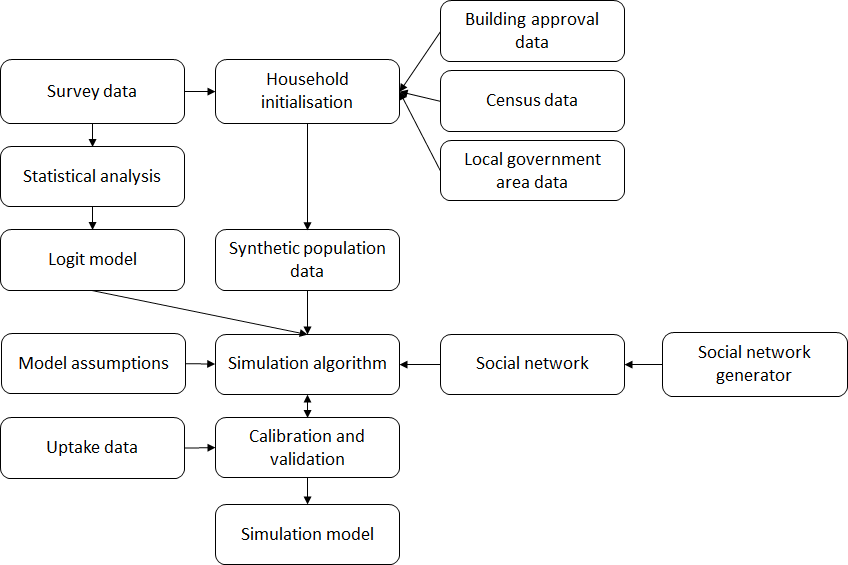
To evaluate the Logit model for aggregate level prediction we compared the predicted historical solar PV uptake levels (based on the logit model) with historical uptake levels. This identified two concerns that the ABM framework could address:
- There is a higher than expected adoption rate of solar PV systems in areas where many new dwellings have been built. This indicates a window of opportunity, i.e. when people build a new house, many will install solar panels at the same time or within a year or two. When we discussed this issue with experts who have tracked the adoption of solar PV systems in Australia, they confirmed that this pattern of behaviour has been commonly observed.
- In areas of higher than expected adoption rate, we undertook visual inspection in Google Maps to gain a greater understanding. We found that solar panels often appear in clusters, especially when they can be seen from the street – something that has been discussed in several other articles (Bollinger & Gillingham 2012; Copiello 2018). For example Parkins et al. (2018) have shown that the visibility of solar PV systems has a strong effect on the intention to purchase. This indicates a contagion effect that could potentially be described by spatially described social networks.
Data and statistical analysis
We adopt the critical realist standpoint that theories contribute a limited but incomplete set of useful insights, which is also in line with Mixed Methods thinking (Mukumbang 2021). According to this way of thinking, fuller perspectives on complex social and economic phenomena require insights from multiple theories. Therefore, we first consider any factors that have been successfully used in previous modelling efforts in predicting solar PV adoption behaviour. This also acknowledges that there is a need to consider the context and that we always need to consider psychological, demographic, economic and physical conditions and contexts alike.
We identify factors that influence solar PV adoption behaviours, as shown in Table 1, based on a brief review, and we note that this set of factors overlaps largely with the systematic review of predictors of residential solar PV adoption undertaken by Alipour et al. (2020).
To further identify predictors of solar PV adoption behaviour, beyond those reported in in academic literature, we also sought inputs from experts at the CSIRO (where several of the authors were employed at the time of study), via peer-to-peer conversations. CSIRO is Australia’s National Science Agency, who have been collecting data on attitudes and beliefs relating to solar PV adoption over several years.
The list of predictors in Table 1 is largely consistent with different theories, including Theory of Planned Behaviour that describes the importance of beliefs and self-efficacy in influencing behaviour (Ajzen 1991), theories about how people are influenced by the presentation of information when making choices (Frederiks et al. 2015; Jager & Janssen 2012; Kahneman & Tversky 2000), theories about the importance of aesthetics and personal taste in shaping decisions (Rosenberg 2011), and theories about how attitudes towards novelty and innovation influences choices (Rogers 2003).
| Category of predictor | List of predictors | References, if any, exploring the role of the predictor(s) on uptake |
|---|---|---|
| Demographic | Gender, age, household income, education, household ownership, household size, etc. | Alipour et al. (2020), Copiello et al. (2018), Dong et al. (2017), Lee & Hong (2019), Batista da Silva et al. (2020), Moglia et al. (2017) |
| Location and characteristics of the home | Place of residence, type of dwelling, size of the dwelling, tenure category (i.e., own outright vs mortgage vs renting etc), solar radiation, latitude and altitude. | Alipour et al. (2020), Copiello et al. (2018), Dong et al. (2017), Ford et al. (2017), Lee & Hong (2019), Moglia et al. (2017), Batista da Silva et al. (2020), Busic-Sontic & Fuerst (2018) |
| Social influences | Peer adoption of solar PV systems, media, information from government, promotions by suppliers, visual cues of solar PVs in the neighbourhood, word of mouth, etc are linked with higher rates of adoption in a neighbourhood. | Alipour et al. (2020), Dong et al. (2017), Ford et al. (2017), Lee & Hong (2019), Moglia et al. (2017), Stavrakas et al. (2019), Bollinger & Gillingham (2012), Busic-Sontic & Fuerst (2018) |
| Financial | Disposable income, access to funds to pay for systems, the upfront cost of systems, financial incentives, payback period. | Agnew et al. (2018), Alipour et al. (2020), Batista da Silva et al. (2020), Busic-Sontic & Fuerst (2018) Copiello (2018), Dong et al. (2017) Ford et al. (2017), Lee & Hong (2019) Moglia et al. (2017), Stavrakas et al. (2019) |
| Environmental beliefs and concerns | Concern about environmental issues, the belief that the environment is under threat. | Agnew et al. (2018), Alipour et al. (2020), Moglia et al. (2017) |
| Beliefs about solar PV systems | Beliefs about solar PV systems to variously help the environment, increase or decrease the market price of electricity, being a good financial investment, being something that households are capable of managing; being visually unappealing, being expensive or cheap, helping to reduce electricity bills, increase the value of real estate, help support self-sufficiency, etc. | Alipour et al. (2020), Ford et al. (2017), Moglia et al. (2017), Stavrakas et al. (2019) |
| Individual priorities | Self-sufficiency, having a (thermally) comfortable home, climate change mitigation, having the latest technology, being frugal, etc. | Agnew et al. (2018), Alipour et al. (2020), Ford et al. (2017), Moglia et al. (2017) |
| Personality and knowledge of systems | Agreeableness, conscientiousness, neuroticism, openness to experience, understanding of systems- | Busic-Sontic & Fuerst (2018), Ford et al. (2017) |
| Construction of new homes | It is argued by experts that households are more likely to install solar PV systems within a year or two after they build a new home. | Key informants i.e., researchers on the topic of sustainable homes, and new construction in Australia |
Survey data
Informed by Table 1, data on householder views, behaviours and attitudes relating to solar PVs were collected using an email-based survey using SurveyMonkey software by the accredited survey panel company, The Online Research Unit (Theoru 2021), between 23rd June and the 7th July 2019. We used quotas on education, gender and age to replicate distributions like those in the Australian Bureau of Statistics census (Australian Bureau of Statistics 2016). Participants that passed quota limitations and geographical and age-based screening were recruited from an online panel. The survey questions are available in the appendix. The size of the sample was 1,042 with all respondents residing in the Melbourne Metropolitan Region. The survey explored 132 questions. The average completion rate amongst participants was 64% and the average time spent on the survey was 13 minutes. The survey was consistent with CSIRO’s Ethical Conduct in Human Research Policy and received ethics clearance (#081/19).
In the sample, 23% of respondents reported owning a solar PV system, and a further 15% noted an intention to purchase in the next 6 months, with 63% noting that they neither own nor intend to purchase such a system. In comparison, at the time of the survey, only 14% of households across Melbourne metropolitan region owned solar PV systems, indicating a selection bias towards those with solar PV systems.
Acknowledging that the sample is biased towards those more likely to adopt solar PV systems, we adjust for this in the model, both by adopting weighted estimates, adjustment factors (see Section 4.1 on the calibration), as well as through the way that agents are initialised to represent known distributions of socio-economic attributes.
There were 48% male and 51% female respondents, with 1% either no response or other gender. 9% of respondents were in the age group 18-24, 20% were 25-34, 18% were 35-44, 17% were 45-54, 15% were 55-64, 12% were 65-74 and 8% were 75 and older. This shows an acceptable distribution of gender and age groups.
We note some sampling bias towards higher education i.e., 12% had a postgraduate qualification, 24% had an undergraduate degree (compared with 22% of the general population who have an undergraduate or postgraduate degree) but only 0.5% of the respondents had primary school education as their highest level of attainment (compared with 9% in the general population). For estimates of propensities in the general population, the 2016 census is referred to Australian Bureau of Statistics (2016).
Apart from the survey data, we also use census data from the Australian Bureau of Statistics (Australian Bureau of Statistics 2016); spatially (per postcode) and temporally (per month) granular adoption data from the Clean Energy Regulator (Clean Energy Regulator 2020); as well as data on building approvals from local councils (.idcommunity 2020).
Belief constructs
Key predictors of behaviour are known to be beliefs and attitudes. Therefore, the survey measured participants’ beliefs about solar PV systems based on their responded level of agreement with the statements shown in the first column of Table 2, A Likert scale of Strongly disagree (0), Disagree (0.25), Neither disagree nor agree (0.5), Agree (0.75), and Strongly agree (1) was used. Average scores were calculated by assigning numerical values corresponding to the responses as per numbers in brackets. Average scores are shown in Table 2, and the correlation between such beliefs and the ownership or stated intention to purchase a solar PV system. Table 2 shows the average scores of these beliefs. We also note that the correlation between perceptions and the self-reported ownership or stated intention was statistically significant in many cases.
| Beliefs about Solar PV panels | Average score Pearson correlation with ownership; with p-value and significance level | Pearson correlation with stated intention to purchase; with p-value and significance level | ||
|---|---|---|---|---|
| Solar PV panels are good for the environment# | 0.76 | 0.04 (0.1)** | 0.04 (0.1) ** | |
| Solar PV panels have a high upfront cost \(\wedge\) | 0.70 | -0.12 (0.0001)*** | -0.12 (0.0001)*** | |
| Solar PV panels help reduce electricity bills# | 0.70 | 0.08 (0.005)*** | 0.09 (0.002)** | |
| Installing PV panels is an ethical thing to do# | 0.68 | 0.15 (<.0001)*** | 0.19 (<.0001)*** | |
| Solar PV panels are a good financial investment# | 0.66 | 0.15 (<.0001)*** | 0.23 (<.0001)*** | |
| Solar PV panels will increase the value of my property# | 0.65 | 0.17 (<.0001)*** | 0.11 (0.0002)*** | |
| Solar PV panels help reduce power outages# | 0.59 | -0.06 (0.03)** | 0.01 (0.4) | |
| Solar PV panels enable households to become independent from the grid# | 0.58 | -0.01 (0.4) | 0.07 (0.012)** | |
| Installing PV panels decreases electricity prices for everyone# | 0.56 | 0.04 (0.1)* | 0.14 (<.0001)*** | |
| Installing PV panels increases electricity prices for everyone \(\wedge\) | 0.49 | -0.05 (0.05)** | 0 (0.5) | |
| Solar PV panels look ugly \(\wedge\) | 0.48 | -0.15 (<.0001)*** | -0.09 (0.002)** | |
| My property is not suitable for installing solar PV panels (shade, inadequate roof orientation etc)& | 0.42 | -0.21 (<.0001)*** | -0.16 (<.0001)*** | |
| Solar PV panels are not permitted or suitable in my area (i.e., body corporate restrictions) | 0.38 | -0.27 (<.0001)*** | -0.24 (<.0001)*** | |
| Solar PV panels is mainly about showing off \(\wedge\) | 0.32 | -0.13 (<.0001)*** | -0.05 (0.05)** | |
To enable logistic regression modelling, we had to deal with the issue of multicollinearity in beliefs. In other words, we found that someone who thinks that solar PV systems are mainly about showing off is also more likely to think that they are ugly. Therefore, we created latent constructs that are more suitable for use in regression modelling, and identified three variables:
- Solar PV systems are good: explained by variables indicated by # in Table 2;
- Solar PV systems are bad: explained by variables indicated by \(\wedge\) in Table 2;
- Solar PV systems are inappropriate where I live: explained by variables indicated by & in Table 2
Interestingly, we identified these three beliefs based on Factor Analysis where positive and negative beliefs seemingly should be two sides of a spectrum, but we found they are not. In fact, the belief that solar PVs are good (a construct of several beliefs), and the belief that solar PVs are bad (a construct of another set of beliefs) are uncorrelated. In other words, the same person could simultaneously hold beliefs that solar PVs are good, and that solar PVs are bad.
These beliefs do influence the decision to adopt solar PV systems. Among the participants who had on balance a more positive view of solar PV systems, 25% had already adopted these systems. Among those who were on balance neutral, 20% were adopters. Among those with a negative view of solar PV systems, only 5% reported ownership.
Furthermore, dwelling type influences whether respondents report that there is space for solar PV systems at their property (house: 80%, detached dwelling: 61%, other: 73%, apartment: 31%). Rates of solar PV ownership for those with self-reported space for a system is 30%, compared to 9% for those who report that they do not have space (presumably for an additional system). Tenure type influences the chances of solar PV ownership (own home outright: 31%, own with a mortgage: 25%, rent: 7%).
Logit regression
To explore the relative importance of factors outlined in the survey in terms of their influence on ownership of solar PV systems or a stated intention to purchase such as system, we undertook logistic regression (logit) analysis. With two different binary dependent variables (\(Y_{1}=1\) if own and \(Y_{2}=1\) if intent to own, and 0=non-adopter), a Binomial logit model was used where the logistic regression function to describe the probability of adoption or intent to purchase a solar PV system is based on the following equation:
| \[ P_{i}(own \; or\; intent) = \frac{1}{1 + \exp (\beta_{0} + \beta_{1}x_{1} + \beta_{2}x_{2} + \dots \beta_{n}x_{n})}\] | \[(1)\] |
In Equation 1, there are different variables for ownership versus stated intent to purchase solar PV systems (as described in Table 3 and Table 4). \(X_{i}\) refers to the independent variable \(i\), and \(\beta\)-parameters refer to the respective coefficient.
The model was developed based on stepwise regression and backward elimination i.e., starting with all candidate variables, and successively removing those found to be least statistically significant, until all remaining independent variables are shown to have a statistically significant influence on the adoption rate. The resulting model is shown in Table 3 and Table 4, with \(\beta\)-parameters shown in the “estimate” column (the intercept is \(\beta_{0}\)), and the significance test value (\(Pr(> \lvert z \rvert)\)) which is used to establish the significance level of the independent variable in the resulting model. Most of the independent variables are self-explanatory, but the variable “good access” is a composite measure of self-reported access to shops, schools, health care services, recreation facilities, open space, public transport, jobs and affordable housing in the area that the respondent lives.
| Coefficients (\(x_{1 \dots i}\)) | Estimate (\(\beta\)) | p-value | Significance level |
|---|---|---|---|
| Intercept | -2.81 | 0.006 | ** |
| Dwelling-type: Apartment | 0 | N/A | N/A |
| Dwelling-type: Detached | 1.35 | 0.02 | |
| Dwelling-type: House | 1.25 | 0.02 | |
| Dwelling-type: Other | 2.67 | 0.003 | ** |
| Factor(Tenure): Mortgage | 0 | N/A | N/A |
| factor(Tenure): Other | -0.25 | 0.5 | |
| factor(Tenure): Own | 0.25 | 0.2 | |
| factor(Tenure): Rent | -1.18 | 0.0002 | *** |
| Belief that solar PVs have a high upfront cost | -1.85 | 5.4E-06 | *** |
| Number of bedrooms | 0.39 | 0.0009 | *** |
| Enough space for solar PVs: No | 0 | N/A | N/A |
| Enough space for solar PVs: Unsure | -1.11 | 0.04 | |
| Enough space for solar PVs: Yes | 0.57 | 0.10 | . |
| Belief that solar PVs are good | 0.54 | 0.54 | |
| Belief that solar are bad | -5.0 | 0.004 | ** |
| Property not suitable for installing solar PVs | -2.09 | 0.0007 | *** |
| Prioritising have a thermally comfortable home | 1.48 | 0.003 | ** |
| Self-reported good access to services in the area | -2.43 | 3.6E-05 | *** |
| Observations | |||
| Pseudo \(r^{2}\) | |||
| Coefficients (\(x_{1 \dots i}\)) | Estimate (\(\beta\)) | p-value | Significance level |
|---|---|---|---|
| Intercept | -1.54 | 0.074 | . |
| Dwelling-type: Apartment | 0 | N/A | N/A |
| Dwelling-type: Detached | 0.24 | 0.48 | |
| Dwelling-type: House | -0.09 | 0.78 | |
| Dwelling-type: Other | 0.79 | 0.31 | |
| Tenure: Mortgage | 0 | N/A | N/A |
| Tenure: Other | -1.26 | 0.0009 | *** |
| Tenure: Own | -0.13 | 0.49 | |
| Tenure: Rent | -1.50 | 6.2E-10 | *** |
| The belief that solar PVs have a high upfront cost | -1.94 | 1.8E-07 | *** |
| Number of bedrooms | 0.30 | 0.004 | ** |
| Enough space for solar PVs: No | 0 | N/A | N/A |
| Enough space for solar PVs: Unsure | -0.35 | 0.32 | |
| Enough space for solar PVs: Yes | 0.88 | 0.00096 | *** |
| Belief that solar PVs are good | 2.3 | 0.0055 | ** |
| Belief that solar PVs are bad | -2.66 | 0.080 | . |
| Property not suitable for installing solar PVs | -1.84 | 0.0005 | *** |
| Prioritising have a thermally comfortable home | 1.51 | 0.0007 | *** |
| Self-reported good access to services in the area | -2.48 | 3.1E-06 | *** |
| Funds available for emergency expense | 0.67 | 0.0065 | ** |
| Household Income High | 0 | N/A | N/A |
| Household Income Low | -0.088 | 0.71 | |
| Household Income Medium | -0.167 | 0.42 | |
| Belief that PVs are good * Belief that PVs are bad | 4.86 | 0.013 | |
| Observations | |||
| Pseudo \(r^{2}\) | |||
Simulation framework
The purpose of our model is to provide aggregate level predictive analysis of solar PV adoption across a metropolitan region, as a foundation for a model that can help provide useful information for decision-makers and infrastructure planners. The survey data, as well as the logit model was embedded into a hybrid ABM. This hybrid model is similar to that which was previously described by Lee & Hong (2019) in that the core engine is a Logit model, around which a micro-simulation model has been wrapped, allowing for describing the heterogeneity of the population as well as the influence of the key opportunity for solar PV installation associated with new construction of a house as well as the peer-influence on decisions. We describe the model using a commonly used protocol for describing ABMs, the Overview, Design concepts and Details protocol (Grimm et al. 2010), with descriptions provided in Appendix A. Calibrated model parameters are shown in Table 5, Table 6 and Figure 3.
Social network: As there is no social network data available, households are connected in a social network according to a theoretically constructed Barabasi-Albert graph (a scale-free network). This is an algorithm that generates a random scale-free networks using a preferential attachment mechanism, which has been sometimes considered when developing ABMs (Sabzian et al. 2020; Sznajd-Weron et al. 2014; Wang & Collins 2015). Further description of the social network type is provided by Barabási & Albert (1999).
Scale: The model is being applied at numerous local government areas within which synthetic populations are generated based on existing demographic data from the Australian Bureau of Statistics and local government resources (Australian Bureau of Statistics 2016;.idcommunity 2020).
Initialisation: Households are generated at the start of the simulation period representing the known population size, and number of households at that time. The representativeness of attribute assignment similar to that used by Moglia et al. (2017) where assignment is based on individual responses. Representativeness therefore relies on having enough responses (approximately >30) in each combination of key attributes, which we do. To represent housing growth i.e., construction, new households are generated in each yearly timestep, based on building approval data.
Heterogeneity: All household attributes are assigned so that distributions, correlations and conditional probabilities are consistent both with the household survey as well attribute distributions as per the Australian Bureau of Statistics community profiles for each local government area based on the 2016 census data (Australian Bureau of Statistics 2016) and community profiles from the profileid website (.idcommunity 2020).
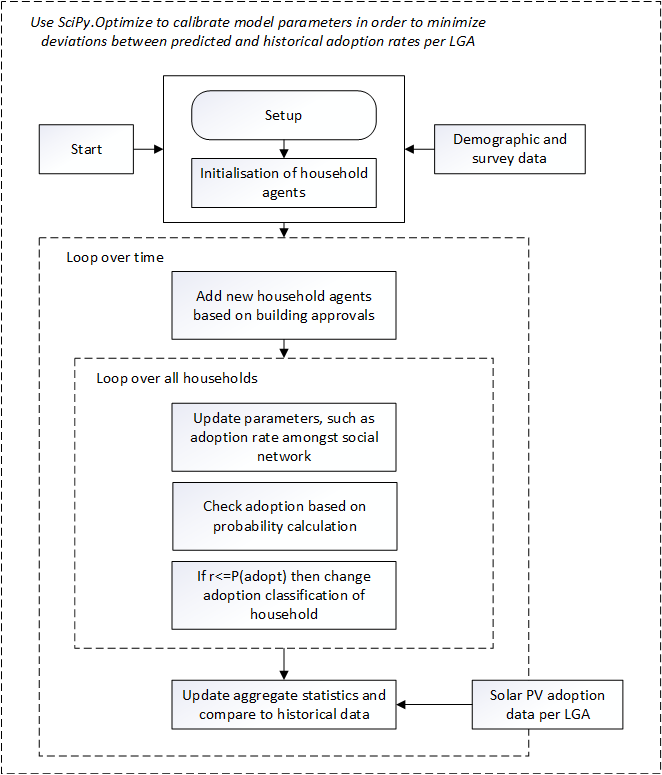
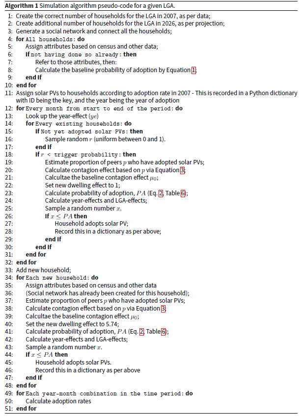
Simulation process: the process overview and schedule are illustrated in the diagram in Figure 4 showing the sequence of steps in the simulation. The simulation process is also described in pseudo-code in Algorithm 1. From a household perspective, the adoption of solar PVs is a two-step process, i.e. first the household needs to reach a decision point where the chance of adoption is based on household attributes etc, and the second, the outcome of that decision is to adopt solar PVs (with the probability of this decision described by Equation 2). Within the simulation schedule, the household adoption probability is calculated using these equations and parameter values in Table 5:
| \[ P(Y_{i,j,k} = 1 \lvert Y_{i, j-1, k} = 0) = \frac{\omega \delta_{t} \gamma_{i} \theta_{k,t} \mu_{k,j} r_{j}}{1 + \exp (\beta_{0} + \beta_{1}x_{1} + \beta_{2}x_{2} + \dots \beta_{n}x_{n})}\] | \[(2)\] |
| \[ \mu_{k,t} = 1 + \mu_{0} \overline{Y_{k,t}}\] | \[(3)\] |
| \[ E(Y_{i,j,k}) = \frac{\delta_{t} \gamma_{i} \theta_{k,t} \mu_{k,t}}{1 + \exp (\beta_{0} + \beta_{1}x_{1} + \beta_{2}x_{2} + \dots \beta_{n}x_{n})} \sum_{t = 2007}^{j} (1 + \mu_{0} \overline{Y_{k,t}}) P(Y_{i, t-1, k} = 0)\] | \[(4)\] |
Here, \(Y_{I,j,k}\) is the stochastic variable describing whether agent \(k\), within LGA \(I\) and in year \(j\), have adopted solar PVs. \(\beta\) model parameters are described in Table 5. Importantly, each household has a probability of “making a choice” each time step (2.3% chance each month as per Table 5) – whilst those that build a new home definitely (100%) make a choice. At this time, once making a choice whether to install solar PVs, the probability of choosing to install is described by Equation 2. \(\omega\) is a generic adjustment effect that is calibrated. \(\delta_{t}\) is the year-effect factor describing the different policy settings and temporal contexts for each year, \(\gamma_{i}\) is a spatial effect describing the differences between local government areas (LGAs) not otherwise explained in the demographics and housing stock. \(\mu_{k,j}\) is the new dwelling effect for agent \(k\) in year \(j\). \(r_{j}\) is the rebate factor applied in year 2019, and in 2020. The new dwelling effect is one except in the year that a building is being constructed. Equation 4 shows the statistical expectation value for the variable \(Y\).
Contagion effect: The contagion effect \(\mu_{k,j}\) is calculated using Equation 3, where \(\overline{Y_{k,t}}\) is the average adoption rate of solar PV systems within the connected nodes in the household \(k\)’s social network at year \(t\). As per Kiesling et al. (2012) this is a meso-level social influence commonly used in innovation diffusion models that signifies group conformism, and social comparison; in line with how to model the role of social influence via subjective norms in the Theory of Planned Behaviour (Zhang & Vorobeychik 2019) which relatively closely aligns with our model.
Modelling Results
Here we report on the modelling results, including calibration of parameters, simulation in several LGAs for several years, as well as exploration of the model’s predictive capacity.
Calibration
Parameters were calibrated by minimising the square sums of the deviation between observed and simulated adoption rates for the period 2008-2019 aggregated for all the LGAs (i.e., a version of the Method of Least Squares). The optimisation was enabled by the Python scipy.optimize module. The calibration occurred by systematically varying parameter values and selecting the ones that help reduce the aggregate errors across several thousand of simulations.
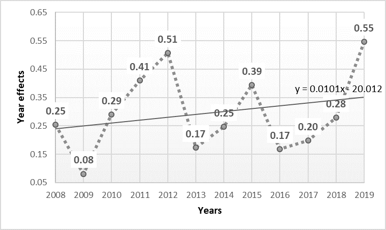
To account for the higher rates of adoption in the survey population compared to the broader population, we use the adjFactor as shown in Table 5 and Equation 2. Calibrated key parameters in the simulation that drives the dynamics are shown in Table 5. For temporal variability, we calibrated a series of Year-Effects (shown in Figure 3). To describe spatial variability, we calibrated a series of LGA-effects, to capture differences in areas, in terms of their contextual suitability for adoption of residential solar PV systems, and these are shown in Table 6.
Finally, in terms of calibration, we found later that for the initial forward-validation year (2020) the estimated R-Squared was first as low as 0.66, however further investigation of spatial differences arising in 2019 meant that we explored the results of a solar PV rebate policy introduced in 2019 by the Victorian State government. This rebate was available for households below an income threshold (AUS$180,000 per year income), and for homes below a certain value. Not surprising therefore, the spatial variation in 2019 and 2020 had a correlation of 0.6 with an estimate of the proportion of households who are eligible in the LGA, and a correlation of 0.69 with average monthly household mortgage repayments. Based on this, we introduced an LGA-based adjustment factor for year 2019 and 20201 with the adjustment-factors applied in those years shown in Table 6.
| Parameter | Description | Value |
|---|---|---|
| Adjustment factor (\(\omega\)) | Accounting for differences in adoption in survey population vs general population. | 0.61 |
| Baseline contagion effect (\(\mu_{0}\)) | Describing how the chance of adoption increases with adoption within a social network, as per Equation 3. | 6.32 |
| New dwelling effect (\(\mu_{k,j}\)) | Describing the increased chance of adoption within the year that a new dwelling is constructed. | 5.74 |
| The baseline trigger rate (\(f\))- a frequency | Recognising that everyone does not decide whether to adopt solar PVs every month, there is a baseline chance of making a decision. | 0.023 (2.3%) |
| Local government area | Calibrated LGA-factor value | Rebate factor (2019-2020) |
|---|---|---|
| Casey | 1.01 | 1.12 |
| Frankston | 0.81 | 1.22 |
| Wyndham | 0.79 | 1.07 |
| Hume | 0.76 | 1.20 |
| Melton | 0.69 | 1.14 |
| Whittlesea | 0.59 | 0.89 |
| Knox | 0.86 | 0.91 |
| Kingston | 0.71 | 0.86 |
| Monash | 0.68 | 0.93 |
| Moreland | 0.57 | 0.44 |
| Glen Eira | 0.49 | 0.64 |
Simulation
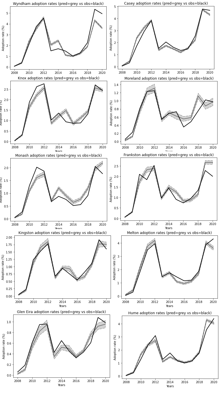
Using the calibrated as well statistically estimated parameters, the result from 100 simulations in each LGA are illustrated in Figure 4. The average simulated adoption rate (i.e., the percentage of households in an LGA that invest in solar PV systems in that particular year) over 100 simulations (with bands showing the 95 % confidence interval) is shown in grey and the observed adoption rates, based on data from the Clean Energy Regulator (2020), is shown in black. The simulation model predicts adoption rates that are largely within the bands of what was observed over these years, but we note that the year 2020 was problematic in terms of a validation dataset due to the recent introduction of widely available government rebates to support purchases of new residential systems. We therefore adjusted for this effect in the year 2020.
Sensitivity
As per Equation 4, several parameters increase or decrease the average adoption rates in a linear manner i.e., this refers to2:
- The adjustment factor (\(\omega\)), the baseline contagion effect, \(\mu_{0}\), and the baseline trigger rate (\(f\)).
- The new dwelling effect \(\mu_{k,j}\) increases adoption rates linearly in relation to rates of new housing construction.
- A higher contagion effect \(\mu_{k,t}\) increases adoption in the later years over and above what would otherwise be expected. A positive feedback effect is based on an autoregressive element, which is relatively small compared to other effects.
We don’t report on sensitivity analysis of key parameters as this would provide only trivial insights (i.e., a 10% increase in the parameter value would create a 10% impact on results etc).
Predictive capacity
We evaluate the modelling suite’s capacity to predict both at the micro-level and macro-level against both survey and independent data, in line with recommendations by Zhang & Vorobeychik (2019). We also note also that we do not have a very large number of parameters that we have calibrated, and errors are similar for the test data sets as they are for the training dataset, and therefore it seems likely that we have avoided over-fitting.
Micro-level predictive validation
To evaluate this model’s capacity to predict whether an individual household has already installed a solar PV system, we explored the Binomial logit model, against survey participant responses using a confusion matrix (see Table 4). A confusion matrix describes the predictive performance of Equation 1 by summarising the number of correctly and incorrectly predicted solar PV adopters and non-adopters. The overall predictive accuracy of Equation 1 is 79%, although non-adoption is predicted more accurately than adoption. This issue is unsurprising because other determinants trigger a household’s choice to install solar PVs beyond, such as opportunity, practice, social influence and contextual or emotional factors present at a moment in time, but which are difficult to capture in a survey. It should be noted that the intention is not to accurately predict individual behaviour, but instead to estimate aggregate behaviours which the model does well.
Based on Table 7, we can calculate the:
- Accuracy – percentage of predictions that are accurate: 79%
- Precision – ability to accurately predict adoption: 60%
- Sensitivity – proportion of adopters correctly predicted: 26%
In other words, a relatively high accuracy, but a relatively lower sensitivity. It is notable that micro-level validation reporting was not found in the reporting of similar models.
| \(N=1040\) | Predicted non-adopter | Predicted adopter |
|---|---|---|
| Actual non-adopter | 762 | 41 |
| Actual adopter | 175 | 62 |
Macro-level forward validation
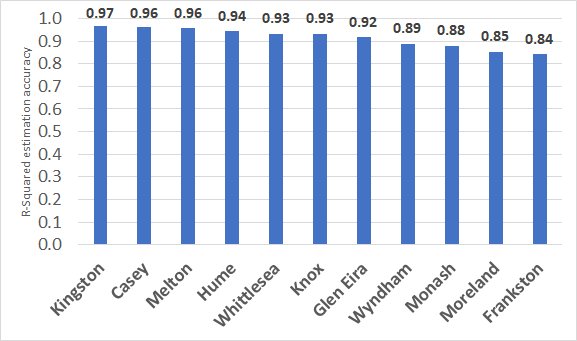
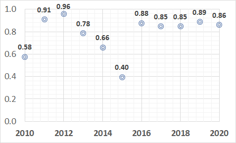
Aligned with suggestions by Zhang & Vorobeychik (2019) we have calibrated the model parameters based on data from 2010-2019 and validated the model based on data during 2020 (i.e., forward validation). To evaluate the macro-level predictive capacity, we calculate the R-Squared (as traditionally defined: 1 minus the unexplained variance divided by the total variance) for each of the LGAs and each of the years. The total variance is the statistical variance of all observations, while the unexplained variance is the statistical variance of the errors. The R-Squared results are shown in Figure 5 and Figure 6, representing the results from the full calibration period. Spatially, the R-Squared ranges from 0.62-0.97 with only Glen Eira and Moreland having values below 0.85. Temporally, the predictive capacity ranges from 0.40-0.96. For the validation year in 2020 (i.e., the forward data), the R-Squared was first 0.66, indicating a reasonable goodness-of-fit which can nonetheless be improved. After deliberation, it was deemed that the major difficulty was the introduction of a new rebate for households with certain eligibility criteria that limited uptake. After calibrating a rebate effect (see Calibration Section, 4.1) the R-Squared was 0.86. Although there is variation spatially and temporally in predictive capacity, the aggregate predictive capacity is relatively high across either dimension. Unfortunately, similar models are not reporting R-Squared (which we think is the appropriate measure here) for their approaches, so it is difficult to compare (Lee & Hong 2019; Zhao et al. 2011).
Discussion
The analysis undertaken in this paper raises important questions and implications. In our discussion, we focus on the following insights and topics:
- The importance of perceptions and attitudes for solar PV adoption.
- The temporal variability in adoption rates, and the likely causes of this.
- The spatial variability in adoption rates, and the likely causes of this.
- Housing construction as a key driver of adoption, and its intersection with housing tenure i.e., renters are much less likely to have solar PV systems.
- The opportunities for data to improve accuracy and predictive modelling.
- Who are the likely end-users of the model?
- What is the overall value-add of using an ABM framework?
Perceptions of solar PV systems
When beliefs about solar PV systems were analysed using confirmatory factor analysis, three latent variables were identified: “solar PVs are good”, “solar PVs are bad”, and “solar PVs are not suitable where I live”, that influence the decision to install solar PV systems. This indicates that someone who has positive views about solar PVs in one respect is also likely to have positive views about solar PVs in another way; and vice versa.
This polarisation of beliefs gives the impression of affective response to solar PVs i.e., the mention of these systems – as a stimulus – generates either a broadly positive or negative response. This indicates that the beliefs may be largely driven by emotion – and therefore may be less enduring than thought and could potentially instead be referred to as perceptions. This is similar to what is described in the article by Ransan-Cooper et al. (2020) concerning solar PVs and home battery systems.
This emotive response to solar PVs is perhaps not surprising given the political context of Australia where action on climate change has been highly politicized, with a deep political divide on the need for climate change action (Kousser & Tranter 2018). Experiments by Kousser & Tranter (2018) has shown that individuals in Australia tended to change their positions on renewable energy and climate change mitigation when learning about the positions of political leaders that they supported. This also aligns with the observation around temporal variability in adoption rates that have seemingly a three-year cyclic pattern with the lowest rates of adoption reasonably well aligning with federal elections in Australia. However, this evidence is so far circumstantial and can’t be statistically confirmed, especially, as key changes in feed-in tariffs and rebate policies have changed at similar times.
On temporal variability
Our model does not yet, except for in relation to the rebate available to households in 2019-2020, capture financial incentives, and we know that there were two types of financial incentives in the period 2005-2020. Firstly, a feed-in tariff where householders are paid for excess electricity that is supplied into the grid. For a period from 2009-2011 this was 60 cents/kWh and then dropped down to 25 cents/kWh until 2015, when it dropped briefly to 5 cents/kWh. Since then, the feed-in tariff has been in the range of 7 cents per kWh and 12 cents per kWh which is the current setting. Thirdly, a rebate, where the state and/or federal government pays part of the purchase cost; generally subject to an income test and a house price test.
Drawing on these insights, we are exploring the causal mechanisms behind the year-effect, and indications from a study by Currie et al. (2019) are that this is best explained by taking into account rebate size, feed-in tariffs, the average price of a new system, electricity price, as well as business confidence. This aligns with what we are seeing in the data, although we do not have enough data points to confirm this here.
It is also notable that federal elections, where action on climate change was a highly contested topic, occurred in 2010, 2013, 2016 and 2019; which except for 2019 is relatively closely aligning with strong dips in adoption rates. This is likely not coincidental.
We also found in our model that the incorporation of a social network effect, contributed to a description of why the adoption of solar PVs accelerates over time, something which has been observed in practice.
On spatial variability
To give an insight into what drives the spatial variability, we explored correlations and found at least three variables with non-trivial correlations with the LGA-factor, and these are shown in Table 3.
| LGA | Category of area | Average size (kW) of solar installs 2001-2020 | Public open space as % of the total area | % of construction that are new buildings |
| Casey | Outer suburb | 4.59 | 10% | 77% |
| Frankston | Outer suburb | 4.40 | 9% | 46% |
| Wyndham | Outer suburb | 5.06 | 6% | 84% |
| Hume | Outer suburb | 5.38 | 9% | 78% |
| Melton | Outer suburb | 4.58 | 5% | 41% |
| Whittlesea | Outer suburb | 4.82 | 8% | 59% |
| Knox | Middle suburb | 4.50 | 13% | 37% |
| Kingston | Middle suburb | 5.10 | 13% | 38% |
| Monash | Middle suburb | 4.47 | 9% | 39% |
| Moreland | Inner suburb | 4.34 | 10% | 32% |
| Glen Eira | Inner suburb | 4.34 | 4% | 40% |
The average size of solar PV systems installed (2001-2020) has a correlation (with the LGA-factor) of 0.18; the proportion of space being public open space has a correlation (with the LGA-factor) of 0.45, and the proportion of new construction that are new homes has a correlation (with the LGA-factor) of 0.55. This points towards the unexplained variability being primarily about the availability of space for solar PV systems, as well as towards the need for more accurate data for new homes rather than new home constructions in the simulation model. Future models should account for this effect.
A regression model with these variables to describe the LGA-factor has an R-squared of 0.72 although the average size of the solar PV system had a non-significant contribution. Further spatial analysis is underway to understand the reason for the remaining 28% of the spatial variability. This variability may be linked with spatial variation in dwelling types, urban form and building shadow, tenure and natural characteristics of areas (e.g., foliage, elevation) which may impact on the productivity of small-scale rooftop solar PV systems.
A range of local circumstances are known to influence spatial variability. For example, in outer suburban areas there can be relatively lower adoption due to extensive industrial or parkland areas, or university precincts. In more densely built-up areas or areas with larger proportions of rental properties, property rights dimensions (such as body corporate restrictions, air-rights, common space, ownership of usable surfaces) as well as coordination barriers (i.e., decisions may need coordination of multiple users and owners to maximise efficiency of microgrids rather than individual rooftop solar PV systems) may inhibit the uptake of rooftop solar PV systems.
Housing construction as a catalyst of solar PV adoption
A key finding in this article is how construction of new housing, at the very least in the context of Melbourne metropolitan region, is a key driver of solar PV adoption. To show this effect, we have drawn on building approval data and this contributes significantly to the accuracy of predictions. Alipour et al. (2021) noted that this type of data, on construction, was previously only incorporated in one other study on this topic, and never within a comprehensive framework such as the one described here.
In this article, we have described the adoption of solar PVs on newly constructed homes in a relatively crude way based on: 1) the notion that construction triggers a decision whether to install solar PVs, due to the opportunity that has arisen, and 2) that the likelihood of adoption is a factor \(\mu_{k,j}\) (here calibrated to 5.74) larger than in other circumstances for the same household. With the available data, only such a relatively crude model is feasible, which is to some extent regrettable.
This lack of appropriate data that connects solar PV adoption with new home construction shows a key knowledge gap. Importantly, when we designed the survey, the role of construction was not considered. This is because the role of housing construction in driving solar PV adoption was not widely acknowledged in literature (if at all), and that we only learnt about this effect after interrogation and validating the model, which led us to make adjustments, which was also confirmed by solar PV experts that we conferred with about this result. In other words, we propose that further research undertaken so that:
- Data is collected specifically on solar PV adoption for new homes. Experts argue that there is a window of about 2 years after construction when there is an increased chance of adoption. Either because of the opportunities associated with construction, and secondly as experts report that households commonly find the energy efficiency of the new home to be lacking, and therefore commonly opt for installing solar PVs to compensate.
- Data is collected to better understand the socio-psychological and economic drivers for adoption of those who build new homes, or that retrofit existing homes.
Data improvement for energy transition
The 79% accuracy of the predictions of ownership or intentions at an individual level could be improved. This indicates opportunities for gathering further data, and based on our analysis, there are areas of interests, specifically:
- Whether residents are living in recently constructed housing,
- Peer-influence,
- Awareness and access amongst participants relating to financial incentives, and
- Whether participants have been contacted by solar PV sales companies.
We also know that visual cues play a role in influencing adoption in some contexts (Bollinger & Gillingham 2012; Copiello 2018; Parkins et al. 2018). We propose that research is undertaken in Australia to confirm and quantify this effect, as well as to further build this into the quantitative approach.
Finally, there is an opportunity for more comprehensive modelling of the actor ecosystem. This more comprehensive approach for exploring the complexities of the residential Solar PV market in Australia could be enabled by incorporating the ecosystem of actors, providing a more integrated exploration of policies and interventions; for example, similar to that done by Moglia et al. (2018) when exploring residential energy-efficiency.
Potential users
We imagine two types of users of the model. Firstly, we imagine that this model could be usefully employed by electricity network planners, to inform infrastructure investment decisions. Secondly, we imagine that this model could be usefully employed by planners in government departments, whose job it is to fine-tune policies and regulations to boost the adoption rates of solar PV systems in a fair, equitable and cost-effective manner.
Therefore, our approach has been informed by discussions by energy distribution companies who require better predictive capacity for solar PV adoption, so that they can plan to have the required infrastructure. Among other things, this has informed our choice of spatial granularity (local government areas i.e., LGAs).
Conclusions
This paper reports on the development of a hybrid model to improve modelling and policy analysis for solar PV uptake. The modelling results show that high rates of adoption will likely accelerate into future years, but also that structural barriers can vary across the cities.
Methodologically, our study contributes to an emerging understanding of so-called hybrid approaches that integrate statistical methods within an ABM simulation framework. This combines the flexibility and exploratory capabilities of ABM with the empirical rigor of statistical methods. Our approach, as one instance of a hybrid approach, is shown to provide relatively accurate predictions at an aggregate level, but with clear directions of opportunities for improvements. The model also shows promising predictive capacity at a micro-level.
Methodologically, the hybrid approach provides a series of analytical advantages. First, greater flexibility for policy analysis. There is very considerable opportunity in an ABM to specify hypothetical scenarios without having to formulate such scenarios in terms of exact equations. Second, opportunity for calibration of parameters where appropriate statistical data is unavailable. In this article, we have included the proposed impacts of peer influence and construction of housing, even when statistical data is missing. Third, population heterogeneity. This allows for a richer understanding of how individual agents interact with each other and their environment. Fourth, model extensions are relatively straightforward, even when such extensions include non-linear and complex interactions. Extendibility is important because these types of models have the capacity act as knowledge representations, or knowledge artefacts that support ongoing learning.
In terms of the substantive contribution about modelling the adoption of residential solar PVs, the choice of predictors and collection of data on those predictors is the most important step for improving the accuracy of predictions. Despite reviewing a large body of literature on factors that influence solar PV adoption behaviour, and collecting data on those factors, we still seem to have missed some of the factors that focus on housing construction and peer influence. In fact, there seems to be no solar PV adoption model in existence that uses the full and comprehensive list of predictive factors. Our study represents one of the most comprehensive models in this respect.
We also note that to maximise predictive capacity unfortunately requires surveys of the community which comes at a cost. Modelling without such surveys may still provide somewhat accurate results, especially when it is possible to draw on accurate census data, solar PV adoption data and housing construction data. The most important dataset for enabling the hybrid approach is the solar PV adoption data provided by public agencies. This data proved very useful as it allows for calibration of model parameters. This data would be even more useful if there was a further breakdown of the characteristics of adopters, for example providing demographic or socio-economic data. We also note the role of policy settings, especially around financial incentives and this remains a topic that needs further exploration, although a key barrier in the current settings in Melbourne seems to relate to income and property value tests that exclude part of the population from access to rebates.
Furthermore, as perhaps the first study to do so, we have been able to demonstrate the role of housing construction in these adoption processes. Specifically, we have shown that, at the very least in the Melbourne context, housing construction is a critical mechanism by which uptake is accelerated, and conversely, we have identified that high rates of renting, and apartment living, or high rates of housing where local building regulations make adoption difficult, leads to significantly slower adoption. This shows the need for financial innovation and/or policy innovations and interventions that help overcome such barriers, as this would help to improve sustainability and equity outcomes.
As a next step, because we have embedded our modelling into an ABM framework, it is also possible/recommended to further explore the impact of more complex interventions in the market, for example, innovations that support renters or apartment dwellers to more easily adopt solar PV systems, or to provide more targeted interventions for those constructing new homes.
In summary, the comprehensiveness, design and details of this framework combined with a hybrid approach makes it a novel and useful contribution that can inform policy analysis as well as infrastructure planning decisions and support the transition towards greater uptake of renewable energy.
Data Availability Statement
The survey data for which this study is based are not publicly available due to privacy or ethical restrictions, although we may provide aggregate summaries of the data on request to the corresponding author. Other data is available via websites, as per references throughout.Acknowledgements
This study had some funding from the Low Carbon Living CRC. We also acknowledge productive contributions and discussions about solar PV adoption with Michael Ambrose, Elisha Frederiks, Stephen White and Luke Reedman from the CSIRO as well as James McGregor of BluetribeNotes
- An (OLS) linear regression model was used, resulting in the linear equation \(y_{adj} =0.4547 + 0.0215\; prop_{eligible} + 0.0006 \; amlr\). The model has an \(R^{2}\) of 0.68; \(y_{adj}\) is the rebate- specific adjustment factor applied in year 2019 and 2020; \(prop_{eligible}\) is the proportion of households which are below the income threshold for the rebate (i.e., eligible); and \(amlr\) is the average monthly loan repayments for households↩︎.
- It should be noted that whilst these effects are largely linear, there are added benefits of the simulation(ABM) framework which are further discussed later.↩︎.
References
AEMO, Australian Electricity Market Operator. (2021a). Generation information. Retrieved 17th February 2021 from: https://www.aemo.com.au/energy-systems/electricity/national-electricity-market-nem/nem-forecasting-and-planning/forecasting-and-planning-data/generation-information.
AEMO, Australian Electricity Market Operator. (2021b). NEM Data Dashboard. Retrieved 17th February 2021 from: .https://aemo.com.au/en/energy-systems/electricity/national-electricity-market-nem/data-nem/data-dashboard-nem.
AJZEN, I. (1991). The theory of planned behavior. Organizational Behavior and Human Decision Processes, 50(2), 179–211. [doi:10.1016/0749-5978(91)90020-t]
ALIPOUR, M., Salim, H., Stewart, R. A., & Sahin, O. (2020). Predictors, taxonomy of predictors, and correlations of predictors with the decision behaviour of residential solar photovoltaics adoption: A review. Renewable and Sustainable Energy Reviews, 123(109749). [doi:10.1016/j.rser.2020.109749]
ALIPOUR, M., Salim, H., Stewart, R. A., & Sahin, O. (2021). Residential solar photovoltaic adoption behaviour: End-to-end review of theories, methods and approaches. Renewable Energy, 170, 471–486. [doi:10.1016/j.renene.2021.01.128]
ALSHAHRANI, A., Omer, S., Su, Y., Mohamed, E., & Alotaibi, S. (2019). The technical challenges facing the integration of small-scale and large-scale PV systems into the grid: A critical review. Electronics (Switzerland), 8(12), 1443. [doi:10.3390/electronics8121443]
AUSTRALIAN Bureau of Statistics. (2016).2016 Census. Available at: https://www.abs.gov.au/websitedbs/censushome.nsf/home/2016.
AUSTRALIAN PV Institute. (2021). Mapping Australian photovoltaic installations. Retrieved 7th May 2021 from: https://pv-map.apvi.org.au/historical.
BARABÁSI, A. L., & Albert, R. (1999). Emergence of scaling in random networks. Science, 286(5439), 509–512.
BATISTA da Silva, H., Uturbey, W., & Lopes, B. M. (2020). Market diffusion of household PV systems: Insights using the Bass model and solar water heaters market data. Energy for Sustainable Development, 55, 210–220. [doi:10.1016/j.esd.2020.02.004]
BHAVSAR, S., & Pitchumani, R. (2021). A novel machine learning based identification of potential adopter of rooftop solar photovoltaics. Applied Energy, 286, 116503. [doi:10.1016/j.apenergy.2021.116503]
BOLLINGER, B., & Gillingham, K. (2012). Peer effects in the diffusion of solar photovoltaic panels. Marketing Science, 31(6), 900–912. [doi:10.1287/mksc.1120.0727]
BUSIC-SONTIC, A., & Fuerst, F. (2018). Does your personality shape your reaction to your neighbours’ behaviour? A spatial study of the diffusion of solar panels. Energy and Buildings, 158, 1275–1285. [doi:10.1016/j.enbuild.2017.11.009]
CARBON Neutral Cities. (2021). Melbourne, Victoria, Australia. Retrieved 14th September 2021 from: https://carbonneutralcities.org/cities/melbourne/.
CHATTOPADHYAY, D., Bazilian, M. D., Handler, B., & Govindarajalu, C. (2021). Accelerating the coal transition. The Electricity Journal, 34(2), 106906. [doi:10.1016/j.tej.2020.106906]
CHAUDHARY, P., & Rizwan, M. (2018). Voltage regulation mitigation techniques in distribution system with high PV penetration: A review. Renewable and Sustainable Energy Reviews, 82(3), 3279–3287. [doi:10.1016/j.rser.2017.10.017]
CLEAN Energy Regulator. (2020). Postcode data for small-scale installations. Available at: http://www.cleanenergyregulator.gov.au/RET/Forms-and-resources/Postcode-data-for-small-scale-installations#Postcode-data-files.
COPIELLO, S. (2018). Spatial dependence of solar photovoltaic systems: Data gathering process, related issues and preliminary results. SMARTGREENS 2018 - Proceedings of the 7th International Conference on Smart Cities and Green ICT Systems. [doi:10.5220/0006665400150022]
CURRIE, G., Evans, R., Duffield, C., & Mareels, I. (2019). Temporal model of the drivers of household PV purchase in Australia. Technology and Economics of Smart Grids and Sustainable Energy, 4(1), 12. [doi:10.1007/s40866-019-0068-y]
DONG, C., Sigrin, B., & Brinkman, G. (2017). Forecasting residential solar photovoltaic deployment in California. Technological Forecasting and Social Change, 117, 251–265. [doi:10.1016/j.techfore.2016.11.021]
DONG, J., Xue, Y., Kuruganti, T., Sharma, I., Nutaro, J., Olama, M., Hill, J. M., & Bowen, J. W. (2018). Operational impacts of high penetration solar power on a real-world distribution feeder. 2018 IEEE Power and Energy Society Innovative Smart Grid Technologies Conference, ISGT 2018. [doi:10.1109/isgt.2018.8403344]
FORD, R., Walton, S., Stephenson, J., Rees, D., Scott, M., King, G., Williams, J., & Wooliscroft, B. (2017). Emerging energy transitions: PV uptake beyond subsidies. Technological Forecasting and Social Change, 117, 138–150. [doi:10.1016/j.techfore.2016.12.007]
FREDERIKS, E. R., Stenner, K., & Hobman, E. V. (2015). Household energy use: Applying behavioural economics to understand consumer decision-making and behaviour. Renewable and Sustainable Energy Reviews, 41(2015), 1385–1394. [doi:10.1016/j.rser.2014.09.026]
GRIMM, V., Berger, U., DeAngelis, D. L., Polhill, J. G., Giske, J., & Railsback, S. F. (2010). The ODD protocol: A review and first update. Ecological Modelling, 221(23), 2760–2768. [doi:10.1016/j.ecolmodel.2010.08.019]
GUPTA, A., Hu, Z., Marathe, A., Swarup, S., & Vullikanti, A. (2020). Predictors of Rooftop Solar Adoption in Rural Virginia. Berlin Heidelberg: Springer Proceedings in Complexity. [doi:10.1007/978-3-030-35902-7_16]
HSU, C. W. (2012). Using a system dynamics model to assess the effects of capital subsidies and feed-in tariffs on solar PV installations. Applied Energy, 100, 205–217. [doi:10.1016/j.apenergy.2012.02.039]
.IDCOMMUNITY. (2020). Demographic resources. Retrieved 17th January 2021 from: https://profile.id.com.au/.
IEAPPSP. (2020). Snapshot 2020. International Energy Agency Photovoltaic Power Systems Programme. Available at: https://iea-pvps.org/snapshot-reports/snapshot-2020/.
JAGER, W., & Janssen, M. (2012). An updated conceptual framework for integrated modeling of human decision making: The Consumat. II Complexity in the Real World@ECCS 2012 - From policy intelligence to intelligent policy, Brussels.
KAHNEMAN, D., & Tversky, A. (2000). Choices, Values and Frames. Cambridge: Cambridge University Press. [doi:10.1017/cbo9780511803475.002]
KIESLING, E., Günther, M., Stummer, C., & Wakolbinger, L. M. (2012). Agent-based simulation of innovation diffusion: A review. Central European Journal of Operations Research, 20(2), 183–230. [doi:10.1007/s10100-011-0210-y]
KOUGIAS, I., Taylor, N., Kakoulaki, G., & Jäger-Waldau, A. (2021). The role of photovoltaics for the European Green Deal and the recovery plan. Renewable and Sustainable Energy Reviews, 144, 111017. [doi:10.1016/j.rser.2021.111017]
KOUSSER, T., & Tranter, B. (2018). The influence of political leaders on climate change attitudes. Global Environmental Change, 50, 100–109. [doi:10.1016/j.gloenvcha.2018.03.005]
KUMAR, V., Syan, A. S., & Kaur, K. (2020). A structural equation modeling analysis of factors driving customer purchase intention towards solar water heater. Smart and Sustainable Built Environment, 11(1), 65–78. [doi:10.1108/sasbe-05-2020-0069]
LEE, M., & Hong, T. (2019). Hybrid agent-based modeling of rooftop solar photovoltaic adoption by integrating the geographic information system and data mining technique. Energy Conversion and Management, 183, 266–279. [doi:10.1016/j.enconman.2018.12.096]
MOGLIA, M., Cook, S., & McGregor, J. (2017). A review of agent-Based modelling of technology diffusion with special reference to residential energy efficiency. Sustainable Cities and Society, 31(2017), 173–182. [doi:10.1016/j.scs.2017.03.006]
MOGLIA, M., Podkalicka, A., & McGregor, J. (2018). An agent-based model of residential energy efficiency adoption. Journal of Artificial Societies and Social Simulation, 21(3), 3: https://www.jasss.org/21/3/3.html. [doi:10.18564/jasss.3729]
MUKUMBANG, F. C. (2021). Retroductive theorizing: A contribution of critical realism to mixed methods research. Journal of Mixed Methods Research. [doi:10.1177/15586898211049847]
PALMER, J., Sorda, G., & Madlener, R. (2015). Modeling the diffusion of residential photovoltaic systems in Italy: An agent-based simulation. Technological Forecasting and Social Change, 99, 106–131. [doi:10.1016/j.techfore.2015.06.011]
PARKINS, J. R., Rollins, C., Anders, S., & Comeau, L. (2018). Predicting intention to adopt solar technology in Canada: The role of knowledge, public engagement, and visibility. Energy Policy, 114, 114–122. [doi:10.1016/j.enpol.2017.11.050]
PARSAD, C., Mittal, S., & Krishnankutty, R. (2020). A study on the factors affecting household solar adoption in Kerala, India. International Journal of Productivity and Performance Management, 69(8), 1695–1720. [doi:10.1108/ijppm-11-2019-0544]
RAI, V., & Robinson, S. A. (2015). Agent-based modeling of energy technology adoption: Empirical integration of social, behavioral, economic, and environmental factors. Environmental Modelling and Software, 70, 163–177. [doi:10.1016/j.envsoft.2015.04.014]
RANSAN-COOPER, H., Lovell, H., Watson, P., Harwood, A., & Hann, V. (2020). Frustration, confusion and excitement: Mixed emotional responses to new household solar-battery systems in Australia. Energy Research and Social Science, 70, 101656. [doi:10.1016/j.erss.2020.101656]
REN, Z., Grozev, G., & Higgins, A. (2016). Modelling impact of PV battery systems on energy consumption and bill savings of Australian houses under alternative tariff structures. Renewable Energy, 89, 317–330. [doi:10.1016/j.renene.2015.12.021]
ROGERS, E. M. (2003). Diffusion of Innovations. Washington, D.C.: Free Press.
ROSENBERG, B. C. (2011). Home improvement: Domestic taste, DIY, and the property market. Home Cultures, 8(1), 5–24. [doi:10.2752/175174211x12863597046578]
SABZIAN, H., Shafia, M. A., Ghazanfari, M., & Naeini, A. B. (2020). Modeling the adoption and diffusion of mobile telecommunications technologies in Iran: A computational approach based on agent-based modeling and social network theory. Sustainability (Switzerland), 12, 7. [doi:10.3390/su12072904]
STATE Government of Victoria. (2021). Emissions reduction targets. Retrieved 14th September 2021 from: https://www.climatechange.vic.gov.au/reducing-emissions/emissions-targets.
STAVRAKAS, V., Papadelis, S., & Flamos, A. (2019). An agent-based model to simulate technology adoption quantifying behavioural uncertainty of consumers. Applied Energy, 255, 113795. [doi:10.1016/j.apenergy.2019.113795]
SWEENEY, C., Bessa, R. J., Browell, J., & Pinson, P. (2020). The future of forecasting for renewable energy. Wiley Interdisciplinary Reviews: Energy and Environment, 9(2), e365. [doi:10.1002/wene.365]
SZNAJD-WERON, K., Szwabiński, J., & Weron, R. (2014). Is the person-situation debate important for agent-based modeling and vice-versa? PLoS ONE, 9(11), e112203. [doi:10.1371/journal.pone.0112203]
TAVAKOLI, A., Saha, S., Arif, M. T., Haque, M. E., Mendis, N., & Oo, A. M. T. (2020). Impacts of grid integration of solar PV and electric vehicle on grid stability, power quality and energy economics: A review. IET Energy Systems Integration, 2(3), 215–225. [doi:10.1049/iet-esi.2019.0047]
THEORU. (2021). Online research unit. Sector Management Assistance Program. Available at: https://www.theoru.com/index.htm.
THE World Bank. (2020). Global photovoltaic power potential by country. Energy Sector Management Assistance Program.
UNITED Nations. (2021). The 17 Goals. Available at: https://sdgs.un.org/goals.
VPA. (2017). Metropolitan open space network provision and distribution. Retrieved from: https://vpa.vic.gov.au/wp-content/uploads/2018/02/Open-Space-Network-Provision-and-Distribution-Reduced-Size.pdf.
WANG, X., & Collins, A. (2015). Popularity or proclivity? Revisiting agent heterogeneity in network formation. Proceedings - Winter Simulation Conference. [doi:10.1109/wsc.2014.7020146]
WEBB, J., de Silva, H. N., & Wilson, C. (2020). The future of coal and renewable power generation in Australia: A review of market trends. Economic Analysis and Policy, 68, 363–378. [doi:10.1016/j.eap.2020.10.003]
YANG, J., Li, X., Peng, W., Wagner, F., & Mauzerall, D. L. (2018). Climate, air quality and human health benefits of various solar photovoltaic deployment scenarios in China in 2030. Environmental Research Letters, 13(6), 064002. [doi:10.1088/1748-9326/aabe99]
ZHANG, H., & Vorobeychik, Y. (2019). Empirically grounded agent-based models of innovation diffusion: A critical review. Artificial Intelligence Review, 52(1), 707–741. [doi:10.1007/s10462-017-9577-z]
ZHANG, H., Vorobeychik, Y., Letchford, J., & Lakkaraju, K. (2016). Data-driven agent-based modeling, with application to rooftop solar adoption. Autonomous Agents and Multi-Agent Systems, 30(6), 1023–1049. [doi:10.1007/s10458-016-9326-8]
ZHANG, S., Bauer, N., Luderer, G., & Kriegler, E. (2014). Role of technologies in energy-related CO2 mitigation in China within a climate-protection world: A scenarios analysis using REMIND. Applied Energy, 115, 445–455. [doi:10.1016/j.apenergy.2013.10.039]
ZHAO, J., Mazhari, E., Celik, N., & Son, Y. J. (2011). Hybrid agent-based simulation for policy evaluation of solar power generation systems. Simulation Modelling Practice and Theory, 19(10), 2189–2205. [doi:10.1016/j.simpat.2011.07.005]