Emergency Warning Dissemination in a Multiplex Social Network

,
,
and
aOregon State University, United States; bOklahoma State University, United States
Journal of Artificial
Societies and Social Simulation 26 (1) 7
<https://www.jasss.org/26/1/7.html>
DOI: 10.18564/jasss.4946
Received: 02-Mar-2022 Accepted: 04-Jan-2023 Published: 31-Jan-2023
Abstract
Disasters vary in many characteristics, but their amount of forewarning—the amount of time remaining until the disaster strikes—is a crucial factor affecting the dissemination of emergency warnings. People can be warned by public safety officials through broadcast channels, such as commercial TV and radio, that transmit simultaneous warnings to mass audiences. In addition, however, warnings are also transmitted by peers through informal warning networks that operate through contagion from one person to another. This paper establishes an interdisciplinary agent-based model with Monte Carlo simulations to assess the relative effects of these broadcast and contagion processes in a multiplex social network. This multiplex approach models multiple channels of informal communication—phone, word-of-mouth, and social media—that vary in their attribute values. Each agent is an individual in a threatened community who, once warned, has a probability of warning others in their social network using one of these channels. The probability of an individual warning others is based on their warning source and the time remaining until disaster impact, among other variables. We model warning dissemination using simulation parameter values chosen from empirical studies of disaster warnings along with the spatial aspects of the Coos Bay, OR, USA and Seaside, OR, USA communities. Results indicate that the initial broadcast size has a negative correlation with the critical percolation threshold, which varies from approximately 1–5%, depending on the size of an initial broadcast. A sensitivity analysis on the model parameters indicates that, along with initial broadcast size and sharing probability, forewarning and confidence in the warning significantly affect the total number of warning recipients. The results generated from this study identify areas for future research and can inform community officials about the effects of event and community characteristics on the dissemination of emergency warnings in their communities.Introduction
Environmental hazards differ in characteristics such as their speed of onset, magnitude, scope of impact (geographical area affected), and duration of impact. Due to these differences, many studies of emergency warnings consider only a single hazard (Birkbak 2012; Chatfield et al. 2013; Lindell 1983;Lindell et al. 2007; Lindell et al. 2021; McCaffrey et al. 2018; Robinson et al. 2019; Taylor et al. 2007; Werritty et al. 2007). However, one characteristic that is especially important for warning dissemination is a hazard’s amount of forewarning; some hazards may be predicted days in advance, whereas others may provide mere minutes of forewarning. In this paper, we focus on differences among hazards in their amount of forewarning, with local tsunamis having a rapid onset and, thus, minimal forewarning. At the other extreme, hurricanes have a very slow onset and, thus, substantial forewarning. Technological disasters, such as chemical spills and nuclear power plant accidents, generally provide forewarning that is intermediate between these extreme cases (Hou et al. 2020; Lindell & Perry 1983; Rogers & Sorensen 1989).
Components of emergency warnings
There are two primary components to the spread of emergency warnings: an official broadcast process and an informal contagion process—see Kapucu & Garayev (2016), Lindell & Perry (1992), Robinson et al. (2019), Rogers & Sorensen (1988) and Rogers & Sorensen (1989). The broadcast process, also known as the vertical or official warning process, is commonly performed by local public safety officials. Some broadcast warnings may come directly from local officials (e.g., a text alert from a local emergency management agency), but broadcast warnings are often transmitted through news media channels such as radio or television as well. We classify these channels as part of the broadcast process because they are directed to a mass audience rather than specific individuals. Although some channels may be trusted more than others, this study assumes complete trust of all channels in the broadcast process.
Ideally, every community member could be warned immediately by the broadcast process, but time constraints and limited community resources make this goal nearly always intractable. Consequently, the informal contagion process, also known as the horizontal or informal warning process, typically fills many gaps in the official broadcast process. The contagion process is a distributed effort of individuals throughout the community to warn those in their social networks (Lindell et al. 2007). Unfortunately, due to its unplanned and distributed nature, as well as its largely sequential delivery, the contagion process cannot be assumed to deliver warnings to everyone at risk before the disaster strikes. A major uncertainty about the informal warning process is that not every individual who receives a warning will relay it to others. Such “dead ends” in the contagion process may be due to people prioritizing their own household’s evacuation preparations, a lack of suitable resources to contact others, or even a lack of confidence in the information provided (Lindell & Perry 2012; Rogers & Sorensen 1988). To account for these “dead ends”, simulations of the informal warning process must include some probability that an individual will fail to relay a warning to others.
Problem statement
A broadcast process may reach a sizeable proportion of the risk area population, but much of the remainder is warned by an informal contagion process. Not all warned individuals will choose to relay the warning, so as the percentage of the risk area population warned by the broadcast process and the probability that warning recipients will relay warnings decrease, the probability increases that only a minority of those in the impact area will be warned. Conversely, as the effectiveness of the broadcast process and/or probability of warning dissemination increase, percolation theory predicts that there is a critical threshold where the majority of the network of individuals will be warned (Zhu et al. 2018). We develop a simulation to model the interactions of individuals after the broadcast process, identifying an approximate relationship between initial broadcast penetration and the likelihood that warned individuals will relay the warning to others. Linardi (2016) developed a framework to identify this relationship, but did not provide a simulation to model it.
Paper organization
The remainder of this article is organized into five parts: 1) the background, covering a literature review of previous relevant work; 2) methods, detailing the design of the simulation; 3) results, including a simplified example and a full set of results from the simulation; 4) a discussion covering limitations, assumptions, and possible future work; and 5) a conclusion, summarizing key results and the importance of the topic.
Background
Agent-based simulations
Agent-based simulations (ABSs) are used in diverse research fields where individual agents interact with each other and their environment over time (Gonzalez de Durana et al. 2014; Kiesling et al. 2012; Macal & North 2005; Raberto et al. 2001; Rahmandad & Sterman 2008). ABSs have been used specifically in investigating information dissemination (Alam & Geller 2012; Chen 2019; Dugdale et al. 2016; Rand et al. 2015) due to their ability to model complex interactions between agents and identify the roles that agents play in disseminating information (Xiong et al. 2018).
Random networks
Random networks, also called random graphs, are networks where some attribute of their structure is probabilistic. “Random networks” are commonly operationalized as Erdős–Rényi (ER) networks, but in this paper we distinguish between ER and random networks in general. We use ER, small-world (SW), scale-free (SF), and random geometric (RG) networks, with ER as a basic simulation example and the remainder in the more detailed simulations.
Erdős–Rényi
ER networks are the most common networks in social network simulation (Amblard et al. 2015), likely due to their easily analyzable nature. An ER network can be constructed by the probability of an edge connecting each pair of nodes in the network. Another version randomly selects a graph out of all possible graphs of \(n\) vertices and \(m\) edges. An advantage of ER networks is that they have an easily identifiable average degree. This, along with a known percolation critical threshold, provides several tools for researchers to analyze their simulations (Amblard et al. 2015).
Small-world
SW networks are an extension of ER, with an addition of clustering. Clustering allows the network to follow the small-world property, where there is a relatively small path length between any two nodes in the network. The most commonly used SW model is the Watts-Strogatz model (WS) (Amblard et al. 2015; Watts & Strogatz 1998). To create a WS model, an ER network is modified by “rewiring” a proportion of edges \(\beta\), thus establishing the clustering property of regular lattice networks while containing the randomness of an ER network. Several real-world networks, such as Short Message Service (SMS) (Meng et al. 2007), have been shown to follow the small-world property, allowing them to be modeled by an SW network.
Scale-free
Many real-world networks have been shown to have a power-law distribution of node degree (Barabási & Bonabeau 2003). A common model, the Barabási–Albert (BA) model (Albert & Barabási 2002), uses preferential attachment to generate a network with this property. Consequently, we use a BA model as the application of a scale-free network.
Random geometric
Social networks can have spatial characteristics (Conover et al. 2013; Yang et al. 2019), meaning the physical distribution of nodes can inform a network’s structure. The simplest spatial network is a Random Geometric Graph (RGG), where two nodes are connected if and only if their distance from each other is less than a given cutoff value. While RGGs commonly have nodes distributed across a space according to an arbitrary probability distribution, additional studies are needed that use real-world communities to inform node proximities.
Multiplex networks
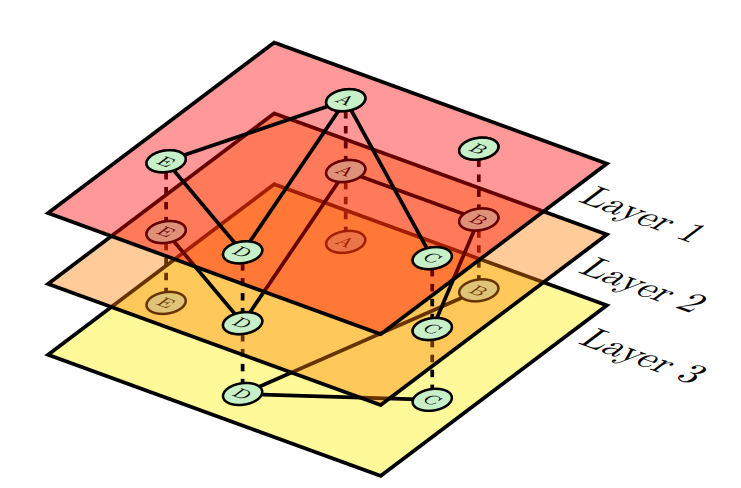
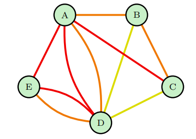
Multiplex networks are multilayer networks in which each layer is itself a network. In turn, the layers are connected by edges that connect nodes in different layers. A multiplex network includes two additional conditions: 1) the set of nodes on each layer is the same; and 2) interlayer edges only connect the same node between layers (Boccaletti et al. 2014). Multiplex networks are unique among multilayer networks in being capable of being represented as a multigraph, where there is a single set of nodes with potentially several edges joining any two nodes. Figure 1 is a multiplex network with a single set of nodes, A – E, that exist on each layer. Interlayer edges, the dotted connections, only exist between identical nodes in different layers. Figure 2 indicates how Figure 1 could be represented as a multigraph.
Applications to social network analysis
Multiplex networks are particularly useful in social network analysis because each node can be treated as an individual and each intralayer edge as a connection between two individuals. Treating each layer as a type of communication channel between individuals allows the network to represent many different types of interactions that would be overly simplified in a single-layer network (Assenova & Sridhar 2019; Battiston et al. 2016; Boccaletti et al. 2014; Cozzo et al. 2013; Gomez et al. 2013; Ruiz-Martin et al. 2020). Verbrugge (1979) has noted that adult friendships have different types of interactions that can only be modeled accurately by multiplex networks. Attempting to analyze a multiplex network as individual simplex (single-layer) networks produces results that lack the nuances of a multiplex network (De Domenico et al. 2015; Menichetti et al. 2014).
Network properties
The layers of a multiplex network are interdependent during warning dissemination, so an important aspect of initializing the network is deciding the number of layers (i.e., the number of communication channels). Modeling every type of communication channel as a unique layer may be intractable, requiring substantial computational complexity while providing a minimal impact on network entropy, especially for similar types of communication channels (De Domenico et al. 2015). However, combining multiple types of communication channel into a single layer may obscure subtle communities in the network (Mondragón et al. 2018). Some research analyzes the correlation of network edges between layers (Battiston et al. 2014; Bianconi 2013; Boccaletti et al. 2014). This correlation can identify similar layers, potentially allowing them to be joined into a single layer with minimal distortion of network structure (De Domenico et al. 2015).
Percolation theory
One important contribution to network analysis is percolation theory, which indicates that for a percentage \(p\) of nodes removed from a network, there exists a critical threshold \(p = p_c\) above which a large connected component exists and below which it does not exist (Chen et al. 2007). Previous research has analyzed social network percolation in the context of firms’ advertising (Campbell 2013), but this theory can also be applied to emergency warnings. Specifically, models of emergency warning networks can examine the effects of a warned individual’s probability \(p\) of sharing the warning with their peers. This produces site percolation, and a critical threshold of dissemination probability can be found above which the majority of the network will eventually be warned and below which only a minority will. However, little is known about the relationship between the number of initially warned nodes in a network and the critical threshold \(p_c\) where the majority of the network’s nodes eventually become warned.
Percolation in multiplex networks has been studied extensively (Cellai et al. 2013). One important aspect is the minimal set of initially warned nodes needed for percolation criticality (Morone & Makse 2015), which is relevant to warning dissemination. However, in this study we randomize the set of initially warned nodes, since the broadcast process may not be able to target a certain set of individuals specifically, either due to constraints in the communication channel or due to officials not knowing what the minimal set of individuals is in their community. Another aspect that affects percolation in a multiplex network is the structure of each layer. Yu et al. (2020) compared ER, SF, and SW random networks as different layers of a duplex (two-layer) diffusion network. This concept has also been generalized to multilayer networks, comparing structures of random graphs as they affect information diffusion (Wang et al. 2013). In addition to percolation regarding information diffusion, percolation of node failures has been assessed in multiplex networks (Danziger et al. 2016; Vaknin et al. 2020). While there may be some overlap of results with information diffusion, the largely stochastic nature of diffusion and differences in assumptions likely produces quite different results. Similarly, Chang & Fu (2019) analyzed the synergistic effects of multiple contagions in a multilayer network, but did not consider interlayer contagion, preventing an exact mapping to information diffusion.
Site and bond percolation
There are two primary approaches to percolation: site percolation and bond percolation. As described previously, site percolation involves removing \(p\) nodes from a network. Conversely, bond percolation involves removing \(p\) edges from a network. While this difference may appear minor, each type can produce different results (Radicchi & Castellano 2015). Nonetheless, warning dissemination can be modeled as site percolation since a node that fails to disseminate warnings is a "dead end" that produces the same warning propagation results as if it no longer existed in the warning network.
Discrete-event simulations
ABSs are commonly contrasted with discrete-event simulations (DESs), but the two types of simulations are not mutually exclusive (Chan et al. 2010; Maidstone 2012; Siebers et al. 2010). DESs are simulations which model time as a sequence of discrete events. DESs can be contrasted with continuous simulations, which model time on the basis of a set of continuous equations. Moreover, DES time progression can be separated into two types: fixed-increment and next-event. Fixed-increment time progression models each time step in the course of the simulation, allowing for consistent updates as time progresses. Next-event time progression models time in a series of events, moving forward to the next event after completing the current one. This allows for reduced computation in situations where updates would not occur at every time step with fixed-increment time progression. Accordingly, DES studies should use next-event time progression due to a potentially long latency between a node receiving a warning and later relaying it to others.
SEIR epidemiological model
The SIR epidemiological model is a compartmental model that has been used to analyze the spread of infectious diseases. Each component—S: susceptible, I: infectious, R: recovered—defines the state of an individual. A variant of the SIR model, the SEIR model, includes E: exposed. The order of the letters indicates the sequence of transitions between them. According to SEIR, an individual is initially susceptible to an infection. If they encounter an infected individual, they enter the exposed (E) stage, after which they can then transition to the infected (I) stage. Finally, the individual transitions to the recovered (R) stage, at which point they cannot infect others or become reinfected.
Similarities to emergency warning dissemination
Although the SEIR model was originally applied to epidemiology, it has also been applied to information dissemination (Bettencourt et al. 2006; Zhang et al. 2021) and is also similar to stages of warning dissemination described by disaster researchers (Lindell & Perry 2012). Table 1 shows how warning dissemination states can be defined as stages that are roughly equivalent to those in the SEIR model.
| SEIR | Warning stages |
|---|---|
| Susceptible | Access: Able to receive a warning through one or more communication channels |
| Exposed | Reception: Received a warning but is deciding whether to believe it |
| Infectious | Milling: Relaying the warning to others |
| Recovered | Response: Ceased warning others and either taking protective action or resuming normal activity |
Protective action decision model
The Protective Action Decision Model (PADM) is a framework to investigate how individuals commonly respond to environmental hazards. It consists of an initial awareness stage where individuals are accessible to and receive threat information from environmental cues (seeing a funnel cloud in the case of a tornado), social cues (seeing neighbors evacuating), or social warnings (messages received from information sources through communication channels); a milling stage where they assess the threat’s potential impacts on them and their communities; and a response stage where they either take protective action or resume normal activities (Lindell 2018; Lindell & Perry 2012). Two particularly important stages for an ABS of warning dissemination are the cue (access and reception) and milling stages, where people learn of a hazard and decide whether to warn others. However, it is also important to include an evacuation variable to account for the possibility that this response will force the agent to cease warning others by word-of-mouth.
Related work
This study attempts to find the effect of the number of initially warned nodes in the network on the critical threshold where the majority of the network has been warned. To do so, our ABS uses a multiplex social network to model emergency warning dissemination. Our model extends that of Hui et al. (2008), who focused on an ER network, and Hui et al. (2010), who compared two types of nodes with a trust differential in emergency warning dissemination. In their second study, Hui et al. (2010) used ER, BA, and WS networks to analyze the differences in their representations of the warning dissemination process. Other studies have conducted emergency warning dissemination simulations using household grids; both Nagarajan et al. (2010) and Nagarajan et al. (2012) used a grid of 1000 households, with Nagarajan et al. (2012) studying a spatial network.
Methods
Dissemination framework
The structure of interactions between individuals in the network and their decisions can be described by the dissemination framework depicted in Figure 3. The simulation begins with a broadcast process in which a fixed number of nodes are randomly selected from the network to be warned. Following this, the contagion process activates each newly warned node until it ceases to relay warnings.
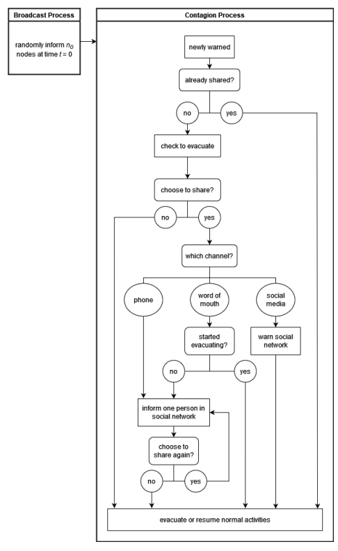
The simulation can be found at https://github.com/Wang-Research-Group/WarningDissem.jl or https://www.comses.net/codebase-release/89ba9886-1ebb-48cf-a288-53a0d7c0e2de/.
Simulation parameters
The parameters to the simulation have been informed by values provided by previous literature. This section describes the parameters and their informed values.
Broadcast size (\(n_0\))
The broadcast size is the initial number of nodes informed at the beginning of the simulation, prior to the contagion process. Previous research has provided broadcast sizes for a wide range of hazards including flash floods, water contamination, hurricanes, and volcanoes. However, since the relationship of this variable is to be compared with the probability of an individual to relay a warning, we test a wide range of values. Table 2 provides a brief summary of \(n_0\)’s properties.
| Parameter | \(n_0\) |
|---|---|
| Description | Broadcast size |
| Type | value |
| Range | [1, \(n\)] (\(n\) being number of nodes) |
For the Mount St. Helens (MSH) eruption Lindell & Perry (1987) identified 6% and 0% who received information from official sources in two locations and 58% and 47% who received information from their social network in those locations. These MSH numbers do not add to 100%, which indicates that many individuals were informed by other means such as environmental cues (e.g., seeing the ash cloud). While this may indicate a possible concern with assuming only social warnings in this simulation, many hazard types will not have as obvious environmental cues, and the sudden nature of the broadcast process indicates it could include those other types of information sources as well. Table 3 summarizes these literature values and others.
| Values | Hazard Type | Information Source | Source |
|---|---|---|---|
| 14% min, 38% median, 89% max | flash floods | peers | Lindell et al. (2019) |
| 31.8% | floods | primarily neighbors | Werritty et al. (2007) |
| 7%, 0% | hurricanes | peers | Lindell et al. (2021) |
| 6%, 0% | volcano | officials | Lindell & Perry (1987) |
| 58%, 47% | volcano | social network | Lindell & Perry (1987) |
Probability to relay the warning (\(p\))
The probability an informed individual will relay a warning to others is a very significant parameter of the simulation since it plays a major role in percolation. This simulation parameter is a function which takes four parameters: \(t_s\) (current time), \(d\) (total forewarning), \(t_l\) (time to relay the warning), and \(c\) (warning belief). The difference, \(d - t_s\), determines how much time is left before the disaster strikes. This value affects an individual’s probability to relay the warning because an individual receiving a warning a very short time before the disaster will cause them to tend to their own household’s safety before warning others. \(t_l\) plays a role in the probability to relay the warning because a series of warning options which take a long time will affect how much time an individual has to prepare themselves prior to the disaster. Finally, \(c\), warning confirmation, is important because an individual who has not confirmed a warning will be less likely to relay it. Table 4 provides a brief summary of \(p\)’s properties.
| Parameter | \(p\) |
|---|---|
| Description | Probability to relay a warning |
| Type | function |
| Function Parameters | \(t_s\), \(d\), \(t_l\), \(c\) |
| Output | value/distribution |
| Output Range | [0, 1] |
Based on these assumed parameters, we construct a function \(p\) to use for results; however, the simulation allows for an easy change of function for this simulation parameter. Equation 1 describes this function:
| \[ p(t_s, d, t_l, c) = c \times p_0 \times \text{max}\left(1 - \frac{\text{min}(t_l)}{\text{max}(d - t_s, 0)}, 0\right)\] | \[(1)\] |
This function has the property where a confidence of 0 or a time to communicate longer than the time remaining returns a result of 0. A returned value of \(p_0\) occurs when confidence is 100% and time to communicate is 0. We include the \(p_0\) for percolation purposes; since probability appears to vary widely among different communities, percolation changes drastically with small adjustments of \(p\), and the relationship with \(n_0\) is based on \(p\), we select a wide range of values and narrow them to determine the relationship.
While few studies provide information regarding what percentage of people informed someone else, several of them identify how many warned others via different communication channels. These studies can help guide starting values for this parameter before narrowing it down. One study which did have general information of how many people informed others identified 1.1% and 2.4% told someone else during two hazardous materials transportation accidents (hazmat accidents) (Rogers & Sorensen 1989). Other studies which are more specific regarding communication channels are detailed in Section 3.10 and Tables 6 and 7.
Probability to relay warning on communication channels (\(p_l\))
The weight to relay the warning on different layers (communication channels) determines how often each layer is used in warning dissemination. A higher value in one element of the vector increases the use of the given layer while decreasing the use of the others; in other words, the vector is the set of weights in the multiple layers. The parameter \(p_l\) is a function which takes three parameters: \(t_s\), \(d\), and \(t_l\). The difference \(d - t_s\) determines how much time remains before the disaster strikes. This value affects a layer’s weight for the same reason as it affects \(p\): receiving a warning shortly before the disaster strikes will cause people to tend to their own household’s safety before warning others outside the household. This combined with \(t_l\) identifies the effect that the time it takes to relay a warning via a given communication channel has on deciding to use it. Table 5 provides a brief summary of \(p_l\)’s properties.
| Parameter | \(p_l\) |
|---|---|
| Description | Probability to relay warning on communication channels |
| Type | function |
| Function Parameters | \(t_s\), \(d\), \(t_l\) |
| Output | list of values/distributions – one per layer |
| Output Range | [0, 1]; sum of values/sampled distributions \(= 1\) |
Based on these assumed parameters, we construct a function \(p_l\) to use for results; however, the simulation allows for an easy change of function for this simulation parameter. Equation 2 describes this function:
| \[ p_l(t_s, d, t_l) = \text{norm}\left(b \times \text{max}\left(1 - \frac{t_l}{\text{max}(d - t_s, 0)}, 0\right)\right)\] | \[(2)\] |
We include \(b\) to emphasize variation. Some communities may be predisposed towards certain communication channels where the time remaining before the disaster strikes and the time to transmit a message play negligible roles. In these cases, \(b\) allows for returning values which may appear closer to the community’s characteristics.
Communication probabilities with different types of communication channels are much more common in emergency warning literature than other communication domains. We separate these probabilities into two groups: probabilities of warned individuals relaying the warning to others via different types of communication channels (Table 6) and probabilities of individuals receiving the warning via different types of communication channels (Table 7). The latter group does not exactly correspond to the intent of \(p_l\); however, they can provide guidance on the values of the former group. “Hazmat” represents “hazardous materials transportation accidents”.
| Values | Hazard Type | Communication Channel | Source |
|---|---|---|---|
| 22% | floods | neighbors | Parker et al. (2009) |
| 27% | emergencies in Europe; survey | social media | Reuter & Spielhofer (2017) |
| 48% | emergencies in Europe; survey | social media in future | Reuter & Spielhofer (2017) |
| 0.1% | wildfire | retweets (Twitter) | Sutton et al. (2014) |
| 0.1% | tsunami | retweets (Twitter) | Chatfield et al. (2013) |
| 57.7% | tsunami | face-to-face | Perry (2007) |
| 26.9% | tsunami | phone call | Perry (2007) |
| 5.8% | tsunami | SMS | Perry (2007) |
| Values | Hazard Type | Communication Channel | Source |
|---|---|---|---|
| 1.84 (1-5 Likert scale) | hurricane | internet | Lindell et al. (2005) |
| 36% | flash flood | face-to-face | Mileti & Beck (1975) |
| 31.8% | floods | neighbors | Werritty et al. (2007) |
| 1.1% | floods | SMS | Werritty et al. (2007) |
| 10.5% | floods | not neighbors or SMS | Werritty et al. (2007) |
| 26% | tornado | word of mouth | Robinson et al. (2019) |
| 51% | tornado | cell phone | Robinson et al. (2019) |
| 8% | tornado | social media | Robinson et al. (2019) |
| 17% | tornado | internet | Robinson et al. (2019) |
| 18.3% | Hazmat | friends, neighbors, relatives | Rogers & Sorensen (1989) |
| 11.8%, 29.7% | Hazmat | door-to-door | Rogers & Sorensen (1989) |
| 24% | volcano | face-to-face | Lindell & Perry (1987) |
| 13%, 14% | volcano | telephone | Lindell & Perry (1987) |
Warning time (\(t_l\))
The time an individual takes to relay the warning can vary based on the communication channel they choose. In the real world there is also time it takes for an individual to receive information; depending on the communication channel, an individual who is away from their home or communication device can take longer to be warned. To simplify, in this study we include that additional time into \(t_l\). It is expected to have a minimal effect combined as opposed to separated, since individuals only attempt to communicate once. However, it could play a role in simulation parameters which use this variable in their functions if the effect of this variable is significant. The simplification of the parameter of warning time also allows for fewer limitations on literature values to be used. This is especially noticeable with social media, since many people may not receive a notification of the update. Table 8 summarizes \(t_l\)’s properties.
| Parameter | \(t_l\) |
|---|---|
| Description | Warning time |
| Type | list of values/distributions – one per layer |
| Range | [0, \(\infty\)) |
Table 9 summarizes previous literature values. Zhang et al. (2014b) did not explicitly provide the values included in the table except for the oral communication channel, although it seems they were a part of their data; we compute the values based on equations and tables. The delay time for microblog communication was computed with Equation 7 and Table 1 of the paper. Delay time for oral communication was said to be 1 minute, although this appears to be an assumption. The delay time for SMS and cell was indicated to be 99.2% closer to oral communication than microblog; based on this statement and the computed values of oral and microblog communication, SMS and cell communication was computed to be 17 minutes.
| Values | Hazard Type | Communication Type | Source |
|---|---|---|---|
| 3.36 hrs | disasters in Beijing; survey | microblog | Zhang et al. (2014b) |
| 1 min | disasters in Beijing; survey | oral | Zhang et al. (2014b) |
| 17 mins | disasters in Beijing; survey | SMS, cell | Zhang et al. (2014b) |
| 49 mins | Hazmat | friends, neighbors, relatives | Rogers & Sorensen (1989) |
| 70 mins, 66 mins | Hazmat | door-to-door | Rogers & Sorensen (1989) |
Warning verification (\(c\))
Warning confidence plays a significant role in informed individuals deciding to relay it to others. Many individuals will choose to verify information before trusting it, which produces a slower and less effective percolation process. An individual’s warning confidence depends on how many times they have received it previously, from which source, and their trust in that source. Based on these aspects, the simulation parameter \(c\) is a function which takes \(c_s\) and \(w_l\) as parameters. Table 10 provides a summary of its properties.
| Parameter | \(c\) |
|---|---|
| Description | Warning verification |
| Type | function |
| Function Parameters | \(c_s\), \(w_l\) |
| Output | value/distribution |
| Output Range | [0, 1] |
Based on these assumed parameters, we construct a function \(c\); however, the simulation allows for an easy change of function for this simulation parameter. Equation 3 describes this function:
| \[ c(c_s, w_l) = \text{clamp}\left(\frac{\text{trust}(c_s, w_l)}{c_n + 1}, 0, 1\right)\] | \[(3)\] |
We include \(c_n\) as the number of times an individual wishes to confirm a warning with others. Trust levels have a linear relationship with this value.
Previous research regarding confidence and confirmation is minimal. One paper specified an average number of confirmations, which is the most helpful for determining a range of values for \(c\), but others reported the communication channels from which confirmation was sought without providing any data regarding how much confirmation individuals required. Warning confidence data is challenging to acquire, since it requires public surveys to collect. Table 11 details some of the previous literature regarding warning confirmation.
| Values | Hazard Type | Communication Type | Source |
|---|---|---|---|
| confirmed with on avg 1.37 (std dev 0.65) | flash floods | N/A | Lindell et al. (2019) |
| confirmed with on avg 1.76 different warning channels | water contamination | N/A | Lindell et al. (2017) |
| 11.0%, 11.2% waited to see | Hazmat | N/A | Rogers & Sorensen (1989) |
| 31.3% confirmed | tsunami | face-to-face | Perry (2007) |
| 4.1% confirmed | tsunami | telephone | Perry (2007) |
| 3.1% confirmed | tsunami | internet | Perry (2007) |
Evacuation probability (\(r\))
Since protective actions by the public involve evacuating for many types of hazards, including an evacuation probability accounts for this likely scenario. Lindell et al. (2005) found that peers and local authorities were more important determinants of hurricane evacuation than were other information sources. In a wildfire context, individuals rated the influence of others telling them to evacuate as 3.50 on a 1–5 Likert scale (McCaffrey et al. 2018). A decision to evacuate involves the time remaining until the disaster strikes (\(d - t_s\)) and warning confidence (\(c\)), so the simulation parameter \(r\) is a function. Table 12 summarizes the properties of \(r\).
| Parameter | \(r\) |
|---|---|
| Description | Evacuation probability |
| Type | function |
| Function Parameters | \(t_s\), \(d\), \(c\) |
| Output | value |
| Output Range | [0, 1] |
Based on these assumed parameters, we construct a function \(r\); however, the simulation allows for an easy change of function for this simulation parameter. Equation 4 describes this function:
| \[ r(t_s, d, c) = c \times \left(1 - \text{clamp}\left(\frac{d - t_s}{t_r}, 0, 1\right)\right)\] | \[(4)\] |
This function has the property where the probability to evacuate is 0 if the time remaining until the disaster strikes is greater than \(t_r\) and the probability is 1 if the time remaining until the disaster strikes is 0 or has already passed. We include \(t_r\) as the maximum time (i.e., the earliest) at which anyone would evacuate.
Previous literature does not detail the probability of an individual evacuating at any given time; rather, it provides results of times that they leave. The literature is best suited for validating evacuation results, although it can guide potential testing values. The majority of evacuation literature considers hurricanes. Some evacuation departure time studies have reported that hurricane evacuations follow a Rayleigh distribution, with studies using \(\beta\) parameters of 40, 45, 62, 74, 117, and 181 (Lindell and Prater 2007).
Forewarning (\(d\))
The amount of forewarning before a disaster strikes plays a major role in warning dissemination. An extremely short forewarning causes individuals to look after their own household’s safety rather than informing others as well as limits the length of the chain of receiving a warning and relaying the warning to others. A longer forewarning allows for flexibility on both of these fronts. Since forewarning before a disaster is fixed at the start of the contagion process, the simulation parameter \(d\) is constant throughout a given simulation. Table 13 summarizes \(d\)’s properties.
| Parameter | \(d\) |
|---|---|
| Description | Forewarning before disaster |
| Type | value |
| Range | (0, \(\infty\)) |
While the warning dissemination time literature is primarily based on tsunami and hurricane hazards, their corresponding forewarning times are expected to be on the shortest and longest ranges of hazard values, respectively. Table 14 summarizes several study values.
| Values | Hazard Type | Source |
|---|---|---|
| 9 mins | tsunami | Chatfield et al. (2013) |
| 12 mins | tsunami | Anderson (1969) |
| 72 hrs | hurricane | Lindell et al. (2021) |
| 42 hrs | hurricane | Lindell et al. (2005) |
| 36 hrs | hurricane | US Department of Commerce, NOAA (2019) |
Warning confidence (\(w_l\))
To determine warning confidence, an individual will evaluate their trust in the source. While a source will be another individual, the type of social connection the two people have may be correlated with their communication channel. Several studies have grouped trust into communication types (Tandoc et al. 2020; Zhang et al. 2014b; Zhang et al. 2016), allowing for a simplified manner of adjusting trust levels. This simulation does the same, with a simulation parameter \(w_l\). Table 15 summarizes its properties.
| Parameter | \(w_l\) |
|---|---|
| Description | Trust of layers |
| Type | list of values/distributions – one per layer |
| Range | [0, 1] |
Table 16 details literature on trust in social networks. All studies except for source Rogers & Sorensen (1989) group trust by communication channel. Zhang et al. (2016) do not indicate where their values originate; presumably a survey was conducted.
| Values | Value location | Communication Channel | Source |
|---|---|---|---|
| 81.3%, 58.6% disregarded information | hazardous materials transportation accidents | N/A | Rogers & Sorensen (1989) |
| 2.74 trustworthy (1–5 Likert scale) | news in Singapore | social media | Tandoc et al. (2020) |
| 45% | disasters in Beijing | Zhang et al. (2016) | |
| 50% | disasters in Beijing | microblog | Zhang et al. (2016) |
| 41.3% | disasters in Beijing; survey | SMS | Zhang et al. (2014b) |
| 43.3% | disasters in Beijing; survey | cell phone | Zhang et al. (2014b) |
| 38.91% | disasters in Beijing; survey | oral | Zhang et al. (2014b) |
| 48.3% | disasters in Beijing; survey | microblog | Zhang et al. (2014b) |
Network structure
An advantage of a multiplex network is the ability to customize each layer with unique properties. The literature summarized in Tables 2–16 suggests that there are generally three types of communication channels: 1) one-to-one physical interaction, such as face-to-face (word-of-mouth) communication with neighbors; 2) one-to-one virtual interaction, such as voice phone calls; and 3) one-to-many virtual interaction, such as social media (e.g., Twitter and Facebook). We have labeled these three generalized communication channels word-of-mouth, phone, and social media, respectively, but recognize that these are simplified labels for more complex categories. For example, smart phones can be used for SMS and email, both of which can be used to relay warnings to multiple individuals simultaneously. Similarly, social media can also include retweets, microblog, and internet posts. Although these three categories do not capture the nuances of all available communication channels, they provide a reasonable representation of the major types of communication channels. Each layer has specific characteristics that are detailed in the following sections.
An undirected network
Each layer of the multiplex social network is modeled as an undirected network, which is the type that has been assumed in previous warning dissemination studies (Hasan & Ukkusuri 2011; Sadri 2016) and assumes a reciprocal relationship for all layers. Although a form of social media might be designed such that “following” others might not be reciprocal within informal warning networks, we assume that these cases are somewhat rare.
One important aspect of an undirected network is that a newly warned node could attempt to recontact their warning source. Indeed, warning recipients sometimes do recontact their original warning sources to seek or provide additional information about the threat and protective actions (Wood et al. 2018). However, to simplify the analyses that follow, we provisionally assume that this possibility does not significantly affect the warning dissemination process.
Phone layer
This simulation limits the phone layer to one-to-one voice communication (i.e., ignoring the one-to-multiple capabilities of text and email), which yields a network with the Watts-Strogatz (WS) model’s small-world property. Phone-type networks have indeed been shown to have the small-world property (Amblard et al. 2015; Miklas et al. 2007; Wang et al. 2016) and very high coverage, with one study citing 97.2% for SMS and 99.0% for cell phone (Zhang et al. 2014b). The same study also provided the average number of people forwarded to for different communication types: 11.8 on SMS and 9.7 on voice phone calls. Wang et al. (2016) identified a phone network as a WS network with an average node degree of 6 and rewiring probability of 0.7. By contrast, Miklas et al. (2007) identified a network with an average node degree of 20. To account for these widely varying values, we set the phone layer to have a rewiring probability of 0.7 and an average node degree of 10, which is the middle of the range between 6 and 20, and is approximately the same as the average number of people warned.
The number of people warned by phone depends on previous warning success. If an individual decides to warn, they do so and check their probability again, repeating until they cease attempting. The expected number of people warned is \(\frac{p}{1 - p}\) since the behavior is the inverse of a geometric distribution. Note that, like the undirected network case, there is a possibility that an individual will attempt to contact the same person twice. This feature is consistent with people monitoring a threatening situation (e.g., an approaching hurricane) by repeatedly exchanging information with trusted others in the milling process (Lindell et al. 2019; Wood et al. 2018).
Word-of-mouth layer
Previous studies have incorporated spatial features into social networks (Amblard et al. 2015), so we set the simulation’s word-of-mouth layer as a random geometric graph (RGG) based on real-world data. Coverage is essentially perfect, with one study citing 100% for oral communication (Zhang et al. 2014b). Our real-world data is drawn from two sources: a possible population distribution of Seaside, Oregon (Wang et al. 2016) and household locations approximated by 2020 census data for Coos Bay, Oregon (United States Census Bureau 2020). Both of these locations are coastal communities that are vulnerable to a Cascadia Subduction Zone tsunami. Using real-world data yields a spatial network with a realistic clustering structure. The cutoff value used for the RGG is 60 meters because Zhang et al. (2014b) found the distribution of oral communication was entirely within 90 meters, with the vast majority, 93.6%, within 60 meters. Based on this finding, we allow for connections between any individuals within 60 meters.
Although real-world warning responses are typically made by households comprising multiple individuals, we represent each household as a single individual. This is clearly a reasonable approximation when all household members are together at home—as is typically the case during evenings and weekends. In such cases, warning dissemination within households takes place face-to-face at (essentially) zero distance and, thus, is virtually instantaneous. However, representing each household as a single individual is also a reasonable approximation if household members are separated during weekdays because people try to contact each other to verify that all members are aware of the hazard (e.g., Jon et al. 2016). That is, the probability of warning propagation within separated households is approximately \(p = 1.0\), which is much higher than the probability of warning propagation between households. Although warning propagation within households may delay warning propagation between households, the delay will not have a significant effect on the overall warning process if separated household members have independent access to broadcast warnings (and thus, experience no delay in warning receipt) or are in social contexts such as workplaces where warnings propagate face-to-face as rapidly as in households. Thus, at least as a first approximation, modeling households as single individuals is likely to decrease ABS processing time without reducing the accuracy of the results.
For a stable diffusion process, studies have used 600 nodes in Hui et al. (2008), 1000 in Nagarajan et al. (2010), Nagarajan et al. (2012), and Watts et al. (2019), and 10000 and 20000 in DiCarlo & Berglund (2021). Based on these values, the node sizes of 26363 for Coos Bay and 4502 for Seaside appear suitable for this simulation study.
The word-of-mouth layer is affected by the evacuation parameter \(r\). When an individual evacuates, they are removed from this layer because, having evacuated, they can no longer talk directly to neighbors. However, they can still communicate virtually via phone or social media, so those layers are unaffected by evacuation.
The number of people contacted to relay a warning depends on previous contact success. If an individual decides to relay a warning, they do so and check their probability again, repeating until they cease contacting others. This is the same behavior as for the phone layer. Similarly, the expected number of people contacted is \(\frac{p}{1 - p}\) since the behavior is the inverse of a geometric distribution and there is a possibility the individual will attempt to recontact the same person as part of the milling process.
Social media layer
We set the social media layer of the simulation as a scale-free network using the Barabási–Albert (BA) model, consistent with the findings of previous research (Amblard et al. 2015; Aparicio et al. 2015; Zhang et al. 2021). Coverage is much lower than in phone and word-of-mouth networks: 66.5% in Zhang et al. (2014b), 63% in Reuter & Spielhofer (2017), 47.7% in Sadri et al. (2017), 24.7% in Sadri et al. (2017), and 12.5% in Perry (2007). Because of this wide range of values, our analyses also included a case of no social media. The average number of people contacted to relay a warning is much higher than in phone networks (Zhang et al. 2014a) because social media is a limited form of broadcast channel. That is, when an individual decides to warn people via social media, they broadcast it to everyone in their social media network. This allows for matching forwarding number and average node degree and provides an advantage of social media over the other two personal communication channels.
The parameters of the BA model are the number of initial nodes in the network before adding edges and the number of edges added for each new node. We choose values of \(0.374n\) and 105 respectively, with \(n\) being the total number of nodes (26363 for Coos Bay or 4502 for Seaside). To select these values we chose a range of possible parameter values and compared resulting coverage and average node degree. These values give approximately 63% coverage and an average node degree of 132, which match the coverage and forwarding numbers in the literature.
The Julia programming language
This simulation is written in the Julia programming language. Julia is a high-level dynamically typed language designed for high performance numerical computing (Bezanson et al. 2017). Used heavily in academic research, it provides high-level language features similar to Python with lower-level features such as parallelism. A recent Julia package for ABSs, Agents.jl (Datseris et al. 2022), has aided in developing ABSs in Julia such as those in Douven & Hegselmann (2021) and Basurto et al. (2020).
The simulation uses several packages which make the core simulation much simpler:
- Graphs (Fairbanks et al. 2021): mathematical graphs and utility functions
- MetaGraphs: functionality on top of Graphs to support node properties
- Distributions (Besançon et al. 2021): probability distributions and utility functions
- DataFrames: tabular data storage similar to R’s dataframes
- DataStructures: tree and queue data structures
- CSV: importing and exporting data to/from CSV files
- JLSO (Finnegan & White 2020): importing and exporting data to/from JLSO files (compressed data type)
- Makie: plotting
- Colors: colorschemes for plotting
- ProgressMeter: progress tracking on the terminal
Results and Examples
Simplified example
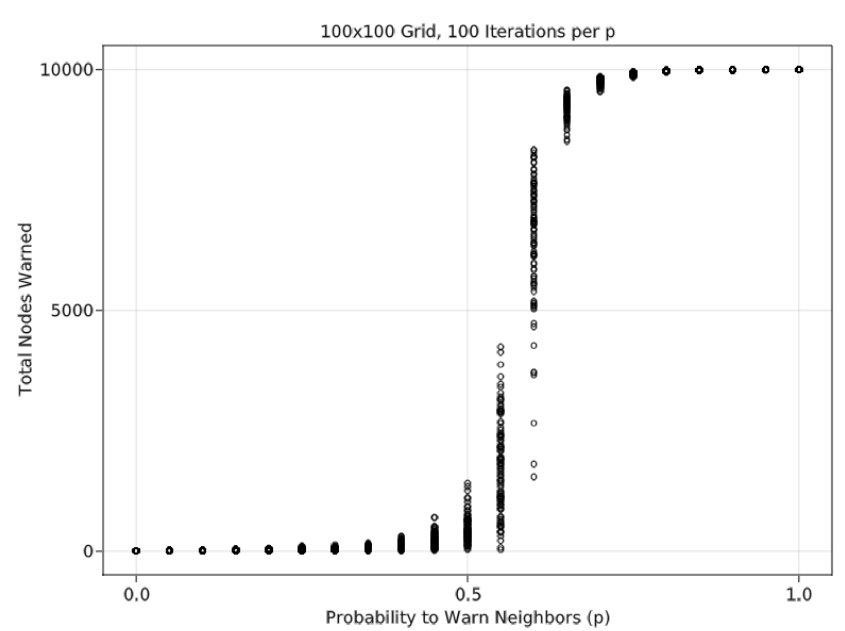
To illustrate our search for a relationship between \(n_0\) (broadcast size) and a critical value of \(p\) (probability to relay the warning), we provide a simplified example of our ABS using a lattice grid and ER network. In this simplified example, the only two variables are \(n_0\) and \(p\), there is a single layer of the network, and warning relay only occurs with two connected nodes. Based on these properties, a lattice grid network has a theoretical critical percolation threshold of 50%. Figure 4 shows results of the simulation where \(n_0 = 10\) (out of 10000 nodes). Moreover, a Monte Carlo analysis performed over different values of \(p\) (probability to relay a warning to a peer), with 100 iterations per \(p\) value, indicates that the simulated critical threshold matches the theoretical value. Figure 5 shows the same results over different levels of \(n_0\); as \(n_0\) increases, the critical percolation threshold decreases. \(n_0\) and \(p\) values for this example were chosen to display a wide range of possible scenarios.
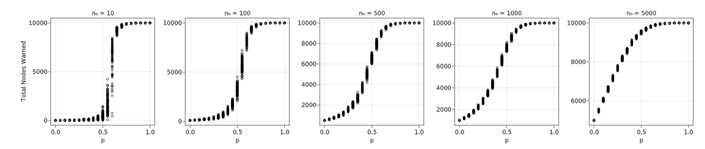
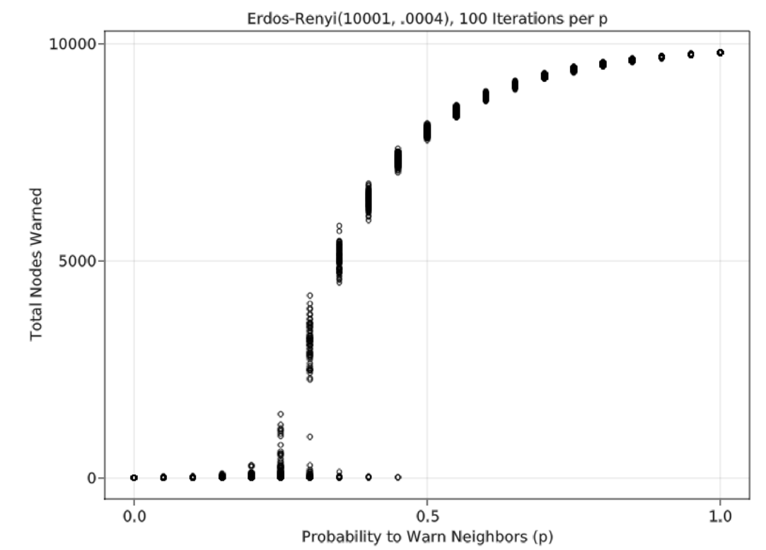
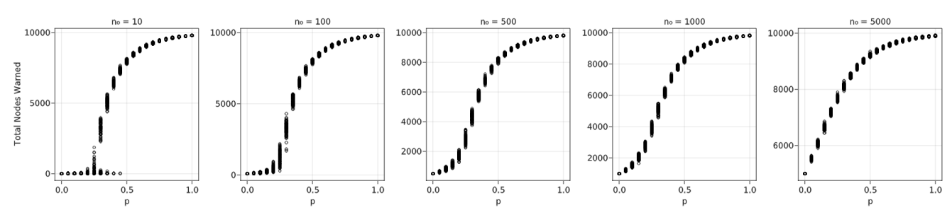
The tests for the lattice grid were replicated in an ER network having a node size of 10000, the same as the lattice grid, and an average node degree of 4. Based on these properties, this ER network has a theoretical critical percolation threshold of 25%. Figure 6 shows that a simulation in which \(n_0 = 10\) yields a critical threshold that matches the theoretical value. Unlike the lattice grid network, low \(n_0\) values yield some results that are close to 0 even with relatively high \(p\) values. These results are due to the nature of the random network; with only 10 initially warned nodes, there is a chance that several have a low degree, increasing the chances that all 10 of them will fail to spread the warning. The lattice grid network could have the same results, but it is relatively rare with only 100 Monte Carlo iterations. Figure 7 shows the same results as Figure 6 over different levels of \(n_0\). Like the lattice grid network, as \(n_0\) increases, the critical percolation threshold decreases.
Full simulation
We start with an exploratory sensitivity analysis of all simulation parameters, followed by a narrower and more detailed view of a few key parameters. For simplicity, in this section the values for the simulation parameters \(p\), \(p_l\), \(c\), and \(r\) are initial starting parameters we designed for the provided functions: \(p_0\), \(b\), \(c_n\), and \(t_r\). Additional information on these initial starting parameters can be found in equations 1, 2, 3, and 4. Table 17 details the range of values used for the first exploratory analysis of the Coos Bay dataset (\(n\) = 26363). Each combination of parameter values has four Monte Carlo iterations. The ordering of the values in the lists of simulation parameters \(p_l\), \(t_l\), and \(w_l\) are [phone, word-of-mouth, social media], corresponding to the ABS’s three layers. The chosen values originate from the literature values detailed in Section 3.3; to have consistent coverage of the simulation parameter space, we selected values within the range of those reported in the literature and center the values at those most commonly cited. The third value of \(p_l\), [30%, 70%, 0%], is not derived from the literature. Instead, we selected those values to account for a scenario where social media is unavailable or internet coverage is sparse. Only a single value of \(c\) is available from the literature, so we selected values two standard deviations away from a mean of 1.37, which was obtained from Lindell et al. 2019. If \(c\) is a random variable following a normal distribution, that encompasses approximately 95% of the population.
| Simulation Parameter | Description | Range of Values |
|---|---|---|
| \(n_0\) (Section 3.4) | broadcast | 1582, 7909, 13182, 18454, 24518 (6%, 30%, 50%, 70%, 93%) |
| \(p\) (Section 3.6) | probability | 5%, 20%, 35%, 50%, 65%, 80% |
| \(p_l\) (Section 3.10) | channel probability | [50.5%, 25.5%, 24%], [2.5%, 73.3%, 24.2%], [30%, 70%, 0%] |
| \(t_l\) (Section 3.14) | sharing time | [17 mins, 1 min, 120 mins], [120 mins, 70 mins, 201.6 mins] |
| \(c\) (Section 3.16) | confidence | 0.07, 2.67 |
| \(r\) (Section 3.20) | evacuation | 15 mins, 60 mins, 360 mins, 3600 mins (60 hrs), 5760 mins (96 hrs) |
| \(d\) (Section 3.24) | forewarning time | 9 mins, 60 mins, 180 mins, 1440 mins (24 hrs), 4320 mins (72 hrs) |
| \(w_l\) (Section 3.26) | trust | [43%, 39%, 48%] |
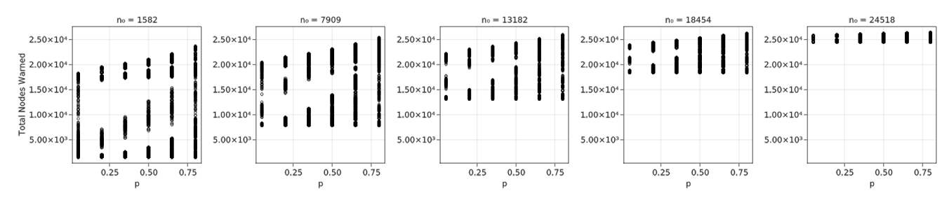
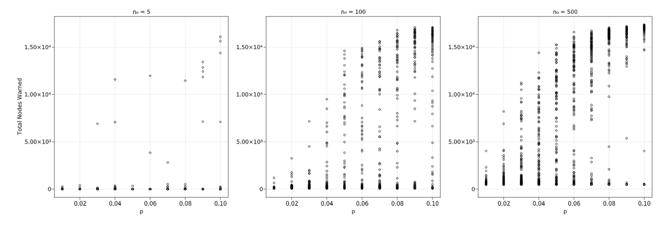
When examining a range of \(n_0\) values between 1582 (6%) and 24518 (93%) out of 26363, Figure 8 indicates that the variation across the \(p\) values is mostly a linear trend. This, combined with a very large variation of total nodes informed at the smallest value of \(p\) (5%), indicates a closer look is needed at smaller values of \(n_0\) and \(p\).
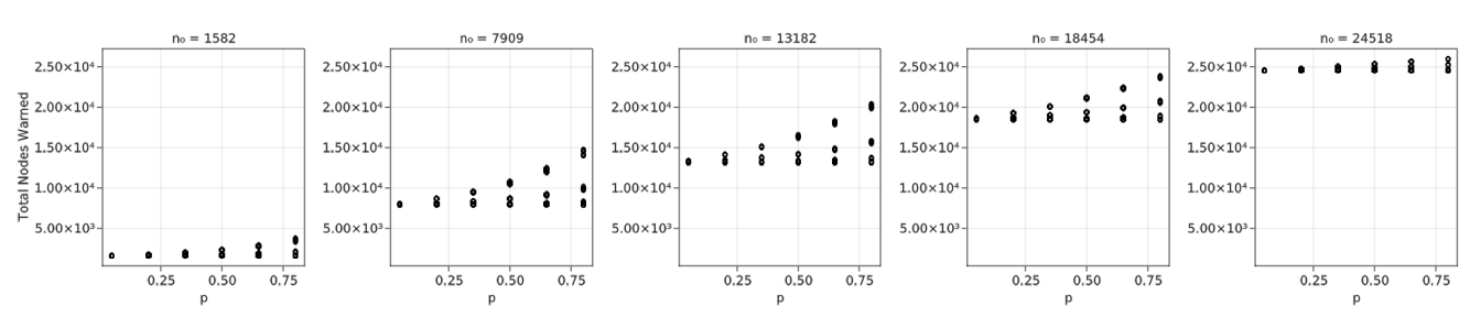
Specifically, Figure 9, with 100 Monte Carlo iterations per combination, \(n_0 =\) 5, 100, 500, and \(p =\) 1–10%, begins to show the expected curve. Particularly, \(n_0 =\) 500 looks somewhat similar to Figure 6, although with much more variation. This analysis has most variables fixed to single values for computational time purposes, unlike Figure 8.
Using the exploratory data, we analyzed the sensitivity of simulation parameters other than \(n_0\) and \(p\), beginning with \(d\)—the amount of forewarning time before disaster impact. Figure 10 indicates that the contagion process when \(d = 9\) min performs poorly, even with high \(n_0\). The largest difference between the initial and final numbers of warned nodes is 7268, approximately 28% of the total. Unsurprisingly, this result indicates that extremely rapid onset hazards such as local tsunamis should not rely on a contagion process and will likely perform better with immediate broadcast methods such as tone alert radio or SMS notification. Moreover, environmental cues for a local tsunami such as recognizing long/strong earthquake shaking and social cues such as seeing neighbors evacuating can supplement local tsunami warning broadcasts (Chen et al. 2021). Further analyses use a \(d\) value of 1440 min (24 hr) since it is shorter than hurricane forewarning times but long enough to show the contagion process for some hazards such as nuclear power plant accidents. We also use \(n_0 = 1582 \, (6\%)\) and \(p = 5\)% because of Figure 9’s indication of the critical percolation threshold at low \(n_0\) and \(p\) values.
The value of \(c\) significantly impacts total nodes warned. Table 18 shows an approximately tripling of final dissemination values for the lower \(c = 0.07\), indicating that a lower requirement for warning confirmation increases total nodes warned. Although there is a notable difference in the values, we continue to use \(c = 0.07\) since lack of trust in a source may additionally lower warning confidence. Literature summarized in Table 11 displays the average number of confirmations during dissemination, which implicitly includes trust levels and situational uncertainty.
| \(c\) Value | Min | Mean | Median | Max |
|---|---|---|---|---|
| 0.07 | 1608 | 10461 | 13814 | 17596 |
| 2.67 | 1613 | 4158 | 3617 | 14318 |
Although not impacting total nodes warned nearly as much as variation in \(c\), variation in \(t_l\) still makes a notable difference. This is likely because every value in the second list for \(t_l\), [120 min, 70 min, 201.6 min], is longer than the corresponding value in the first list. This means the minimum value in the first list is considerably smaller than the corresponding one in the second list, affecting \(p\) as shown in Equation 1. Table 19 summarizes the differences in values. Note that the order of layers in the list is [phone, word-of-mouth, social media]. For further analysis, we used \(t_l =\) [17 min, 1 min, 202 min] because those values are more directly based on the empirical literature and, with the word-of-mouth value being considerably smaller, are likely more sensitive to evacuations.
| \(t_l\) Value | Min | Mean | Median | Max |
|---|---|---|---|---|
| [17 mins, 1 min, 120 mins] | 1616 | 11460 | 16993 | 17596 |
| [120 mins, 70 mins, 201.6 mins] | 1608 | 9463 | 12328 | 16399 |
As indicated in Table 20, changes in \(r\) do not appear to impact total nodes warned. This is surprising considering the impact that evacuation has on word-of-mouth dissemination. It implies the most important communication channels are phone and social media. For additional analysis, we use \(r = 3600\) min (60 hr) because it is not the largest value but it is greater than \(d\). A value greater than \(d\) means that some individuals will choose to evacuate immediately (Lindell and Prater 2007).
| \(r\) Value | Min | Mean | Median | Max |
|---|---|---|---|---|
| 15 mins | 1647 | 11810 | 16778 | 17579 |
| 60 mins | 1642 | 11836 | 17057 | 17596 |
| 360 mins | 1648 | 10916 | 17071 | 17539 |
| 3600 mins (60 hrs) | 1622 | 12008 | 17054 | 17587 |
| 5760 mins (96 hrs) | 1616 | 10727 | 16897 | 17432 |
Table 21 reveals a significant difference in total nodes warned between when social media is approximately 24% and when it is 0. The two results when social media is approximately 24% are quite similar, although it appears that the condition with a larger phone percentage produces slightly more nodes warned. This table indicates that social media plays a large role in warning dissemination and phone communication plays a somewhat larger role than word-of-mouth. These results suggest that communities with limited internet access may need to supplement the informal warning process with additional official communication channels such as NOAA Weather Radio or provide resources to increase effectiveness of the informal warning process. For further analysis, we use \(p_l =\) [50.5%, 25.5%, 24%]. The values in the list originate from previous literature and the differences between values are smaller than the other two lists.
| \(p_l\) Value | Min | Mean | Median | Max |
|---|---|---|---|---|
| [50.5%, 25.5%, 24%] | 17161 | 17343 | 17312 | 17587 |
| [2.5%, 73.3%, 24.2%] | 16982 | 17053 | 17054 | 17123 |
| [30%, 70%, 0%] | 1622 | 1629 | 1630 | 1634 |
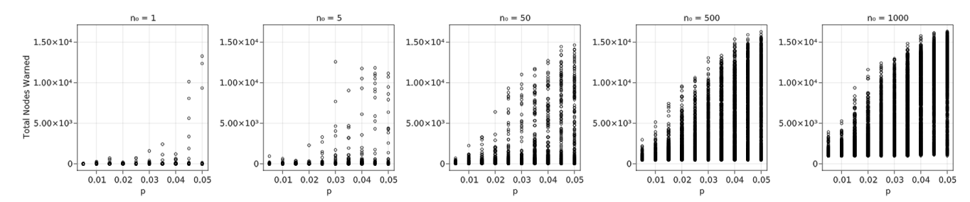
Since reference values for all variables have been identified, we analyze \(n_0\) and \(p\) in additional detail. Figure 11 shows 50 different combinations of \(n_0\) and \(p\), with \(n_0 =\) 1, 5, 50, 500, and 100 and \(p =\) 1–5%. Due to the low probabilities and highly stochastic nature of the problem, results vary significantly across each run of the simulation. Consequently, we conducted a much larger number of iterations to identify a curve when there are low values of \(n_0\) and \(p\). The results for 1000 Monte Carlo iterations show that, with \(n_0 = 1\), the vast majority of results are very close to 0; only a few approach larger numbers similar to those seen with larger \(n_0\). Based on this figure, it appears that a critical percolation threshold may be around 3.5–4%. As \(n_0\) increases, the critical threshold appears to shift to the left, toward smaller \(p\). For example, when \(n_0 = 50\) the threshold appears to be around 1.5% and at \(n_0 = 1000\) it is closer to 0.5–1%. While these differences appear significant in determining a necessary initial broadcast size, the critical threshold cannot necessarily be relied upon; with such small \(p\), the variation is large and there are still many simulation runs in which the critical percolation threshold is close to 0 even with larger \(n_0\). The result for \(n_0 = 1000\) in Figure 11 indicates there is a steady range of results within each \(p\) value even with the smaller critical percolation threshold.
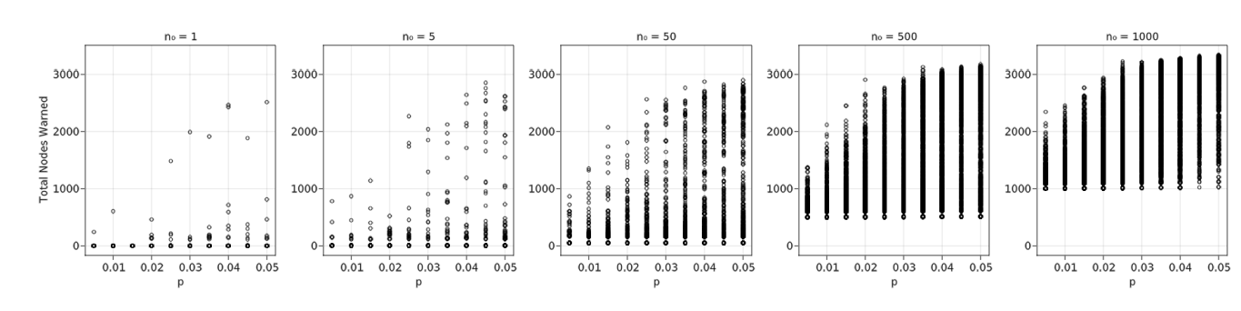
The data in Figure 11 was replicated with Seaside data to produce Figure 12. While the exact critical thresholds may not be quite as obvious, they seem to follow the same trend as the Coos Bay data. Note that while the \(n_0\) values are the same between the two datasets, they are different percentages of each community’s total population since Coos Bay has 26363 individuals and Seaside has 4502.
Validation
Some simulation parameters, being functions, do not have direct connections to existing literature, so this section analyzes values produced during the simulation to assess their similarity to previous studies’ results. We begin by examining differences in real probability values from the initial starting \(p\). Since the initial starting \(p\) is used for analysis in the Results section, any results drawn from those conclusions need to be adjusted for these differences. The differences are provided in Table 22 for \(p =\) 0.5–5% in the Coos Bay dataset. Note that the real probability values are always less than \(p\) due to the function detailed in Equation 1. As \(p\) increases, the differences in probabilities also increase, greater than a constant fraction of \(p\). The differences are small, with the greatest being three-quarters of 1%. This indicates that, while the \(p\) values shown in Figures 11 and 12 are not exact, they are close enough that the trends identified previously remain.
| Initial Starting \(p\) | Mean Difference in Real Value from \(p\) (always less) |
|---|---|
| 0.005 | 0.0001 |
| 0.010 | 0.0005 |
| 0.015 | 0.0010 |
| 0.020 | 0.0017 |
| 0.025 | 0.0027 |
| 0.030 | 0.0034 |
| 0.035 | 0.0046 |
| 0.040 | 0.0056 |
| 0.045 | 0.0065 |
| 0.050 | 0.0075 |
While relatively small \(p\) values have been identified for the critical percolation threshold, we use larger ones when analyzing hurricane dissemination times. Lindell et al. (2021) identified peers as the first source of warning in 7% and 0% of the population in two different hurricanes. Because of this, we use the exploratory \(p =\) 5%, 20%, 35%, 50%, 65%, 80%. In a hurricane scenario with \(d =\) 1440 min (24 hr), 4320 min (72 hr), the average percentage of the population informed after 8 hr is 87%, quite a bit higher than the 70% identified in the literature (Lindell et al. 2021). The average percentage informed after 24 hours is 89%, fitting the \(>\) 80% found in the same study. An additional study found that 50% were warned by 15 min and 95% were warned by 2.25 hr (Lindell et al. 2005). The simulation finds an average 51% warned by 15 min and 79% by 2.25 hr. The combination of over- and under-estimation by the simulation when compared with previous studies shows that the results are within acceptable bounds.
Lindell et al. (2005) found that approximately 53.6% of the risk area residents evacuated from Hurricane Lili. The simulation calculates an average of 35% evacuated in hurricane forewarning times of \(d =\) 1440 min (24 hr), 4320 min (72 hr). This appears quite a bit smaller than the empirical value from the research literature; however, the simulation produces a range of 30–94%, showing a difference of 18.6% may not be as large as it originally appears.
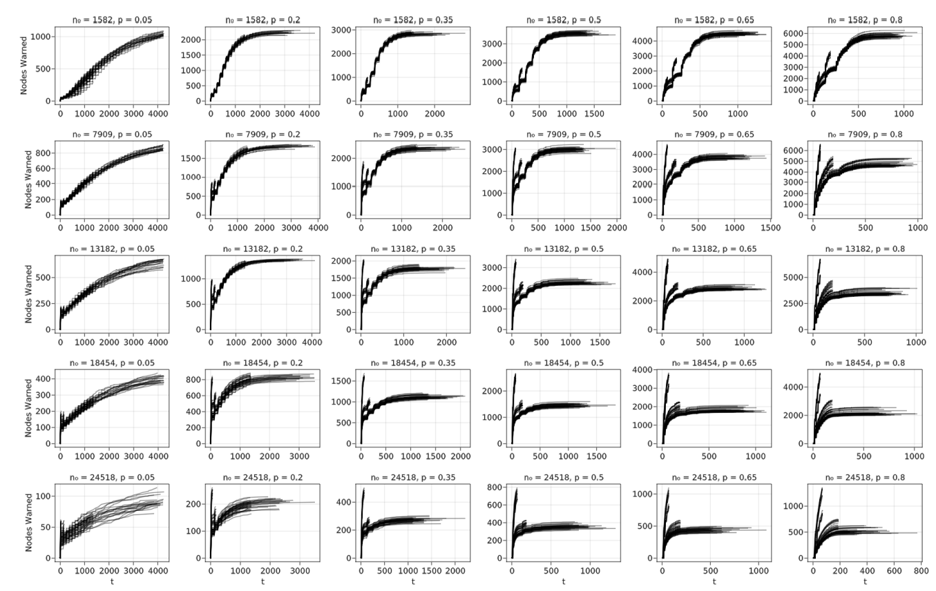
Zhang et al. (2014a) provided a dissemination curve of individuals warned by phone, but they did not provide many specific parameters of their model, so we selected a range of \(n_0 =\) 1582, 7909, 13182, 18454, 24518 (6%, 30%, 50%, 70%, 93%), \(p =\) 5%, 20%, 35%, 50%, 65%, 80%, \(d =\) 9 min, 60 min, 180 min, 1440 min (24 hr), 4320 min (72 hr), and \(r =\) 15 min, 60 min, 360 min, 3600 min (60 hr), 5760 min (96 hr). These are all from the exploratory values of Table 17. Figure 13 shows the results, which do not seem to match the Zhang et al. (2014a) sigmoidal telephone dissemination curve. This is likely due to differences in warning dissemination behavior. In the present study’s simulation, an individual continues to contact others until failure, which has an expected value of \(\frac{p}{1 - p}\) contacts, since it is inverse of a geometric distribution. By contrast, Zhang et al. (2014a) have an individual attempt to contact 150 others, regardless of failure. In addition, our simulation has word-of-mouth and social media layers in addition to a phone layer, so the additional two layers also contribute to the differences in the two studies’ results.
Discussion
While the methods and results of this study make a significant contribution to the literature on warning modeling, there are assumptions made, often due to complexity constraints, that could be addressed by future research. We address limitations and future research below.
Limitations and future research
Our ABS makes seven primary simplifying assumptions, some of which deviate from the findings of behavioral research on warnings. These are 1) limiting the ABS to eight simulation parameters (\(n_0\), \(p\), \(p_l\), \(t_l\), \(c\), \(r\), \(d\), and \(w_l\)) and determining the relationships between them (as described in Section 3.2); 2) assuming reciprocal relationships with an undirected network; 3) ignoring the amount of time that it takes authorities to decide to issue warnings Sorensen (2020); 4) combining time to communicate and time before receiving a warning—especially problematic with word-of-mouth because it is not easy to “leave a message” if the recipient is not there; 5) assuming that disaster requires evacuation and that evacuation is explicitly recommended in the warning (recommendations to shelter in-place during a hazmat incident might produce different warning dissemination dynamics); 6) assuming that evacuation terminates the word-of-mouth communication channel; and 7) assuming a household behaves like a single individual.
Broadcast process
The broadcast process has six additional major assumptions that could be addressed in future research, the first of which is that there is exactly one broadcast source, but many hazards elicit warnings from multiple sources that can transmit a mixture of accurate information, inadvertent misinformation, and deliberate disinformation. This raises the issue of varying levels of trust in different sources. The second assumption is that the broadcast is transmitted through a single channel, but it has long been known that authorities use multiple warning channels of their own (e.g., sirens and NOAA Weather Radio), as well as multiple TV and radio stations (Drabek 1986). The third assumption is that the broadcast is transmitted only at the beginning of the incident, rather than repeatedly through the period of forewarning. This is especially unrealistic for slower-onset hazards. In such situations, researchers such as Mileti & Peek (2000) have advised community officials to broadcast messages repeatedly to increase the percentage of those at risk who have received a warning. The fourth assumption is that every individual in the broadcast process receives a warning instantly (and, thus, at the same time), but broadcast warning reception can be spread out over an extended period of time (Lindell et al. 2021). The fifth assumption is that any broadcast message that is received is also heeded and understood but this is not necessarily the case—especially when risk area residents do not understand the language in which the broadcast is transmitted (Lindell 2018). The sixth assumption is that every individual in the broadcast process has complete trust in official sources, regardless of the communication channel or message content. However, as noted earlier, even those who receive an official broadcast warning tend to try to confirm it (Drabek 1986).
Warning sources
This study also neglects a number of aspects of warning sources other than the official broadcast process and the informal contagion process. The first simplifying assumption is that there are no environmental or social cues—or, alternatively, that risk area residents fail to recognize their significance. This is sometimes the case for tsunamis in which people are unaware that long and strong earthquake shaking is a reliable cue to an imminent tsunami. The second simplifying assumption is that the milling process comprises only warning relay, when in fact it also includes the confirmation of existing information and search for additional information (Wood et al. 2018), as well as evacuation preparation activities (Lindell et al. 2019). The third simplifying assumption is that trust is attributed to communication channels rather than warning sources. This might be realistic when people receive a text message directly from a public safety agency, but is not necessarily the case for other channels.
Social context
In addition, these simulations ignored the time of day at which an emergency warning is delivered. This is an important consideration because it can affect the length of time before individuals receive a warning (Krings et al. 2012). Specifically, time of day affects people’s access to different communication channels and day of week affects whether household members are separated when danger threatens (Lindell et al. 2017).
Network structure and parameters
As yet, the structure of the social networks for different types of communities remains unclear, so future work could test the possible effects of directed networks with different types of structures such as regular or ER networks. If choosing to use different data sources for the word-of-mouth layer, locations that are inland and more rural may provide additional insights. Finally, validating the current simulation parameter functions is extremely important for evaluating the sensitivity of the variables. For example, the seemingly discrete curves of Figure 13 indicate there may not be enough variation in the simulation parameters for smooth curves. Future work could determine the variation in parameters necessary for curves more suitable for regression analysis.
Conclusions
We developed an ABS that modeled warning dissemination in a multiplex social network where each layer is a different communication channel. We used data from the empirical warning literature to define suitable parameter values for the simulation and verify its results. Providing real-world data as a context for a hazard, we used a dataset for Seaside, OR (H. Wang et al. 2016) and 2020 census data to inform a dataset of Coos Bay, OR (United States Census Bureau 2020).
The simulation results show that an initial official broadcast of an emergency warning plays a significant role in the subsequent spread of the warning through the contagion process. Although several characteristics of the situation affect the warning dissemination process—such as amount of forewarning before a disaster strikes, the likelihood of warning confirmation, and the amount of time it takes to relay warnings—the most significant is the probability that an individual will relay a warning to others.
We began to validate the ABS results by showing that they are consistent with empirical findings from warning research. When applying all considered variables in the model to a more complex simulation, the results indicate that, as expected, initial broadcast size has a negative correlation with the critical percolation threshold. The threshold ranges from approximately 1–5%, where a larger initial broadcast lowers the value. Other significant variables include probability to share the warning, confidence in the warning, and amount of time remaining until the disaster strikes. Social media appears to play a large role in warning dissemination as well, suggesting a possibly highly effective method for rapid warning dissemination, provided it is checked often and is considered to be trustworthy.
This study’s most immediate contribution is to advance the state of the art in warning modeling beyond the recent analysis of empirical warning dissemination curves presented in Lindell et al. (2021) and experimental framework on peer influence provided by Linardi (2016). Although the Lindell et al. (2021) analysis summarized the available research on hurricane warnings, it was only able to provide warning dissemination curves that were aggregated across communities and events. The present study extends that analysis by providing a capability to tailor analyses of warning time distributions to the distinctive characteristics of each hazard and the unique set of warning channels in each community. Nonetheless, future research needs to refine the model described here to better represent people’s known patterns of behavior when disasters threaten their communities.
This study’s longer term contribution is to advance the state of the art in models of emergency warning dissemination. Specifically, further studies of this type can provide guidance to local officials in their efforts to warn local residents as disasters threaten, given the unique characteristics of their community and the hazards they face. Continuing research on the official broadcast and informal contagion processes will provide more specific results and policy suggestions. Simulation models of emergency warning dissemination will become increasingly relevant as communities face increasingly challenging environmental hazards (Cramton 2021; Jones et al. 2020; Laska & Morrow 2006).
Acknowledgements
The authors would like to acknowledge the funding support from the National Science Foundation through grants: #1826407, #1902888, #1826455, #1952792, #2044098, #2052930, and #2103713. Any opinions, findings, and conclusion or recommendations expressed in this research are those of the authors and do not necessarily reflect the view of the funding agencies. We would also like to show our gratitude to anonymous reviewers for the constructive suggestions and comments.References
ALAM, S. J., & Geller, A. (2012). Networks in agent-based social simulation. In A. J. Heppenstall, A. T. Crooks, L. M. See, & M. Batty (Eds.), Agent-Based Models of Geographical Systems (pp. 199–216). Berlin Hiedelberg: Springer.
ALBERT, R., & Barabási, A. L. (2002). Statistical mechanics of complex networks. Reviews of Modern èhysics, 74(1), 47.
AMBLARD, F., Bouadjio-Boulic, A., Gutiérrez, C. S., & Gaudou, B. (2015). Which models are used in social simulation to generate social networks? A review of 17 years of publications in JASSS. IEEE 2015 Winter Simulation Conference (WSC). Available at: https://hal.science/hal-01303799/document.
ANDERSON, W. A. (1969). Disaster warning and communication processes in two communities. Journal of Communication, 19(2), 92–104.
APARICIO, S., Villazón-Terrazas, J., & Álvarez, G. (2015). A model for scale-free networks: Application to Twitter. Entropy, 17(8), 5848–5867.
ASSENOVA, V. A., & Sridhar, N. (2019). Multiplex network diffusion. Working Paper, The University of Pennsylvania.
BARABÁSI, A. L., & Bonabeau, E. (2003). Scale-free networks. Scientific American, 288(5), 60–69.
BASURTO, A., Dawid, H., Harting, P., Hepp, J., & Kohlweyer, D. (2020). Economic and epidemic implications of virus containment policies: Insights from agent-based simulations. Bielefeld Working Papers in Economics and Management
BATTISTON, F., Iacovacci, J., Nicosia, V., Bianconi, G., & Latora, V. (2016). Emergence of multiplex communities in collaboration networks. PloS ONE, 11(1), e0147451.
BATTISTON, F., Nicosia, V., & Latora, V. (2014). Structural measures for multiplex networks. Physical Review E, 89(3), 032804.
BESANÇON, M., Papamarkou, T., Anthoff, D., Arslan, A., Byrne, S., Lin, D., & Pearson, J. (2021). Distributions.jl: Definition and modeling of probability distributions in the JuliaStats ecosystem. Journal of Statistical Software, 98(16), 1–30.
BETTENCOURT, L. M., Cintrón-Arias, A., Kaiser, D. I., & Castillo-Chávez, C. (2006). The power of a good idea: Quantitative modeling of the spread of ideas from epidemiological models. Physica A: Statistical Mechanics and Its Applications, 364, 513–536.
BEZANSON, J., Edelman, A., Karpinski, S., & Shah, V. B. (2017). Julia: A fresh approach to numerical computing. SIAM Review, 59(1), 65–98.
BIANCONI, G. (2013). Statistical mechanics of multiplex networks: Entropy and overlap. Physical Review E, 87(6), 062806.
BIRKBAK, A. (2012). Crystallizations in the blizzard: Contrasting informal emergency collaboration in Facebook groups. Proceedings of the 7th Nordic Conference on Human-Computer Interaction: Making Sense Through Design.
BOCCALETTI, S., Bianconi, G., Criado, R., Del Genio, C. I., Gómez-Gardenes, J., Romance, M., Sendina-Nadal, I., Wang, Z., & Zanin, M. (2014). The structure and dynamics of multilayer networks. Physics Reports, 544(1), 1–122.
CAMPBELL, A. (2013). Word-of-mouth communication and percolation in social networks. American Economic Review, 103(6), 2466–2498.
CELLAI, D., López, E., Zhou, J., Gleeson, J. P., & Bianconi, G. (2013). Percolation in multiplex networks with overlap. Physical Review E, 88(5), 052811.
CHAN, W. K. V., Son, Y.-J., & Macal, C. M. (2010). Agent-based simulation tutorial-simulation of emergent behavior and differences between agent-based simulation and discrete-event simulation.
CHANG, H.-C. H., & Fu, F. (2019). Co-contagion diffusion on multilayer networks. Applied Network Science, 4(1), 1–15.
CHATFIELD, A. T., Scholl, H. J. J., & Brajawidagda, U. (2013). Tsunami early warnings via Twitter in government: Net-savvy citizens’ co-production of time-critical public information services. Government Information Quarterly, 30(4), 377–386.
CHEN, C., Lindell, M. K., & Wang, H. (2021). Tsunami preparedness and resilience in the Cascadia Subduction Zone: A multistage model of expected evacuation decisions and mode choice. International Journal of Disaster Risk Reduction, 59, 102244.
CHEN, Y., Paul, G., Cohen, R., Havlin, S., Borgatti, S. P., Liljeros, F., & Stanley, H. E. (2007). Percolation theory and fragmentation measures in social networks. Physica A: Statistical Mechanics and Its Applications, 378(1), 11–19.
CHEN, Z. (2019). An agent-based model for information diffusion over online social networks. Papers in Applied Geography, 5(1–2), 77–97.
CONOVER, M. D., Davis, C., Ferrara, E., McKelvey, K., Menczer, F., & Flammini, A. (2013). The geospatial characteristics of a social movement communication network. PloS ONE, 8(3), e55957.
COZZO, E., Banos, R. A., Meloni, S., & Moreno, Y. (2013). Contact-based social contagion in multiplex networks. Physical Review E, 88(5), 050801.
CRAMTON, P. (2021). Lessons from the 2021 Texas electricity crisis. Utility Dive, 23.
DANZIGER, M. M., Shekhtman, L. M., Berezin, Y., & Havlin, S. (2016). The effect of spatiality on multiplex networks. EPL (Europhysics Letters), 115(3), 36002.
DATSERIS, G., Vahdati, A. R., & DuBois, T. C. (2022). Agents. jl: A performant and feature-full agent-based modeling software of minimal code complexity. Simulation.
DE Domenico, M., Lancichinetti, A., Arenas, A., & Rosvall, M. (2015). Identifying modular flows on multilayer networks reveals highly overlapping organization in interconnected systems. Physical Review X, 5(1), 011027.
DE Domenico, M., Nicosia, V., Arenas, A., & Latora, V. (2015). Structural reducibility of multilayer networks. Nature Communications, 6(1), 1–9.
DICARLO, M. F., & Berglund, E. Z. (2021). Connected communities improve hazard response: An agent-based model of social media behaviors during hurricanes. Sustainable Cities and Society, 69, 102836.
DOUVEN, I., & Hegselmann, R. (2021). Mis-and disinformation in a bounded confidence model. Artificial Intelligence, 291, 103415.
DRABEK, T. E. (1986). Human System Responses to Disaster. Berlin Heidelberg: Springer.
DUGDALE, J., Saoud, N. B. B., Zouai, F., & Pavard, B. (2016). Coupling agent based simulation with dynamic networks analysis to study the emergence of mutual knowledge as a percolation phenomenon. Journal of Systems Science and Complexity, 29(5), 1358–1381.
FAIRBANKS, J., Besançon, M., Schölly, S., Hoffiman, J., Eubank, N., & Karpinski, S. (2021). JuliaGraphs/Graphs.jl: An optimized graphs package for the Julia programming language. Available at: https://github.com/JuliaGraphs/Graphs.jl/.
FINNEGAN, R., & White, L. (2020). invenia/JLSO.jl. Available at: https://doi.org/10.5281/zenodo.3992374.
GOMEZ, S., Diaz-Guilera, A., Gomez-Gardenes, J., Perez-Vicente, C. J., Moreno, Y., & Arenas, A. (2013). Diffusion dynamics on multiplex networks. Physical Review Letters, 110(2), 028701.
GONZALEZ de Durana, J. M., Barambones, O., Kremers, E., & Varga, L. (2014). Agent based modeling of energy networks. Energy Conversion and Management, 82, 308–319.
HASAN, S., & Ukkusuri, S. V. (2011). A threshold model of social contagion process for evacuation decision making. Transportation Research Part B: Methodological, 45(10), 1590–1605.
HOU, J., Gai, W.-m., Cheng, W.-y., & Deng, Y.-f. (2020). Statistical analysis of evacuation warning diffusion in major chemical accidents based on real evacuation cases. Process Safety and Environmental Protection, 138, 90–98.
HUI, C., Goldberg, M., Magdon-Ismail, M., & Wallace, W. A. (2008). Micro-simulation of diffusion of warnings. Proceedings of the 5th International Conference on Information Systems for Crisis Response and Management ISCRAM2008.
HUI, C., Goldberg, M., Magdon-Ismail, M., & Wallace, W. A. (2010). Simulating the diffusion of information: An agent-based modeling approach. International Journal of Agent Technologies and Systems (IJATS), 2(3), 31–46.
JON, I., Lindell, M. K., Prater, C. S., Huang, S.-K., Wu, H.-C., Johnston, D. M., Becker, J. S., Shiroshita, H., Doyle, E. E., Potter, S. H., McClure, J., & Lambie, E. (2016). Behavioral response in the immediate aftermath of shaking: Earthquakes in Christchurch and Wellington, New Zealand, and Hitachi, Japan. International Journal of Environmental Research and Public Health, 13(11), 1137.
JONES, M. W., Smith, A., Betts, R., Canadell, J. G., Prentice, I. C., & Le Quéré, C. (2020). Climate change increases risk of wildfires. ScienceBrief Review, 116, 117.
KAPUCU, N., & Garayev, V. (2016). Structure and network performance: Horizontal and vertical networks in emergency management. Administration & Society, 48(8), 931–961.
KIESLING, E., Günther, M., Stummer, C., & Wakolbinger, L. M. (2012). Agent-based simulation of innovation diffusion: A review. Central European Journal of Operations Research, 20(2), 183–230.
KRINGS, G., Karsai, M., Bernhardsson, S., Blondel, V. D., & Saramäki, J. (2012). Effects of time window size and placement on the structure of an aggregated communication network. EPJ Data Science, 1(1), 1–16.
LINARDI, S. (2016). Peer coordination and communication following disaster warnings: An experimental framework. Safety Science, 90, 24–32.
LINDELL, M. K. & Perry, R. W. (1983). Nuclear power plant emergency warning: How would the public respond? Available at: https://www.researchgate.net/publication/236480964_Nuclear_power_plant_emergency_warning_How_would_the_public_respond.
LINDELL, M. K. (2018). Communicating imminent risk. In H. Rodríguez, E. L. Quarantelli, & R. R. Dynes (Eds.), Handbook of disaster research (pp. 449–477). Berlin Heidelberg: Springer.
LINDELL, M. K., Arlikatti, S., & Huang, S.-K. (2019). Immediate behavioral response to the June 17, 2013 flash floods in Uttarakhand, North India. International Journal of Disaster Risk Reduction, 34, 129–146.
LINDELL, M. K., Huang, S.-K., & Prater, C. S. (2017). Predicting residents’ responses to the may 1–4, 2010, boston water contamination incident. International Journal of Mass Emergencies and Disasters, 35, 84–113.
LINDELL, M. K., Lu, J.-C., & Prater, C. S. (2005). Household decision making and evacuation in response to Hurricane Lili. Natural Hazards Review, 6(4), 171–179.
LINDELL, M. K., Murray-Tuite, P., Wolshon, B., & Baker, E. J. (2019). Large-scale evacuation: The analysis, modeling, and management of emergency relocation from hazardous areas. London: Routledge.
LINDELL, M. K., & Perry, R. W. (1987). Warning mechanisms in emergency response systems. International Journal of Mass Emergencies and Disasters, 5(2), 137–153.
LINDELL, M. K., & Perry, R. W. (1992). Behavioral foundations of community emergency planning. Taylor & Francis.
LINDELL, M. K., & Perry, R. W. (2012). The protective action decision model: Theoretical modifications and additional evidence. Risk Analysis: An International Journal, 32(4), 616–632.
LINDELL, M. K., & Prater, C. S. (2007). Critical behavioral assumptions in evacuation time estimate analysis for private vehicles: Examples from hurricane research and planning. Journal of Urban Planning and Development, 133(1), 18–29.
LINDELL, M. K., Prater, C. S., & Peacock, W. G. (2007). Organizational communication and decision making for hurricane emergencies. Natural Hazards Review, 8(3), 50–60.
LINDELL, M. K., Sorensen, J. H., Baker, E. J., & Lehman, W. P. (2021). Community response to hurricane threat: Estimates of warning diffusion time distributions. Natural Hazards Review, 22(2), 04021007.
MACAL, C. M., & North, M. J. (2005). Tutorial on agent-based modeling and simulation. Proceedings of the Winter Simulation Conference, 2005.
MAIDSTONE, R. (2012). Discrete event simulation, system dynamics and agent based simulation: Discussion and comparison. System, 1(6), 1–6.
MCCAFFREY, S., Wilson, R., & Konar, A. (2018). Should i stay or should i go now? or should i wait and see? influences on wildfire evacuation decisions. Risk Analysis, 38(7), 1390–1404.
MENG, X., Zerfos, P., Samanta, V., Wong, S. H., & Lu, S. (2007). Analysis of the reliability of a nationwide short message service. IEEE INFOCOM 2007-26th IEEE International Conference on Computer Communications.
MENICHETTI, G., Remondini, D., Panzarasa, P., Mondragón, R. J., & Bianconi, G. (2014). Weighted multiplex networks. PloS ONE, 9(6), e97857.
MIKLAS, A. G., Gollu, K. K., Chan, K. K., Saroiu, S., Gummadi, K. P., & De Lara, E. (2007). Exploiting social interactions in mobile systems. International Conference on Ubiquitous Computing.
MILETI, D. S., & Beck, E. M. (1975). Communication in crisis: Explaining evacuation symbolically. Communication Research, 2(1), 24–49.
MONDRAGÓN, R. J., Iacovacci, J., & Bianconi, G. (2018). Multilink communities of multiplex networks. PloS ONE, 13(3), e0193821.
MORONE, F., & Makse, H. A. (2015). Influence maximization in complex networks through optimal percolation. Nature, 524(7563), 65–68.
NAGARAJAN, M., Shaw, D., & Albores, P. (2010). Informal dissemination scenarios and the effectiveness of evacuation warning dissemination of households — A simulation study. Procedia Engineering, 3, 139–152.
NAGARAJAN, M., Shaw, D., & Albores, P. (2012). Disseminating a warning message to evacuate: A simulation study of the behaviour of neighbours. European Journal of Operational Research, 220(3), 810–819.
PARKER, D. J., Priest, S. J., & Tapsell, S. M. (2009). Understanding and enhancing the public’s behavioural response to flood warning information. Meteorological Applications: A Journal of Forecasting, Practical Applications, Training Techniques and Modelling, 16(1), 103–114.
PERRY, S. D. (2007). Tsunami warning dissemination in Mauritius. Journal of Applied Communication Research, 35(4), 399–417.
RABERTO, M., Cincotti, S., Focardi, S. M., & Marchesi, M. (2001). Agent-based simulation of a financial market. Physica A: Statistical Mechanics and Its Applications, 299(1–2), 319–327.
RADICCHI, F., & Castellano, C. (2015). Breaking of the site-bond percolation universality in networks. Nature Communications, 6(1), 1–7.
RAHMANDAD, H., & Sterman, J. (2008). Heterogeneity and network structure in the dynamics of diffusion: Comparing agent-based and differential equation models. Management Science, 54(5), 998–1014.
RAND, W., Herrmann, J., Schein, B., & Vodopivec, N. (2015). An agent-based model of urgent diffusion in social media. Journal of Artificial Societies and Social Simulation, 18(2), 1.
REUTER, C., & Spielhofer, T. (2017). Towards social resilience: A quantitative and qualitative survey on citizens’ perception of social media in emergencies in Europe. Technological Forecasting and Social Change, 121, 168–180.
ROBINSON, S. E., Pudlo, J. M., & Wehde, W. (2019). The new ecology of tornado warning information: A natural experiment assessing threat intensity and citizen-to-Citizen information sharing. Public Administration Review, 79(6), 905–916.
ROGERS, G. O., & Sorensen, J. H. (1988). Diffusion of emergency warnings. Environmental Professional, 10(4), 185–198.
ROGERS, G. O., & Sorensen, J. H. (1989). Warning and response in two hazardous materials transportation accidents in the US. Journal of Hazardous Materials, 22(1), 57–74.
RUIZ-MARTIN, C., Wainer, G., & Lopez-Paredes, A. (2020). Discrete-Event modeling and simulation of diffusion processes in multiplex networks. ACM Transactions on Modeling and Computer Simulation (TOMACS), 31(1), 1–32.
SADRI, A. M., Ukkusuri, S. V., & Gladwin, H. (2017). The role of social networks and information sources on hurricane evacuation decision making. Natural Hazards Review, 18(3), 04017005.
SIEBERS, P.-O., Macal, C. M., Garnett, J., Buxton, D., & Pidd, M. (2010). Discrete-event simulation is dead, long live agent-based simulation! Journal of Simulation, 4(3), 204–210.
SORENSEN, J. H., Lindell, M. K., Baker, E. J. & Lehman, W. P. (2020). Community response to hurricane threat: Estimates of warning issuance time distributions.Weather, Climate and Society, 12 837–846.
SUTTON, J., Spiro, E. S., Johnson, B., Fitzhugh, S., Gibson, B., & Butts, C. T. (2014). Warning tweets: Serial transmission of messages during the warning phase of a disaster event. Information, Communication & Society, 17(6), 765–787.
TAYLOR, J. G., Gillette, S. C., Hodgson, R. W., Downing, J. L., Burns, M. R., Chavez, D. J., & Hogan, J. T. (2007). Informing the network: Improving communication with interface communities during wildland fire. Human Ecology Review, 14(2), 198–211.
UNITED States Census Bureau. (2020). QuickFacts: United States; Crescent City city, California; North Bend city, Oregon; Coos Bay city, Oregon. Available at: https://www.census.gov/quickfacts/fact/table/US,crescentcitycitycalifornia,northbendcityoregon,coosbaycityoregon/PST045219.
US Department of Commerce, NOAA. (2019). Hurricane and tropical storm watches, warnings, advisories and outlooks. National Weather Service. Available at: https://www.weather.gov/safety/hurricane-ww.
VAKNIN, D., Gross, B., Buldyrev, S. V., & Havlin, S. (2020). Spreading of localized attacks on spatial multiplex networks with a community structure. Physical Review Research, 2(4), 043005.
VERBRUGGE, L. M. (1979). Multiplexity in adult friendships. Social Forces, 57(4), 1286–1309.
WANG, H., Mostafizi, A., Cramer, L. A., Cox, D., & Park, H. (2016). An agent-based model of a multimodal near-field tsunami evacuation: Decision-making and life safety. Transportation Research Part C: Emerging Technologies, 64, 86–100.
WANG, J., Jiang, C., Quek, T. Q., WANG, X., & Ren, Y. (2016). The value strength aided information diffusion in socially-aware mobile networks. IEEE Access, 4, 3907–3919.
WANG, P., Robins, G., Pattison, P., & Lazega, E. (2013). Exponential random graph models for multilevel networks. Social Networks, 35(1), 96–115.
WATTS, D. J., & Strogatz, S. H. (1998). Collective dynamics of “small-world” networks. Nature, 393(6684), 440–442.
WATTS, J., Morss, R. E., Barton, C. M., & Demuth, J. L. (2019). Conceptualizing and implementing an agent-based model of information flow and decision making during hurricane threats. Environmental Modelling & Software, 122, 104524.
WERRITTY, A., Houston, D., Ball, T., Tavendale, A., & Black, A. (2007). Exploring the social impacts of flood risk and flooding in Scotland. Scottish Executive, Central Research Unit.
WOOD, M. M., Mileti, D. S., Bean, H., Liu, B. F., Sutton, J., & Madden, S. (2018). Milling and public warnings. Environment and Behavior, 50, 535–566.
XIONG, H., Payne, D., & Kinsella, S. (2018). Identifying mechanisms underlying peer effects on multiplex networks. Journal of Artificial Societies and Social Simulation, 21(4), 6.
YANG, Y., Mao, L., & Metcalf, S. S. (2019). Diffusion of hurricane evacuation behavior through a home-workplace social network: A spatially explicit agent-based simulation model. Computers, Environment and Urban Systems, 74, 13–22.
YU, Q., YU, Z., & Ma, D. (2020). A multiplex network perspective of innovation diffusion: An information-Behavior framework. IEEE Access, 8, 36427–36440.
ZHANG, M., Qin, S., & Zhu, X. (2021). Information diffusion under public crisis in BA scale-free network based on SEIR model — Taking COVID-19 as an example. Physica A: Statistical Mechanics and Its Applications, 571, 125848.
ZHANG, N., Huang, H., & Su, B. (2016). Comprehensive analysis of information dissemination in disasters. Physica A: Statistical Mechanics and Its Applications, 462, 846–857.
ZHANG, N., Huang, H., Su, B., & ZHANG, B. (2014). Analysis of different information dissemination ways for disaster prewarning: A case study of Beijing. Proceedings of the 3rd International Conference on Multimedia Technology (ICMT 2013)
ZHANG, N., Huang, H., Su, B., Zhao, J., & ZHANG, B. (2014). Information dissemination analysis of different media towards the application for disaster pre-warning. PloS ONE, 9(5), e98649.
ZHU, X., Song, J., Meng, J., & Liu, J. (2018). Information spreading in social network through explosive percolation theory. International Conference on Computational Social Networks