A Geospatial Bounded Confidence Model Including Mega-Influencers with an Application to Covid-19 Vaccine Hesitancy

Anna Haensch; Natasa Dragovic; Christoph Borgers; Bruce Boghosian

doi:10.18564/jasss.5027

Introduction

Opinions drive human behavior (Sîrbu et al. 2017), and opinion formation is a complex multi-scale process, involving characteristics of the individual, local interaction of individuals, social media, mass media, etc. Opinion dynamics have been modeled using approaches inspired by physics (van der Hofstad 2016). For surveys of the literature on opinion dynamics see for instance Lorenz (2007), Proskurnikov & Tempo (2018), and Mastroeni et al. (2019).

Opinions are formed in part by people talking to their families, friends, colleagues, etc. This is the sort of mechanism that the bounded confidence model of Hegselmann & Krause (2002) aims to capture. It is just one of several opinion dynamics models that have appeared in the literature; see for instance Ben-Naim (2005) Fortunato et al. (2005), Gargiulo & Gandica (2017), Urbig (2003) for others. However, our work here starts with the Hegselmann-Krause model.

Hegselmann & Krause (2015) augmented their model to include the impact of "radicals" on opinion formation. By their definition, a "radical" is an individual (or a group of individuals) holding an opinion that is extreme (at one end of the opinion spectrum) and unchanging. Matthias et al. (2016) proposed another model including radicals. Our Opinion Dynamics Network (ODyN) model includes "radicals" as well. We call them mega-influencers, thinking of mass media, prominent politicians, etc., and assuming that a mega-influencer is heard by a large fraction of the population.

To a model of opinion space dynamics with mega-influencers in the style of earlier work such as Hegselmann & Krause (2015) and Matthias et al. (2016), we add the new feature of geospatial dynamics. Closeness in two-dimensional space can be thought of as a stand-in for different notions of closeness; for instance, close family members might be considered "nearby" even when they live on a different continent. However, despite the seemingly geography-less nature of the online world, studies have shown (Lengyel et al. 2015) that geographic distance remains a key component in the formation and maintenance of social networks. For an extensive review on spatial networks, see Barthélemy (2011); the networks that we propose here are similar to the hidden variable model for spatial networks presented in Section 3 of Barthélemy (2011), but futher include bounded confidence.

We assume that individuals who are further apart from each other in two-dimensional space are less likely to influence each others’ opinions; this is reminiscent of the geometric inhomogeneous random graphs of Bringmann et al. (2015). The addition of a notion of spatial proximity turns out to have a very interesting effect: Large-scale geospatial patterns evolve out of random initial data. That is, spatial clusters of like-minded agents (think "blue states" and "red states") emerge, regardless of initialization.

Finally, we introduce the assumption that different people have different levels of influence, as in a Chung-Lu random graph (Chung & Lu 2002b, 2002a, 2004). Combing all of these factors, we can compute the probability that two agents speak during a given timestep and update their beliefs accordingly, similar to the random interactions of Weisbuch et al. (2002). As a result, opinion clusters no longer reach perfectly tight consensus with time, but rather, remain loosely spread around one or more dominant opinion centers.

We do not primarily intend to model digital social networks. Social media interactions can be akin to conversations among friends, family, neighbors, colleagues, in other words the sort of interactions modeled by the original Hegselmann-Krause model. However, social media users can also be mega-influencers; think of a Twitter account with millions of followers.

We construct a random graph reflecting all the features and assumptions discussed above. Vertices represent individuals, and directed edges indicate who influences whom. (When individual $v$’s opinion influences that of individual $u$, this does not necessarily imply that $u$ also influences $v$.)

In the simulations presented here, the spatial domain is a triangle, and the spatial locations of individuals are independent of each other and uniformly distributed. The code in the ODyN library also allows simulations on unions of triangles, where the number of individuals in each triangle is chosen to be random, Poisson-distributed, with an expected value proportional to the area of the triangle, possibly with different constants of proportionality for different triangles. In short, the spatial locations in the ODyN library are a Poisson point process with a possibly space-dependent rate.

As an example, we consider opinions about Covid-19 vaccination, a topic of urgent current interest for which data are plentiful. By April 19, 2021, vaccination was approved for everyone in the US age 16 and older. Despite the fact that the vaccine was free to all residents of the US, many factors impeded widespread vaccination. There was a lack of availability and access to vaccines in rural areas (Murthy et al. 2021), and vaccine hesitancy was impacted by fear of rare but severe vaccine side-effects (Beatty et al. 2021), social and economic factors (Simas & Larson 2021), as well as targeted misinformation campaigns and politicization of issues surrounding the vaccine (Rabb et al. 2022). Others have worked on bounded confidence models and spread of misinformation, for instance see (Douven & Hegselmann 2021). Such models are different from our model, in that they require the presence of a "ground truth," and therefore there is a concept of mis- and dis-information. In that and similar works the focus is on how best to organize communities of interacting agents in the presence of a fixed goal informed by the ground truth, and how to achieve this goal most efficiently (Douven 2019, 2022; Douven & Wenmackers 2017; Rosenstock et al. 2017; Zollman 2007). However, when the question is whether or not to accept a Covid vaccine, there is no objective, unquestionable "ground truth."

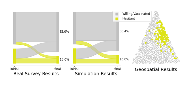
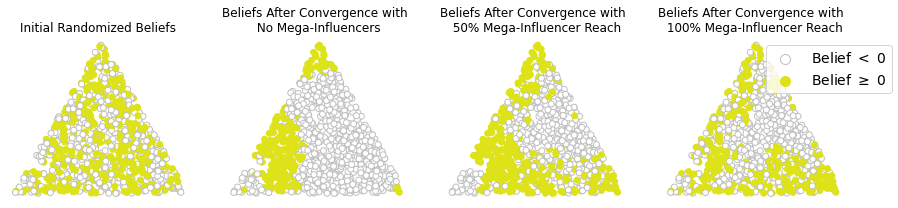
Since the onset of the Covid-19 pandemic, the extent of hesitancy regarding the vaccine has been tracked at both the U.S. national and county levels. For example, the Centers for Disease Control’s data portal includes a dataset that provides county level estimates for vaccine hesitancy based on data gathered in the U.S. Census Bureau’s Household Pulse Survey (CDC 2021). Carnegie Mellon University’s Delphi Group Covid-19 Trends and Impact Survey is available through a public API (Arnold et al. 2021) and estimates the extent of vaccine hesitancy at the county level, including changes from week to week. At the U.S. national level, Siegler et al. (2021) use survey data to track changes in vaccine hesitancy over time, and notably also include the proportion of people who change their beliefs, becoming either more or less hesitant over time, as shown in the far left of Figure 1. We show how our model can be parameterized to arrive at the empirical results presented in (Siegler et al. 2021), and discuss what this might mean in terms of the mechanism of belief proliferation. Moreover we demonstrate the formation of spatial clusters as seen in the far right of Figure 1. Other noteworthy work applying opinion dynamic models to mimic empirical results can be found for example in Friedkin et al. (2016) and Bovet & Grindrod (2020).

**Figure 1.** The figure on the far left shows results from a longitudinal survey on Covid-19 vaccine hesitancy (Siegler et al. 2021). The figure in the center shows a similar result from the ODyN model. The figure on the far right shows the geospatial clustering present in the ODyN model.

The paper is structured as follows. We begin by introducing the model, explaining its parameters, dynamics, and statistics. Next we describe a set of simulations that were carried out to perform model analysis. Finally, we present the results of these simulations, along with the application to Covid-19 vaccine hesitancy. All code and data relevant to this paper are distributed in the ODyN library.

Model

Directed graph encoding who influences whom

Let $N$ be a positive integer, and consider $N$ individuals. We use letters $u$ and $v$ (for "vertex"), $1 \leq u, v \leq N$, to label individuals. We will construct a random directed graph in which the individuals are the vertices, with a directed edge from individual $v$ to individual $u$ indicating that $v$ influences the opinion of $u$. We write

\[p_{uv} = \mbox{probability of a directed edge from $v$ to $u$}.\]

\[(1)\]

We do not assume symmetry: $p_{vu}$ need not be equal to $p_{uv}$.

Spatial locations

This part of our model is inspired by Bringmann et al. (2015), although several of the details are different here. We assign to individual $v$ a random spatial location $X_v$ in a polygonal domain $D$ in the plane. In the code available through ODyN, $D$ is assumed to be a union of triangles, and the number of individuals per triangle is taken to be random with Poisson distribution, with a rate that can be different for different triangles. The locations of individuals within each triangle are then assumed to be independent and random with uniform distribution (see Figure 2 for an example). We use triangles because they are a flexible way of approximating more complicated shapes, and it is straightforward to generate uniformly distributed random points in a triangle.

In the simulations presented here, we simply take $D$ to be a single triangle, fix $n$, and let the locations $X_1$, $X_2$, $\ldots$, $X_n$ of the individuals be independent, uniformly distributed points in $D$. We assume that $p_{uv}$ is a decreasing function of the Euclidean distance $\| X_u - X_v \|$.

**Figure 2.** In the triangle above, 1000 agents are placed in an equilateral triangle. Agents are denoted by circles, where the radius of a circle is a function of the weight of the individual agent and weights are assigned at random with power law exponent 1.5. Agents are randomly assigned beliefs from a 1-dimensional Gaussian mixture model with centers at -1 and 1, both with standard deviation 0.5. The inset square gives a zoomed in view of one section of the triangle. Directed edges are then assigned with a probability given by Equation 4, although in this image the edges are shown as directionless because of resolution constraints.

Influence weights

Following Chung & Lu (2002b), we assign a random influence weight $W_v > 0$ to each $v$. This weight determines how likely others are to listen to $v$, not how much weight they assign to $v$’s opinion; the probability $p_{uv}$ is an increasing function of $W_v$.

We assume $W_v$ to be a heavy-tailed random variable that is always greater than 1. Specifically, we assume that for any $x>1$,

\[ P(W_v>x) = \frac{1}{x^{\gamma}}\]

\[(2)\]

with some exponent $\gamma>0$. The parameter $\beta$ of (Chung & Lu 2002b) is $\gamma+1$. To generate a random number $W_v$ with the complementary distribution function (Equation 2), draw a uniformly distributed random number $U \in (0,1)$, then set

\[W_v = U^{-\frac{1}{\gamma}}\]

\[(3)\]

We will choose a value of $\gamma$ that makes the mean of the distribution of the $W_v$ finite: $\gamma>1$. Given this constraint, however, we will choose $\gamma$ to make the variance of the distribution infinite, so that outlying values of $W_v$ become fairly common. The variance is infinite for $1 < \gamma \leq 2$, and since within this range, we don’t expect the precise value of $\gamma$ to have a qualitative impact on our results, we choose $\gamma = 1.5$.

Opinion scores

Each individual $v$ carries a time-dependent opinion score $H_v$. Scores reflect the individual’s view on Covid-19 vaccines, and are centered at $-1$ and $1$, where $H_v=-1$ denotes willingness, $H_v=1$ denotes hesitancy and $H_v=0$ denotes that individual $v$ is unsure. Following Hegselmann & Krause (2002) we assume that $p_{uv}=0$ if $|H_u - H_v| \geq b$, where $b>0$ is a threshold. That is, we assume that $v$ cannot have any impact on $u$’s opinion if $u$ and $v$ have starkly different views. Throughout this paper, we fix $b=1.5$. Under this choice of $b$, the classic Hegselmann-Krause model will converge to tight consensus. However, as we will demonstrate, the ODyN model exhibits other emergent phenomena.

Overall formula for the connection probabilities

We define

\[ p_{uv} = \min \left( 1, \frac{1}{\left( 1 + \| X_u - X_v \|/\lambda \right)^\delta} ~ W_v^\alpha ~ \unicode{x1D7D9}_{|H_u-H_v| \lt b} \right)\] \[(4)\]

where $\unicode{x1D7D9}$ denotes the indicator function. The parameter $\lambda>0$ is a reference length; we take it to be the diameter of the spatial domain. The parameters $\alpha>0$ and $\delta>0$ determine the importance of influence weight and spatial proximity, respectively.

Initialization of opinion scores

The influence weights $W_u$ and spatial locations $X_u$ are independent random numbers, chosen as outlined above. We assign a random initial opinion score to each individual, drawn from a Gaussian distribution with standard deviation 0.5 and mean either $-1$ (with probability $p_{-1}$) or $+1$ (with probability $p_1 = 1 - p_{-1}$). These assignments are made independently of each other, and independently of the $X_u$ and $W_u$. The $p_k$, $k=-1,1$, are chosen to reflect publicly available data.

Opinion and network dynamics

The opinion scores $H_u$ change with time. Denote the opinion scores after $t$ time steps by $H_u(t)$. (We take $t$ to be a non-negative integer here.) Then $H_u(t)$ is the average of those $H_v(t-1)$ for which either $v=u$, or there is an arrow pointing from $v$ to $u$ at time $t-1$. In other words, $u$ averages their own opinion with the opinions of those whom $u$ is influenced by. This is the Hegselmann-Krause model (Hegselmann & Krause 2002).

Since the probabilities $p_{uv}$ depend on $H_u - H_v$, they, too, are time-dependent. The connections in the random graph are re-drawn after each time step, reflecting the fact that people don’t necessarily speak and interact with the same people every day.

In-degree and clustering coefficient

The in-degree of an individual $u$ is the number of individuals $v$ who influence $u$, that is, the number of $v$ for which there is an arrow from $v$ to $u$. We will keep track of the average in-degree. As the graph is time-dependent, so is the average in-degree. Since every outgoing arrow for one vertex is an incoming arrow for another vertex, the average in-degree equals the average out-degree.

The clustering coefficient of an individual $u$ is defined as follows. Denote by $k$ the number of individuals who influence $u$. If $k \leq 1$, then $u$ has clustering coefficient $0$. Otherwise, determine for each of the $k(k-1)$ ordered pairs of individuals who influence $u$ whether there is an arrow from the first to the second. The fraction of connected pairs is the clustering coefficient of $u$.

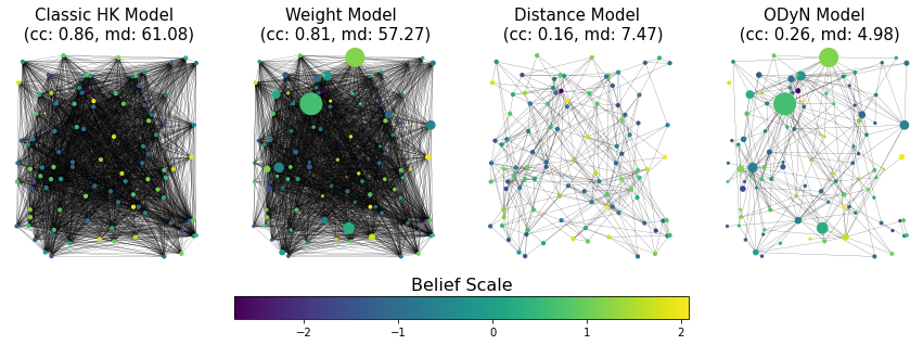
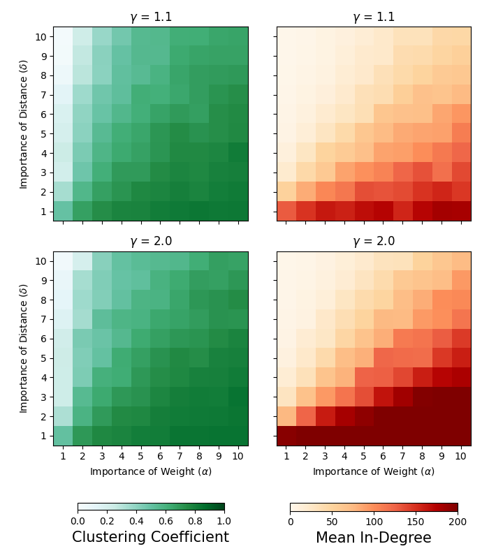
Both the average in-degree and the average clustering coefficient provide a way of evaluating whether our graphs are realistic, and therefore help us set parameters. The average in-degree should not be unrealistically high or low, and the average clustering coefficient should not be too low. To see the overall effect of varying the importance of weight and distance on the clustering coefficients and in-degree, we have performed a grid search across choices of $\alpha$ and $\delta$ with $\gamma = 1.5$, see Figure 3 (additional results for $\gamma = 1.1$ and $\gamma = 2.0$ can be found in the Appendix, Figure 9). In Figure 4 we demonstrate the effect of the inclusion of opinions, weights, and distances for a fixed choice of model parameters.

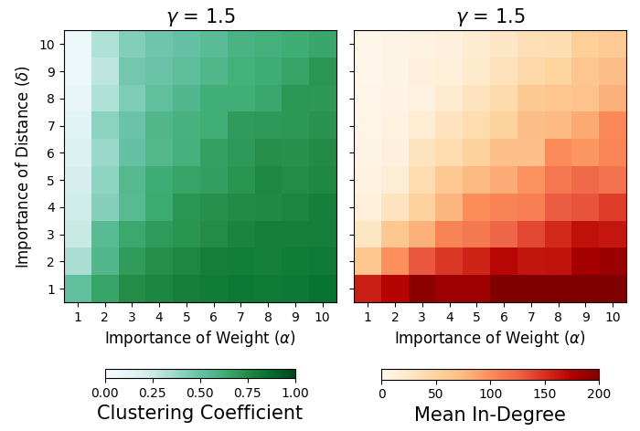
**Figure 3.** For a model with 1000 agents with $\gamma$ = 1.5 and symmetric initial beliefs centered at -1 and 1 we allow the importance of weight, $\alpha$. and the importance of distance, $\delta$, to vary between 1 and 10.

Though a person might interact with a larger number of individuals through their online social networks, or a smaller number of individuals through in-person interactions, surveys have shown that people report feeling genuinely close to between 5 and 10 individuals in their social circle, broadly construed (Dunbar 2016). In this paper we make the assumption that people will only listen to – and accept opinions from – those people who they feel genuinely close to. The clustering coefficient was chosen to be consistent with values for average clustering coefficients on directed graphs using random walks on social networks (Katzir & Hardiman 2015). Therefore in our experiments, we settle on $\alpha =2$ and $\delta = 8$.

**Figure 4.** Each of the networks above is initialized with 100 agents holding symmetric beliefs around -1 and 1. The classic Hegselmann-Krause model (left-most panel) has a very high mean in-degree (denoted md) and clustering coefficient (denoted cc). Holding all other model parameters fixed, the inclusion of weight (second from left), distance (second from right) into the full ODyN model (right-most panel) decreases the overall level of connectivity in both the mean in-degree and clustering coefficient. In models for which it is relevant, agents with greater weight are denoted by correspondingly larger dots.

Mega-influencers

We add to the model two mega-influencers, one with opinion score $-1$, referred to as the left mega-influencer, and the other with opinion score $1$, the right mega-influencer. One might think of these as modeling mass media outlets, outspoken governors, etc. To parallel similar work by Hegselmann and Krause on radicals and charismatic leaders (Hegselmann & Krause 2015), the mega-influencers hold static beliefs throughout. Recall that individual agent beliefs are initialized from Gaussian’s centered at -1 and 1, and therefore normal agents can in-fact be far more radical than the mega-influencers. The main point of the mega-influencers is to hold static beliefs that are either clearly willing or clearly unwilling.

The impact of the mega-influencers is modeled as follows. To each individual $u$, we assign two random numbers $L_u$ and $R_u$, with

\[L_u = \left\{ \begin{array}{cl} 1 & \mbox{with probability $p_L$}, \\ 0 & \mbox{otherwise}, \end{array} \right. \hskip 30pt \mbox{and} \hskip 30pt R_u = \left\{ \begin{array}{cl} 1 & \mbox{with probability $p_R$}, \\ 0 & \mbox{otherwise}, \end{array} \right.\] \[(5)\]

where $p_L$ and $p_R$ are further model parameters, with $0 \leq p_L, p_R \leq 1$. If $L_u=1$, then $u$ is susceptible to the left mega-influencer. In that case, while $H_u - (-1)< \epsilon$, where $\epsilon>0$ is another model parameter, the opinion score of the left mega-influencer, namely $-1$, will be added to the opinions over which $u$ averages in each step of the Hegselmann-Krause dynamics. Similarly, if $R_u=1$, then $u$ is susceptible to the right mega-influencer. In that case, while $1 - H_u < \epsilon$, the opinion score of the right mega-influencer, namely $1$, will be added to the opinions over which $u$ averages in each step. The parameters $b$ and $\epsilon$ play similar roles, for local interactions and for mega-influencers, respectively. In the implementation provided together with this paper, they need not be the same, but in the simulations presented here, they were the same.

Note that our model assumes that to $u$, mega-influencers do not carry more weight than friends or neighbors. The very considerable effect of mega-influencers that we will demonstrate in the computational results is all the more surprising.

Parameterization and model creation

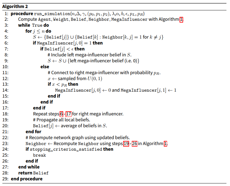
The parameters in our model are $n$, $\lambda$, $\gamma$, $\delta$, $\alpha$, $b$, $\epsilon$, $p_L$, and $p_R$. Using the ODyN library, the OpionionNetworkModel class can be initialized with these parameters as arguments. This model can be populated with individuals bearing both weight and belief scores as described in the previous sections using populate_model(). The belief propagation simulator is loaded as a separate class, NetworkSimulator, and network simulations can be carried out on the model with run_simulation(). Further documentation and demonstrations of this workflow can be found on the project Github page (https://github.com/annahaensch/ODyN), and pseudocode for these procedures are given in Algorithms 1 and 2 below.

Experimental Methodology

Model Initialization

The model described in Section 2.1 through Section 2.18 is generated by Algorithms 1 and 2 below. To populate the network, we generate uniformly distributed random points in a triangle $T$, and as our initial belief distributions, we take symmetric beliefs centered at -1 and 1 with standard deviation 0.5. We run several experiments varying the reach of mega-influencers from the left and right. Each of the experiments has $n=1000$ agents/vertices and parameters: $\lambda = 1/10$ the diameter of $T$, $\delta = 8$, $\alpha = 2$, $b = 1.5$ and $\epsilon = 1.5$. These parameters were explicitly chosen to achieve clustering coefficients and in-degrees that were realistic for real-life community interactions, namely, a consistent clustering coefficient of approximately 0.3 as well as an average in-degree around 5. As noted earlier, when generating the weights $W_u$, we used $\gamma=1.5$, which yields a heavy-tailed distribution that has finite mean but infinite variance. Our selection of parameters were chosen to mimic a real-life network in a way that’s quantitatively supported by social science research as mentioned earlier. For computational feasibility we restrict our attention to networks with only 1000 nodes, bearing in mind that such networks may be susceptible to edge effects.

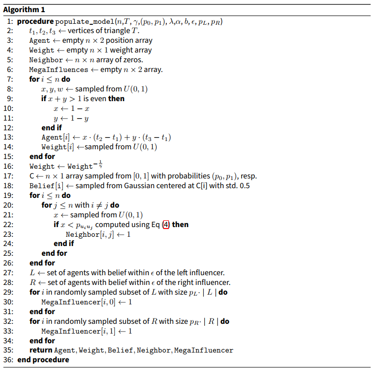
With Algorithm 1 we assign attributes to individual agents such as weight, spatial distance, position in opinion space, and connection to mega-influencers, which we then use to compute the network graph. Using Algorithm 2 we synchronously update all opinions. After each round of opinion updates, the network graph is recomputed holding weight and spatial distance parameters constant, in the manner of adaptive networks (Kozma & Barrat 2008). In the present model, this reflects the fact that somebody who influences my opinion today may not influence it tomorrow, for instance because I may happen not to talk to them tomorrow.

Stopping criterion

For each initialization and each choice of p_L and p_R, we carry out 25 experiments, using Algorithm 2. A stopping criterion is determined as follows. At each time step, a 5-time step rolling average in belief change is calculated for each individual. The community-wide mean of the absolute change in belief is then computed. When this value drops below .01, the simulation is stopped. We note that this allows for individuals to have small oscillations in opinion, but overall the community opinion stabilizes. For brevity, in Algorithm 2 we indicate this with a Boolean stopping_criterion_satisfied. This threshold is typically reached in 20 or fewer time steps.

Results

Model analysis

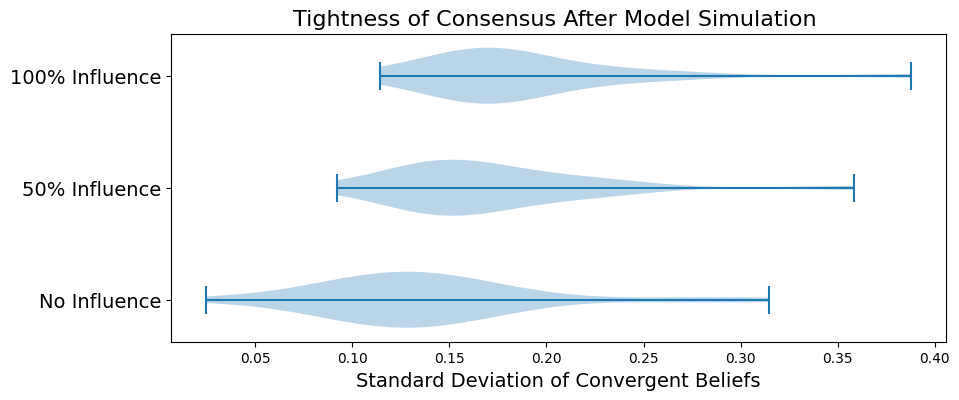
For each set of parameters, we ran 25 random seeded simulations. In Figure 5 we show how the variance of beliefs when the stopping criterion is met (see 3.3) is distributed for each set of 25 experiments. From this plot we can clearly see that a loose consensus is reached in every scenario, but always with a significantly higher variance than what is seen in a classical Hegselmann-Krause model. In the absence of mega-influencers the standard deviation of beliefs at the final time is typically around 0.13. Given 50% mega-influencer reach (i.e., $p_L = 0.5$) it is most often near 0.15 and for 100% mega-influencer (i.e., $p_R = 1$) reach it is near 0.18.

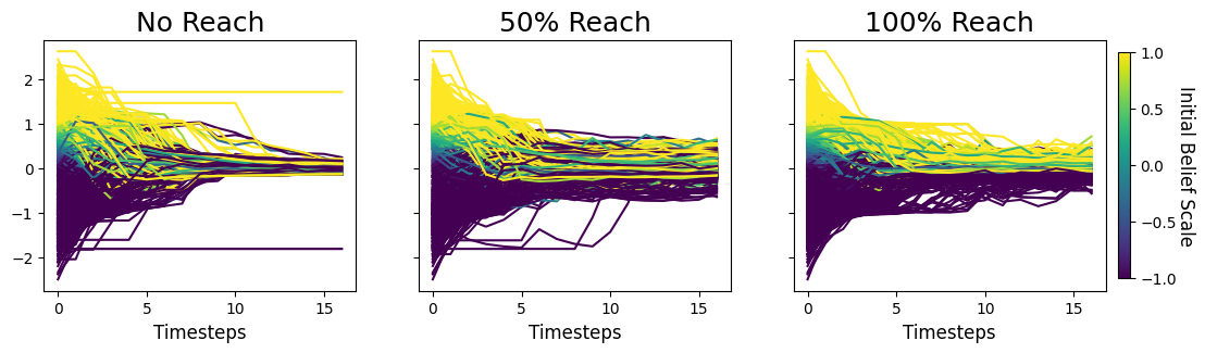
**Figure 5.** For each setting of mega influence reach (i.e. $p_R$ and $p_L$ equal to 0.0, 0.5 or 1.0) we ran 25 experiments with 1000 agents, $\alpha = 2$, $b = 1.5$, $\delta = 8$ and $\gamma = 1.5$. Here we show the distribution in the standard deviation of beliefs at the time of model convergence.

As further evidence of this behavior, we show simulation plots for one distinct iteration in Figure 6. The simulation here has reached a stopping point after 16 time steps. We observe that even in the absence of mega-influencers, agents who are situated geographically far from other agents with similar beliefs can still end up stuck in their initial beliefs and therefore become holdouts.

**Figure 6.** Sample simulation results for each setting of mega influence reach (i.e. $p_R$ and $p_L$ equal to 0.0, 0.5 or 1.0) with 1000 agents, $\alpha = 2$, $b = 1.5$, $\delta = 8$ and $\gamma = 1.5$. We see a wide spread of final beliefs as well as holdout individuals.

In Figure 7 we take a more geospatial view of the same model, and look at the beliefs as situated in space. For simplicity we color agents white if their beliefs are less than 0 and yellow if their beliefs are greater than or equal to 0. Although the relative magnitudes in each direction aren’t shown, we can confirm from Figure 6 that there is indeed a broad spread of beliefs away from 0, especially in the presence of mega-influencers. We observe that despite randomly initialized beliefs, spatially close communities of like-minded agents eventually emerge. This is seen as patchy yellow neighborhoods in Figure 7.

**Figure 7.** Sample geospatial simulation results for each setting of mega influence reach (i.e., $p_R$ and $p_L$ equal to 0.0, 0.5 or 1.0) with 1000 agents, $\alpha = 2$, $b = 1.5$, $\delta = 8$ and $\gamma = 1.5$. Agents are shaded according to belief.

Application to vaccine hesitancy

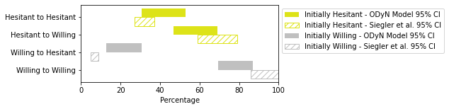
Siegler et al. (2021) present a cohort study of changes in vaccine hesitancy from a baseline survey taken between August 9 and December 8, 2020 and a follow-up survey taken March 2 to April 21, 2021. At baseline, 69% of respondents indicate that they are “likely” or “very likely” to receive the vaccine and accordingly, are classified as willing, while the remaining 31% indicate that they are “very unlikely,” “unlikely,” or “unsure” about receiving the vaccine and are therefore classified as hesitant. At the time of the follow-up survey, 47% of respondents have been vaccinated, 38% are willing to receive the vaccine but hadn’t yet done so, and 15% were hesitant. Notably, there were individuals from both initial cohorts that fell among the vaccinated, willing, and hesitant cohorts at follow-up, that is, people changed their minds to become both more willing and less willing over time. The complete data from this study can be found in the table in (Siegler et al. 2021).

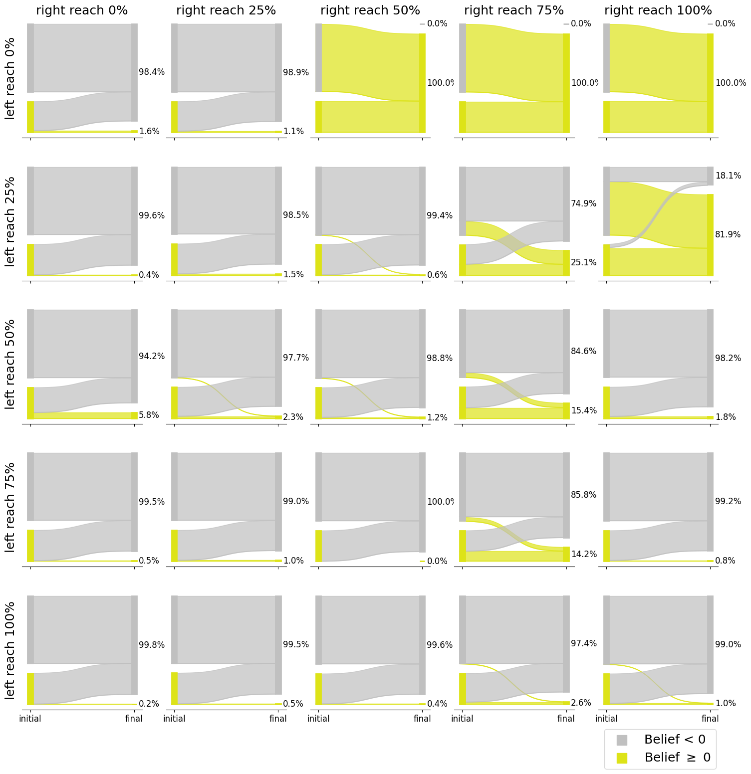
Using the ODyN model, we are able to replicate these results. We seed the model with 1000 agents and initial beliefs centered at -1 and 1 with probabilities 0.69 and 0.31 respectively, and standard deviation 0.5. Fixing model parameters $\alpha = 2$, $b= 1.5$, $\delta = 8$ we perform a grid search across different choices for left and right mega-influencer reach. The choice of parameters which best reproduced the real survey results was a left influencer reach of 35% and right influencer reach of 75%. These results were shown in the Introduction in Figure 1. For other values of $p_L$ and $p_R$, results are shown in Figure 10 of the Appendix. The plots shown in Figure 1 and 10 are for individual simulations, but in Figure 8 we demonstrate how our model compares with (Siegler et al. 2021) across multliple simulations.

**Figure 8.** The 95% confidence intervals (CI) from (Siegler et al. 2021) are shown as cross-hatched bars, and the 95% confidence intervals from 30 simulations carried out with the ODyN model ar shown as solid bars. Bars are are futher color-coded to denote whether the cohort began as Willing (i.e., Belief <0) or Hesitant (i.e., Belief $\geq$ 0). For example in the case of "Willing to Willing" our model suggests that 69% to 87% of the initially willing remained willing, whereas data from (Siegler et al. 2021) suggests that 86% to 100% of the initally willing remained willing.

Conclusion

The most interesting outcome of our model is the geospatial clustering. In particular, even an initially randomly mixed population evolves into patches of geospatially consistent beliefs. This suggests that even if there were no "blue states" and "red states" they might eventually emerge for mathematical reasons. Even individuals who are initially beyond the bounded confidence thresholds of their neighbors will eventually have their views softened.

Our model also shows the spread of opinions observed with the introduction of mega-influencers. Unlike in previous models including radicals with static beliefs, such as in Hegselmann & Krause (2015), the combination of stochasticity and mega-influencers in our model has the effect that opinions eventually stabilize, but never tightly, around a single or double consensus. Mega-influencers result in a more diffuse set of individual beliefs.

We demonstrate how a certain set of model parameters recreate real life data related to changing opinions around vaccine hesitancy. As in real life, our model shows agents changing their minds to become both more accepting and more hesitant. Of note is the fact that a substantial influence from the right is needed to prevent public opinion from almost entirely shifting towards vaccine acceptance. This is shown convincingly in Figure 10 where the presence of any reach from the left is enough to overpower all but the most broadly reaching right influencers.

Our geospatial distance can be interpreted as geographic, or some other notion of distance. Physical proximity is an important component of political and ideological opinion formation. On the other hand, social media makes spatial proximity less important, but might tend to make people interact more selectively with the like-minded as both a consequence of social and algorithmic behavioral drivers (Cinelli et al. 2021), although this is a point of discussion (Bakshy et al. 2015). One could attempt to model this effect by changing parameters in our model, making spatial proximity less important, and making like-mindedness more important, in determining the probabilities $p_{uv}$. It might also be worthwhile to consider the role of bots in networks and opinion formation online as in Keijzer & Mäs (2021).

Our results also suggest future work on the dependence on the parameters $b$ and $\epsilon$. We intend to work on scalable sampling algorithms for combining triangles into other more complex geometries. We plan to attempt to understand how time steps in our model map onto real time. Another feature to be added to the model in the future would be the effects of central interventions such as government or workplace vaccine mandates in the case of Covid-19 vaccinations. The connection between beliefs and the spread of misinformation could also be incorporated into our model.

Appendix: Additional Supporting Figures

**Figure 9.** For a model with 1000 agents with and symmetric initial beliefs centered at -1 and 1 we allow the importance of weight, $\alpha$. and the importance of distance, $\delta$, to vary between 1 and 10 with $\gamma = 1.1$ (top) and $\gamma = 2.0$ (bottom).

**Figure 10.** The model is seeded with 1000 agents, initial beliefs centered at -1 and 1 with probabilities .69 and .31, respectively, $\alpha$= 2, $b$ = 1.5, $\delta = 8$. The alluvial plot shows the overall cohort changes in belief from model initialization to the model convergence.

References

ARNOLD, T., Bien, J., Brooks, L., Colquhoun, S., Farrow, D., Grabman, J., Maynard-Zhang, P., Reinhart, A., & Tibshirani, R. (2021). covidcast: Client for Delphi’s COVIDcast Epidata API. R package version 0.4.2. Available at: https://cmu-delphi.github.io/covidcast/covidcastR/.

BAKSHY, E., Messing, S., & Adamic, L. A. (2015). Exposure to ideologically diverse news and opinion on Facebook. Science, 348(6239), 1130–1132.

BARTHÉLEMY, M. (2011). Spatial networks. Physics Reports, 499(1–3), 1–101.

BEATTY, A. L., Peyser, N. D., Butcher, X. E., Cocohoba, J. M., Lin, F., Olgin, J. E., Pletcher, M. J., & Marcus, G. M. (2021). Analysis of COVID-19 vaccine type and adverse effects following vaccination. JAMA Network Open, 4(12), e2140364–e2140364.

BEN-NAIM, E. (2005). Opinion dynamics: Rise and fall of political parties. EPL (Europhysics Letters), 69(5), 671.

BOVET, A., & Grindrod, P. (2020). The activity of the far right on Telegram. Available at: https://www.researchgate.net/publication/346968575_The_Activity_of_the_Far_Right_on_Telegram_v211.

BRINGMANN, K., Keusch, R., & Lengler, J. (2015). Sampling geometric inhomogeneous random graphs in linear time. arXiv preprint, arXiv:1511.00576. Available at: https://arxiv.org/abs/1511.00576.

CDC. (2021). Vaccine hesitancy for Covid-19: County and local estimates. Centers for Disease Control and Prevention. Available at: https://data.cdc.gov/Vaccinations/Vaccine-Hesitancy-for-COVID-19-County-and-local-es/q9mh-h2tw.

CHUNG, F., & Lu, L. (2002a). Connected components in random graphs with given expected degree sequences. Annals of Combinatorics, 6(2), 125–145.

CHUNG, F., & Lu, L. (2002b). The average distances in random graphs with given expected degrees. Proceedings of the National Academy of Sciences, 99(25), 15879–15882.

CHUNG, F., & Lu, L. (2004). The average distance in a random graph with given expected degrees. Internet Mathematics, 1(1), 91–113.

CINELLI, M., De Francisci Morales, G., Galeazzi, A., Quattrociocchi, W., & Starnini, M. (2021). The echo chamber effect on social media. Proceedings of the National Academy of Sciences, 118(9), e2023301118.

DOUVEN, I. (2019). Optimizing group learning: An evolutionary computing approach. Artificial Intelligence, 275, 235–251.

DOUVEN, I. (2022). The Art of Abduction. MIT Press.

DOUVEN, I., & Hegselmann, R. (2021). Mis- and disinformation in a bounded confidence model. Artificial Intelligence, 291, 103415.

DOUVEN, I., & Wenmackers, S. (2017). Inference to the best explanation versus Bayes’s rule in a social setting. The British Journal for the Philosophy of Science, 68(2), 535–570.

DUNBAR, R. I. (2016). Do online social media cut through the constraints that limit the size of offline social networks? Royal Society Open Science, 3(1), 150292.

FORTUNATO, S., Latora, V., Pluchino, A., & Rapisarda, A. (2005). Vector opinion dynamics in a bounded confidence consensus model. International Journal of Modern Physics C, 16(10), 1535–1551.

FRIEDKIN, N. E., Proskurnikov, A. V., Tempo, R., & Parsegov, S. E. (2016). Network science on belief system dynamics under logic constraints. Science, 354(6310), 321–326.

GARGIULO, F., & Gandica, Y. (2017). The role of homophily in the emergence of opinion controversies. Journal of Artificial Societies and Social Simulation, 20(3), 8.

HEGSELMANN, R., & Krause, U. (2002). Opinion dynamics and bounded confidence models, analysis, and simulation. Journal of Artificial Societies and Social Simulation, 5(3), 2.

HEGSELMANN, R., & Krause, U. (2015). Opinion dynamics under the influence of radical groups, charismatic leaders, and other constant signals: A simple unifying model. Networks & Heterogeneous Media, 10(3), 477.

KATZIR, L., & Hardiman, S. J. (2015). Estimating clustering coefficients and size of social networks via random walk. ACM Transactions on the Web (TWEB), 9(4), 1–20.

KEIJZER, M. A., & Mäs, M. (2021). The strength of weak bots. Online Social Networks and Media, 21, 100106.

KOZMA, B., & Barrat, A. (2008). Consensus formation on adaptive networks. Physical Review E, 77(1), 016102.

LENGYEL, B., Varga, A., Ságvári, B., Jakobi, Á., & Kertész, J. (2015). Geographies of an online social network. PloS ONE, 10(9), e0137248.

LORENZ, J. (2007). Continuous opinion dynamics under bounded confidence: A survey. International Journal of Modern Physics C, 18(12), 1819–1838.

MASTROENI, L., Vellucci, P., & Naldi, M. (2019). Agent-Based models for opinion formation: A bibliographic survey. IEEE Access, 99, 1.

MATTHIAS, J. D., Huet, S., & Deffuant, G. (2016). Bounded confidence model with fixed uncertainties and extremists: The opinions can keep fluctuating indefinitely. Journal of Artificial Societies and Social Simulation, 19(1), 6.

MURTHY, B. P., Sterrett, N., Weller, D., Zell, E., Reynolds, L., Toblin, R. L., Murthy, N., Kriss, J., Rose, C., Cadwell, B., Wang, A., Ritchey, M. D., Gibbs-Scharf, L., Qualters, J. R., Shaw, L., Brookmeyer, K. A., Clayton, H., Eke, P., Adams, L., Zajac, J., Patel, A., Fox, K., Williams, C., Stokley, S., Flores, S., Barbour, K. E. & Harris, L. Q. (2021). Disparities in COVID-19 vaccination coverage between urban and rural counties - United States, December 14, 2020 - April 10, 2021. Morbidity and Mortality Weekly Report, 70(20), 759.

PROSKURNIKOV, A. V., & Tempo, R. (2018). A tutorial on modeling and analysis of dynamic social networks. Part II. Annual Reviews in Control, 45, 166–190.

RABB, N., Cowen, L., de Ruiter, J. P., & Scheutz, M. (2022). Cognitive cascades: How to model (and potentially counter) the spread of fake news. PloS ONE, 17(1), e0261811.

ROSENSTOCK, S., Bruner, J., & O’Connor, C. (2017). In epistemic networks, is less really more? Philosophy of Science, 84(2), 234–252.

SIEGLER, A. J., Luisi, N., Hall, E. W., Bradley, H., Sanchez, T., Lopman, B. A., & Sullivan, P. S. (2021). Trajectory of COVID-19 vaccine hesitancy over time and association of initial vaccine hesitancy with subsequent vaccination. JAMA Network Open, 4(9), e2126882–e2126882.

SIMAS, C., & Larson, H. J. (2021). Overcoming vaccine hesitancy in low-income and middle-income regions. Nature Reviews Disease Primers, 7(1), 1–2.

SÎRBU, A., Loreto, V., Servedio, V. D. P., & Tria, F. (2017). Opinion dynamics: Models, extensions and external effects. In V. Loreto, M. Haklay, A. Hotho, V. D. P. Servedio, G. Stumme, J. Theunis, & F. Tria (Eds.), Participatory sensing, opinions and collective awareness (pp. 363–401). Springer.

URBIG, D. (2003). Attitude dynamics with limited verbalisation capabilities. Journal of Artificial Societies and Social Simulation, 6(1), 2.

VAN der Hofstad, R. (2016). Random Graphs and Complex Networks: Volume 1. Cambridge: Cambridge University Press.

WEISBUCH, G., Deffuant, G., Amblard, F., & Nadal, J. P. (2002). Meet, discuss, and segregate! Complexity, 7(3), 55–63.

ZOLLMAN, K. J. S. (2007). The communication structure of epistemic communities. Philosophy of Science, 74(5), 574–587.