Inverse Generative Social Science: Backward to the Future

New York University, United States
Journal of Artificial
Societies and Social Simulation 26 (2) 9
<https://www.jasss.org/26/2/9.html>
DOI: 10.18564/jasss.5083
Received: 21-Nov-2022 Accepted: 17-Mar-2023 Published: 31-Mar-2023
Abstract
The agent-based model is the principal scientific instrument of generative social science. Typically, we design completed agents—fully endowed with rules and parameters—to grow macroscopic target patterns from the bottom up. Inverse generative science (iGSS) stands this approach on its head: Rather than handcrafting completed agents to grow a target—the forward problem—we start with the macro-target and evolve micro-agents that generate it, stipulating only primitive agent-rule constituents and permissible combinators. Rather than specific agents as designed inputs, we are interested in agents—indeed, families of agents—as evolved outputs. This is the backward problem and tools from Evolutionary Computing can help us solve it. In this overarching essay of the current JASSS Special Section, Part 1 discusses the motivation for iGSS. Part 2 discusses its goals, as distinct from other approaches. Part 3 discusses how to do it concretely, previewing the five iGSS applications that follow. Part 4 discusses several foundational issues for agent-based modeling and economics. Part 5 proposes a central future application of iGSS: to evolve explicit formal alternatives to the Rational Actor, with Agent_Zero as one possible point of evolutionary departure. Conclusions and future research directions are offered in Part 6. Looking ‘backward to the future,’ I also include, as Appendices, a pair of 1992 memoranda to the then President of the Santa Fe Institute on the forward (growing artificial societies from the bottom up) and backward (iGSS) problems.Part I. Motivation
This essay is the overarching – one might say “Manifesto”– article for the present Inverse Generative Social Science (iGSS) Special Section of JASSS.1 I call this approach Inverse Generative Social Science because (a) I am interested in explaining social phenomena (b) I have a specific generative notion of explanation in mind, and (c) inverse computational methods, notably Evolutionary Computing,2 can produce agents meeting that explanatory standard. Importantly, iGSS does not change the generative explanatory standard. It offers a powerful way to evolve agents meeting it.3
From intelligent agent design to the blind model maker
To date, the agent-based modeling enterprise has consisted largely in the direct “intelligent design” of individual software agents intended to collectively generate social phenomena of interest, from the bottom up. This intelligent design programme has advanced very dramatically over the last several decades, with notable—in some cases transformative–impact on a remarkable range of fields, including epidemiology, violence, archaeology, economics, urban dynamics, demography, ecology, and environmental adaptation, on scales ranging from the cellular to the literally planetary.4 This practice of design will, and unquestionably should, continue.
Here, we explore standing this ‘paradigm’5 on its head: Rather than handcrafting completed agents to grow a given target—the forward problem—we wish to start with the macro-target and evolve micro-agents—families of them—that generate it “from the bottom up.” Rather than agents as designed inputs, we are interested in agents as evolved outputs. This is the backward problem and tools from Artificial Intelligence can help us solve it. That could be transformative 6. Several distinctions are crucial to clarify the goals of iGSS, at least as I have come to see them since my earlier articulations of this idea.
Two back-to-the-future memoranda
The first of these was in a September 1992 memo to the then President of the Santa Fe Institute, Ed Knapp, which I attach as an Appendix of possible interest. The memo was entitled Using Genetic Algorithms to Grow Artificial Societies and it gives, rudimentarily, the iGSS steps elaborated below and illustrated by the models in this collection.7
That memo refers to an earlier, August 1992, memo entitled Artificial Social Life that proposed the extension of ALife approaches to the forward problem of growing artificial societies as a whole. It suggested several lines of future research, some of which were expanded and developed with Robert Axtell in the Sugarscape work.
Organization of the paper
Although wrapped in (but hopefully not obscured by) broader themes, I will discuss (a) the aims of iGSS, (b) the steps in doing it, (c) several concrete applications, (d) foundational challenges, and (e) a central topic for the future, evolving formal alternatives to the rational actor model. That is the trunk of the essay, though there are several branches. More specifically, Part 2 updates and extends the generative explanatory standard, pointing out several important distinctions and common confusions. Part 3 discusses concrete steps in doing iGSS, with examples drawn from the four articles following this essay. Having discussed what it is (and is not) and how to do it, Part 4 discusses several foundational challenges, some shared by Economics, and highlights the specific need to develop formal alternatives to the rational actor. Part 5 discusses Agent_Zero as one such candidate. My own thinking about Agent_Zero has itself evolved since its original publication. I now give two precise senses in which this agent differs from the rational actor. Also new is a demonstration of Agent_Zero’s self-awareness that his own (here destructive) behavior lacks evidentiary basis. These points require a concise demonstration of Agent_Zero in action. For this reason only, one is presented. Also discussed are differences between Agent_Zero and some of the Dual Process (e.g., System 1 / System 2) literature, with overall Conclusions in Part 6.
This essay, then, is far more than a technical exegesis of iGSS, but tries to locate it in the broader intellectual landscape including AI, economics, rational choice theory, dual process cognitive psychology, and core issues for agent-based (and mathematical) social science as a whole.
One theme is philosophical. Einstein said, "Science without epistemology is—insofar as it is thinkable at all—primitive and muddled." Let us begin there.
Part II. Generative Epistemology and Core Distinctions
Generative explanation
Epistemologically, the defining feature of generative social science is its explanatory standard. Since iGSS adopts the same standard, it is worth clarifying it in some detail before presenting examples in Part 3.
Since the success of a model obviously depends on its goals, of which many are possible (Axtell 2016; Edmonds et al. 2019; Epstein 2008), we distinguish explanation as a general goal from others with which it is often confused. The most important of these is prediction. The distinction between explaining and predicting is central to the philosophy of science and the literature surrounding it is both extensive and complex. While there may never be a “last word” on the subject, as a first word, the explain-predict distinction is sometimes introduced by saying that predictions are claims that or when some event will occur,8 while explanations concern why, that is, by what mechanism, such events occur. Arguably, one could predict without explaining and vice versa, as argued in Suppes (1985) “Explaining the unpredictable.”9 Our focus here is on explanation, and in the case of human social systems, we have a specific, generative, explanatory notion in mind: “To explain a social pattern…one must show how the pattern could emerge on time scales of interest to humans in a population of cognitively plausible agents.” (Epstein & Chelen 2016).
Toward cognitively plausible agents
While this phrase, “cognitively plausible” is obviously open to interpretation, few would deny that a wide range of human behaviors involve (a) emotional drives, which are not necessarily conscious or “chosen” (b) deliberations, which are conscious but are bounded by incomplete information, cognitive biases, and computational/mathematical limits, and finally (c) social influence.
If one must choose a minimal set of basis elements for a space of cognitively plausible agents, these three “axes”—emotion, bounded deliberation, and social influence—have some claim to primacy, as argued elsewhere (Epstein 2013; Epstein & Chelen 2016).
One simple provisional candidate in the “span” of that minimal basis and grounded in cognitive neuroscience, is Agent_Zero (2013). This theoretical entity is offered as a simple, but formal mathematical alternative to the rational actor, in several senses discussed in Part 5 below, where a concrete example of Agent_Zero in action (in the context of violence) is given. Obviously, not all situations engage all three (emotional, deliberative, and social) of Agent_Zero’s “triple process” modules. However, in charged settings like financial panics, pandemics, or civil violence, all three modules are active, and they interact.
From bounded- to ortho-rationality
The requirement for cognitive plausibility extends earlier renditions of the generative explanatory standard. In Epstein & Axtell (1996) and Epstein (1999), Epstein (2006), bounded rationality (Simon 1972), was the sole cognitive requirement.10 I took that term to mean that in making conscious decisions, agents are hobbled by incomplete information and computational/mathematical limits. However, there was no insistence on an explicit non-conscious affective component in addition. More recently (Epstein 2013) I have argued, along with many cognitive scientists (Slovic 2010) that in diverse settings, this is indispensable. In a crude and provisional way, I included an affective (fear learning) module in Agent_Zero. Network effects aside, Agent Zero’s actions depend on her affective and deliberative modules.11 I would now say that Agent_Zero’s deliberative module is boundedly rational, but that the affective module is a-rational, or perhaps ortho-rational.12
As noted earlier (Epstein 1999) the term “generative” was inspired by Chomsky (1965). By whatever name, this notion of explanation is distinct from several others, which we now discuss.
Distinct from Nash Equilibrium
Game Theory can of course be interpreted as the pure mathematical study of optimal behavior in strategic settings. Interpreted so, it is a deep area of mathematics that does not purport to explain or predict human behavior. By contrast, for many applied game theorists (e.g., studying competition, conflict, cooperation), to “explain” a pattern is precisely to furnish a Game in which the target pattern (a set of strategies) is shown to be the Nash Equilibrium:13 If placed in the pattern, no rational (payoff-maximizing) agent would unilaterally depart from it. Missing is any mechanism whereby cognitively plausible agents (untrained and deductively challenged humans) get into the pattern, or get out of it (if dominated by other Nash equilibria14), for that matter, or how long either process might take.
Obviously, the Nash equilibrium state (e.g., mutual defection in the one-shot Prisoners’ Dilemma game) might be attained in myriad ways, including at random. The issue is whether, from its payoff matrix (expressing the strategic setting), cognitively plausible agents can attain equilibrium (deduce the optimal strategy) by reasoning. The experimental literature suggests otherwise (see Capraro et al. 2014). A memorable counter-example is an experiment conducted by Merrill Flood and Melvin Dresher at the Rand Corporation (Flood 1958). It involved an extension of one-shot play to a sequence of one-shot PD games played 100 times by Rand mathematicians Armen Alchien and John Williams, then chair of Rand’s mathematics department. The players knew that exactly 100 games would be played. By backward induction, the optimal strategy (the Nash solution) is to defect in all games.15 This is not what the mathematicians did, playing cooperate respectively in 68% and 78% of the games. When Nash himself was told of this outcome, he was surprised at “how inefficient” they were, adding, “One would have thought them more rational.” (recounted in Hodgson (2013)).
On the Bayes-Nash extension, Varian (2014 p. 281) writes, “The idea of the Bayes-Nash equilibrium is an ingenious one, but perhaps too ingenious…there is considerable doubt about whether real players are able to make the necessary calculations.”16 Of course, if the target social pattern of interest is not an equilibrium at all, then perforce, it is not a Nash equilibrium either.
So, demonstrating that an observed strategic configuration is the Nash equilibrium of a Game does not constitute a generative explanation of it (or, as Nash lamented, a reliable predictor of behavior).
Distinct from Becker optimal control
We also depart from the related Becker17 tradition in which behaviors are taken to be explained when they are demonstrated to be solutions (extremals) of an optimal control or dynamic programming problem, as in Becker & Murphy's (1988) famous article, “A Rational Theory of Addiction.” As with the vastly simpler problem of maximizing a standard (e.g., Cobb-Douglas) utility function subject to a budget constraint, solving–indeed, even formulating–such mathematical problems vastly exceeds the cognitive capacity of untrained humans.
Therefore, if the Becker School’s contention is that humans are setting up and solving such optimization problems, it is prima facia untenable, and is rejected by many economists, including Akerlof & Shiller (2010), and of course by Keynes (1936), who famously wrote:
Most, probably, of our decisions to do something positive18, the full consequences of which will be drawn out over many days to come, can only be taken as a result of animal spirits — of a spontaneous urge to action rather than inaction, and not as the outcome of a weighted average of quantitative benefits multiplied by quantitative probabilities.
More importantly, the assumption of optimization flies in the face of extensive empirical counter-evidence from cognitive psychology and behavioral economics (e.g., Simon 1972; Allais 1953; Ariely 2008; Dawes 2001; Ellsberg 1961; Kahneman et al. 1982; Kahneman 2011; Slovic 2010)19.
Friedman’s gambit declined
Friedman's (1953) famous "Positive Economics" gambit was to (a) grant this point, (b) deny imputing such powers to humans, and (c) claim that people and other economic actors (e.g., firms) behave simply “as if” they were optimizing.20 Because otherwise, they are selected out.21 This is quite inconvenient for the Becker-Murphy addiction model since what they claim to be rational behavior (namely addiction) increases the risk of being selected out, by overdoses!
More pertinent, are we to say that freely falling rocks are acting “as if” they were solving Newton’s equations? “Conforming to” the equations and “solving” them strike me as radically different. While it is untenable that we humans are formulating and solving Bellman’s equations (or applying Pontryagin’s maximum principle), it is clear that in many natural and experimental settings, we are not even conforming to them.22
Furthermore, since one could also arrive at an optimum by random walk or imitation, are Friedmanites not compelled to say the actors of interest are also behaving “as if random” and “as if imitating” and “as if” any of the innumerable processes that could eventually arrive at an optimum"? If so, why retain the word “rational” at all, since, on the “as if anything” reading, it is devoid of any specific cognitive content, as its proponents curiously insist. As for Becker and Murphy, rather than “a rational theory of addiction,” perhaps what they truly displayed was an irrational addiction to theory!
In any event, neither Becker nor Friedman (nor their lineage) appear interested in generating observed macro-social phenomena from the bottom up in populations of cognitively23 plausible (and perforce heterogeneous) agents, a notion we will clarify below in connection with Rational Choice Theory and the Agent_Zero approach.
Distinct from macroeconomic regression
Another approach that—while very powerful—is not explanatory in our generative sense is aggregate regression. Regression may well predict the response of an aggregate dependent variable to changes in one or more aggregate independent variables. This, however, gives a purely macro-to-macro account when we want a micro-to-macro account. To a generative social scientist, the aggregate relation (the regression equation) itself is the explanandum. That is the target we wish to grow! When agent modelers give a bottom up generative account of some macro pattern, they are sometimes challenged with the question, “Couldn’t you just do that with a regression?” The answer is "No, you couldn’t do that—give a micro-to-macro account—because the micro world is absent from the regression.
Distinct from compartmental differential equations
Likewise, in epidemiology a well-mixed compartmental differential equation epidemic model may well produce the same population-level infection curve as an ABM (Rahmandad & Sterman 2008). However, the former does not illuminate how that macro pattern could emerge from a population of cognitively plausible interacting agents. The model outputs (the aggregate curves of cases over time) are the same, but the agent-level generative mechanism is absent from the classical compartmental differential equations.
Generative explanation for policy
If we care solely about aggregate prediction, we may not need the micro-mechanism. However, if we wish to design interventions at the micro-level of agent information, expectations, and rules, a representation of the micro-world is essential. What changes to the micro rules will induce—from the bottom up—a different ‘emergent’ macroscopic pattern, like a more healthy, peaceful, or equitable society? In the COVID-19 pandemic, epidemiologists used differential equations to estimate the vaccination level required to produce herd immunity at the population (macro) scale. The problem was how to induce that level of vaccine acceptance by large numbers of misinformed and unduly fearful individuals at the micro scale. In such cases, explanation—understanding cognitive micro mechanisms—may be more important for the design of policies and policy messages than mere macro-scale prediction.
Posit vs. Generate
Another important distinction that I have encountered is between positing and generating. To some, the motto of generative social science is “If you didn’t grow it, you didn’t explain it” (Epstein, 1998). That is emphatically not a dictat that “You must grow everything in your model.” Some elements of every model must be posited. These may be very important actors, treated as agents in their own right, like intermediate institutions (e.g., the Federal Reserve). The point is purely definitional: if they aren’t generated, then they aren’t explained. That does not mean they are inessential or forbidden, much less that the model is somehow a failure if it posits non-generated elements. To insist that every element of a model be generated invites an infinite regress of demands that every generator itself be generated and it’s “turtles all the way down.”
After all, even biological evolution began with primitive constituents (the chemical elements) and rules governing their permissible combinations (the laws of Physics).24 Of course, as in Physics, we always look for more fundamental unifying laws that entail the ones in hand.25 But we don’t suspend science in the meantime.
Necessity vs Sufficiency
Centrally, the motto (‘Not grown implies not explained’) must not be confused with its converse (‘Grown implies explained’)26 as explicitly stated in several publications, including Epstein (2006 p. 53):
"If you didn’t grow it, you didn’t explain it. It is important to note that we reject the converse claim. Merely to generate is not necessarily to explain (at least not well) \(\dots\) A microspecification might generate a macroscopic pattern in a patently absurd—and hence non-explanatory—way." In sum, “generative sufficiency is a necessary but not sufficient condition for explanation.” (Emphasis in the original).
Uniqueness vs. Multiple generators
Finally, the motto does not say there is only one way to grow it. As noted in a series of publications (Epstein 1999, 2006, 2013; Epstein & Chelen 2016), there may be many ways to grow it; many agent specifications that suffice to generate the target, be it segregation, or the skewed distribution of wealth. That is precisely the point of iGSS: to enlist AI approaches in the discovery or evolution of multiple generators.27
Adjudication between competing generators
It is an embarrassment of riches, not an embarrassment, to have multiple generators. As in any other science where theories compete, we must of course devise ways to adjudicate between them, by collecting new micro-data or designing new experiments at the micro-scale. As often occurs in science, new theory may precede and guide data collection and experimental design. It is no different here. Having multiple generators is also common in climate science, hurricane forecasting, and epidemiology where several mechanistically different but empirically credible models are used to form a probabilistic “cone” over possible futures. Inverse methods can provide us with families of this type.
In summary, the motto does not say that generating is sufficient for explanation; it does not say that one must generate everything in one’s model; and it does not say generators are unique. Generative sufficiency confers explanatory candidacy. If there are multiple candidates, more empirical or experimental work is required to adjudicate between them, as in every science.
Having discussed critical distinctions and goals, and having insisted on the addition of an affective (not just boundedly-rational) component in charged settings, we now present the modular Agent_Zero, as a minimal cognitively plausible agent. This sets up the Part 5 demonstration of Agent_Zero as an alternative to the rational actor and the proposal to “disassemble” Agent_Zero and evolve alternatives to it using iGSS.
The modular Agent_Zero
Agent_Zero’s observable behavior is produced by the interaction of internal affective and boundedly-rational deliberative modules28 (each an explicit real-valued function). In addition, Agent_Zero is a social animal influenced by other emotionally-driven and boundedly-rational Agent_Zeros in social networks. These networks form and dissolve endogenously based on affective homophily.29 The agents’ behavior changes their environment (a landscape of aversive stimuli, attacks in the violence illustration), which feeds back to change the agents, so micro and macro are in fact coupled. All mathematical and computational specifics of Agent_Zero are given in Epstein (2013). Importantly, however, my stated goal was “not to perfect the modules but to begin the synthesis,” and to do so formally. This is crucial.
Formalization
All but the most doctrinaire would grant that humans are not perfectly rational, but would argue that the rational actor model is a mathematically tractable and fertile abstraction like the ideal gas. As the saying goes, “You can only beat a model with another model,” and lacking a formal alternative, the rational actor will hold sway. As Kahneman writes, “Theories can survive for a long time after conclusive evidence falsifies them, and the rational-agent model certainly survived the evidence we have seen, and much other evidence as well.” (Kahneman 2011 p. 374). Albeit crude and provisional, Agent_Zero is a formal alternative.
The affective module
For the affective module of Agent_Zero, I used the classic, but very simple, Rescorla & Wagner (1972) equations of associative fear learning (given a stimulus) and extinction (when the stimulus stops). These crudely capture the performance (not the tissue science) of the amygdaloid complex in a wide range of vertebrate species including humans. Very interesting work by Trimmer et al. (2012) demonstrates why natural selection could favor the Rescorla-Wagner fear-learning rule. However, as noted in Epstein (2013) and in Epstein & Chelen (2016), there are several existing alternatives to explore,30 and an even larger family to evolve computationally from more fundamental rule primitives, as proposed below.
The deliberative and social modules
Similarly, there are many alternatives to Agent_Zero’s boundedly-rational deliberative module, which computes a moving average31 of local relative attack (aversive stimulus) frequencies over a memory window.32 The same point applies to affective homophily33 as the endogenous mechanism of network formation, making it a “triple process” model if you like.
Entanglement
Finally, I began with a linear combination of modules, when we know that these can be deeply entangled, as when our fear of an event (the emotional module) distorts our estimate of its likelihood (the deliberative module). In that case, just as Hume would have it, “Reason…is a slave to the passions.” I proposed a simple nonlinear functional form entangling these modules, without adding parameters, in which fear of an event distorts our estimate of its probability.34 This is another very fertile area to be sure.
My commitment, then, was to a formalized synthesis, not to the components (though defensible as a starting point). And from Agent_Zero’s constituents, iGSS can discover new ones, and combine them in new nonlinear ways. As I wrote of the published versions of Agent_Zero,
“Whether this particular agent, or some distant progeny yet to emerge, I believe this broad family tree of individuals—each capable of emotional learning, bounded rationality, and social connection—is well worth developing.” (Epstein 2013 p 193)
In the present context, I would say, “well worth evolving,” using evolutionary computation and other tools from AI. In several respects, however, Inverse Generative Social Science would be a new use of AI.
AI, emulation and explanation
As noted in Epstein (2019) and in our iGSS Workshop Descriptions, Artificial Intelligence is displacing humans. It is augmenting humans. It is emulating humans. It is defeating humans. It is not (yet) explaining them. We want to enlist it in the (generative) explanatory enterprise. For example, AlphaZero annihilates humans at chess. But this does not illuminate how humans play chess.
In one famous game, Gary Kasparov defeated IBM’s Deep Blue with a startling sacrifice. When asked how he came up with that brilliancy, Kasparov answered, ‘It smelled right.’ I would say that we humans do many things “by smell,” without the explicit comparison of costs and benefits assumed in textbook renditions of economic choice.
Choice-free aspects of social science
As discussed above, the evolved human fear apparatus, which generates a great deal of observable behavior, is not choice-like, or necessarily even conscious, much less “rational.”35 Yet, it exhibits dependable regularities we can represent (at least crudely) in mathematical models.
Now, a committed Rational Choice theorist would counter that the fear—even baseless fear–is subsumed in one’s utility function and that, given the fear, you then optimize your behavior. In the case of fear (and several other emotions36), this is not supported by the neuroscience.
You do not in fact optimize behavior given your fear, you often behave before you are aware of your fear. As James (1884) put it, ‘you don’t run because you fear the bear. You fear the bear because you run.’ For the contemporary neuroscience of this, see LeDoux's (2002) discussion of the “low road” (amygdala-based: fast and inaccessible to conscious ratiocination) and the “high road” (prefrontal cortex: delayed and evidence-based) of the human fear response. If a snake lands in your lap, you instantly freeze. You do not choose to freeze. Only after that do you consciously evaluate whether it is a real or a rubber snake and choose whether to remain motionless.
The central point, however, returning to AI is that defeating and displacing humans does not illuminate how humans work. The confusion is between the emulation of human output and the revelation of a human generative mechanism. Perhaps the most glaring example of this confusion is Turing’s own Imitation Game.
The Turing Test is irrelevant to explanation
Turing (1950) considered the question, “Can machines think?” to be too unclear to warrant discussion (for a challenge, see Chomsky (2009)) and proposed to replace it with (paraphrasing), ‘Can we distinguish the computer’s responses from those of a human in [his famous] Imitation Game?’ Whatever else might be gained from the Imitation Game, it is clear that a machine’s emulation of human output per se does not illuminate how (the mechanism by which) humans generate that output. How so?
Imagine the following Imitation Game. Behind Turing’s screen is a soprano and a perfect recording of that same soprano. No human subject can tell them apart. The recording tells me nothing about how humans vocalize. By what mechanism do humans generate ‘sounds?’ By blowing wind across vocal chords, whose vibrations produce travelling waves in the medium, and so forth.37 The perfect recording gives me no clue.38 As Chomsky (2009) has written,
“\(\dots\) a machine is a kind of theory, to be evaluated by the standard (and obscure) criteria to determine whether the computational procedure provides insight into the topic under investigation: the way humans understand English or play chess, for example…. Questions about computational—representational properties of the brain are interesting and seem important; and simulation might advance theoretical understanding. But success in the imitation game in itself tells us nothing about these matters.” (Emphases added).
Talking AIs
An equivalent confusion arises in connection with “Talking AIs.” That a Large Language Model (LLM) trained on massive data can spit out grammatical English word strings tells us nothing about how humans acquire a grammar in the first place, with no such training and long before they even have a notable vocabulary on which to train! The central cognitive science question is precisely how the infant acquires a grammar (a finite rule system capable of generating the infinite set of all and only grammatical word strings) given the extreme “poverty of the stimulus.” (See Berwick et al. (2011)). Indeed, how does the infant brain even distinguish—from the cacophony into which it is born–those auditory stimuli (again, waveforms in the medium) that are linguistically salient, from the ambient sounds of rustling leaves, parental sneezes, and crashing dishes? For a pellucid statement of the issue, see (S. D. Epstein & Hornstein 1999). Despite the myriad applications of LLMs, human grammar acquisition involves an innate cognitive endowment that the massively trained LLM neither possesses, formalizes, nor illuminates.39
Big data end of theory
The same general emulate-explain confusion has other incarnations, including the “End of Theory” big data movement, if I may.40 Again, either we are proposing to abandon the search for underlying generative mechanisms, or we are purporting to reveal them by vast sampling of output. The latter seems fatuous, as if ‘To understand how the steam engine works, let us begin by sampling clouds of emitted steam; collect Big Steam Data.’ Suppose we can construct a model that produces the same data. The model might even let one predict emitted Steam at time \(t + 1\) from emitted Steam at time \(t\). However, this teaches us nothing about how the steam engine works. The emulation of output does not illuminate generative mechanism.
Markov models simply encode the problem
In turn, suppose we have a cognitively plausible micro-mechanism, \(m\) that generates a macroscopic target pattern, \(M\). Some would say that \(m\) is unnecessary because \(M\) is the equilibrium distribution of some Markov Process with transition matrix \(T\). To give this position it’s due, let us think of \(M\) as a stationary distribution of wealth across social groups. It is certainly deep and interesting that (under several mathematical strictures) for any \(M\), there exists a Markov transition matrix41 \(T\) whose terminal distribution is also \(M\). How does \(T\) (a list of transition probabilities) illuminate the mechanism, \(m\)? \(T\) might predict, but it does not explain. Why is the inter-generational transition probability from poor to rich so low in America? If we want to change it by designing interventions at the micro (e.g., urban neighborhood) scale, we need more than the transition probability itself. We need mechanisms, like polluted environments, poor schools, systemic discrimination, and the ambient threat of violence.
\(T\)’s entries alone simply encode the social problem. They are the target of the ABM, not a substitute for it. Here again, explanation is essential to policy.
Having clarified some broad goals of iGSS, made some central distinctions, and situated it in the broader discussion, there are six essential steps in actually doing it in particular cases.
Part III. Concrete Steps of iGSS with Examples from the Collection
Each of the models in the present collection, and many beyond, address their topics in their own way. In some respects, these are requirements of Genetic Programming generally. Of course, one must begin with an explicit target of some sort (or there is nothing to explain). What aggregate pattern or collective functionality are we attempting to generate? Step 1, therefore, is:
- Stipulate the macro (or other) target (i.e., what you are attempting grow).
The papers in the present collection exhibit a colorful range. In Gunaratne et al. (2023), the target is a stable mixed racial residential pattern in an artificial Schelling-like segregation model. In Vu et al. (2023), it is the empirical time series’ of drinking (alcohol consumption) data for males and females in New York State from 1984 to 2016, the challenge being to simultaneously generate both time series. In the flocking and opinion dynamics models from Greig et al. (2023), it is (a) a dynamic reference pattern, from the famous Boids model (Reynolds 1987) of flocking behavior and (b) multi-modal (including polarized) opinion dynamics. In Miranda et al. (2023), it is the true performance of human subjects in a common pool resources (irrigation) experiment. Having stipulated the target output, the next task is to:
- Stipulate the agent rule-constituents, or primitives, as distinct from numerical parameters and their ranges.
Examples of agent rule constituents from the Gunaratne et al. (2023) mixed Schelling segregation model include: the agent’s preference for like-colored neighbors, the average age and racial composition of each candidate neighborhood, its distance from the agent’s current location, and the agent’s moving history. In the Greig et al. (2023) Flocking model, ‘avoid collisions,’ ‘normalize,’ and ‘maintain separation’ are primitives. In the Vu et al. (2023) alcohol model, ‘conform to the injunctive norm’ (the agent’s perception of acceptable drinking by sex) and ‘maintain drinking habit’ (based on prior drinking level) and autonomy are available rule constituents. In the Miranda et al. (2023) common pool irrigation game, upstream and downstream homophily are rule constituents.
Obviously, the initial number of agents or the agents’ maximum vision would be global variables or numerical parameters, but not agent rules. These numbers of course must also be assigned for the models to run. To evolve rules from primitives, we must
- Stipulate the permissible concatenations of primitives.
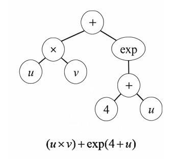
These primitives can be combined in innumerable ways to form agent rules. In most Genetic Programming since Koza (1992), the complete rule is represented as a Tree structure with primitives as terminals and permissible combinators as nodes. Edges can encode mathematical operations like addition, division, square root, or logs and also logical operators such as ‘if-then’ and ‘not.’ One can also permit or constrain the nesting of operators, as in \(log(log(x))\). In purely mathematical problems, the nodes would be variables like x and y, and the edge structure might stipulate that, for example, the log of their product should be raised to some power. The GP Tree representation of the function: \(uv + exp(4+u)\) is shown in Figure 1 (Click on graphics to enlarge).
In our cases (displayed below) the terminals are rule-primitives, like “fraction of like-colored neighbors,” “move to,” or “maintain a threshold separation distance.” The combinators include logical operators like “if-then” and “not.”
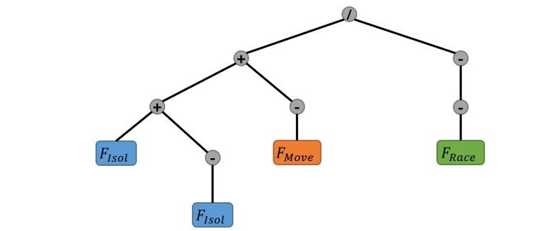
The winning Tree, or agent architecture, from Gunaratne et al. (2023) is shown below in Figure 2. Notice its retention of Schelling’s sole rule shown in green.
As in all evolutionary computing, rule trees (agent architectures) below some fitness threshold are selected out while performers above it progress to the next round of mutation, crossover, and selection.
There are two specifically evolutionary aspects of the approach. First, complete Trees can mutate (e.g., at a terminal) and can crossover (have sex with other trees) to produce offspring trees. In the (present collection) Gunaratne et al. (2023) Schelling model, the Vu et al. (2023) alcohol model, and the Greig et al. (2023) flocking and opinion dynamics models, crossover is used. In the Miranda et al. (2023) irrigation model, it is not. To bound the search space of Trees (rules), one can also impose limits on their complexity, variously defined (e.g., expression length, logical depth), which is done in several of the models.
Agents scoring well on one fitness metric may score poorly on another, so the choice of fitness metric will channel the evolutionary process, bringing us to the fourth step:
- Stipulate a fitness metric.
When we run an ABM, we are mapping (sending an element of) a domain space of micro-scale agent architectures to an image-space of macroscopic patterns or collective functionalities. Some member of the latter set is the Target. The fitness of an agent model (micro-scale) is the proximity of its generated output to the target (macro-scale).
The evaluation of fitness therefore requires that we metrize the set of macro-patterns and compute the distance between the model-generated macro-pattern and target macro-pattern. This is done in many modeling areas and can typically be done in many ways. For positive integer values of \(p\), the \(L_{p}\) norms used to compute the distance42 between two functions (one the target and one the model output) are themselves countably infinite. In the earlier Artificial Anasazi modeling (Axtell et al. 2002) we explicitly offered goodness-of-fit (i.e., model fitness) on three of these \(L_{p}\)-norms. In no way is this Step a distinctive challenge for ABMs (or inverse ABMs), then.
In the present collection, Greig et al (2023) use the mean-squared error (MSE) with respect to the target flocking and opinion patterns, while Miranda et al (2023) use 1-MSE in their irrigation model. Vu et al (2023), use the implausibility metric from Approximate Bayesian Computation (ABC) as in Andrianakis et al. (2015).
Importantly, one can include a complexity penalty in the fitness function itself, to bias selection toward human-interpretable models.43 A simple such penalty is the number of nodes in the tree representation of the agent. Vu et al. (2019) put an upper limit of 16 elements on the set of evolved agent rules, for example. The next step is to
- Stipulate an evolutionary algorithm.
To ensure replicability, one must explicitly state the algorithm used to evolve agent architectures. The present collection exploits several of these: Gunaratne’s Evolutionary Model Discovery (EMD) engine is completely open source and is used in the Schelling extensions published here, in the earlier, very interesting extensions of the Artificial Anasazi model in Gunaratne & Garibay (2020), and in the collective action irrigation model of Miranda et al. (2023). The DSL tool is employed by Greig et al. (2023), and the Grammatical Evolution engine is used by Vu et al. (2023). Google has released a Genetic Programming engine as well, and several ABM environments include them. Finally, we must
- Stipulate a stopping rule.
Only in rare cases can we say definitively that the GP has found the absolute global peak of a typically rugged fitness landscape.44 Therefore, we must furnish the GP with a stopping rule, which could be a time limit, a “satisficing” fitness threshold, or other criterion. In this collection, a finite generation count is used in all but the Greig et al model, which uses a loss threshold as its stopping rule.
An interesting possibility is that, when the stopping rule is applied, the winning architectures may retain functionless “Darwinian tubercles”45 that evolution (the GP) “never got around” to eliminating.
Table 1 gives all these six elements for each of the four articles (five models) below.
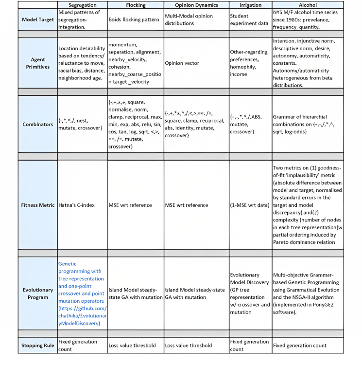
The new locus of design and architecture
As the Table makes clear, iGSS does not dispense with intelligent design. Rather, it changes the locus of design from the completed agent to more elemental building blocks for the computational evolution of agent architectures. Architectures become specific agents when numerical parameter values and initial conditions are assigned. Architectures, then, are truly distinguished by the agents’ rules.
Rules are natural language expressions
Centrally, when we speak of agent rules in an architecture, we have in mind natural language expressions, not numerical parameters. The distinction between parameters and rules is crucial for two reasons. First, we know how to measure the distance between two real number parameter values. We, I will argue, do not know how to (usefully) measure the distance between two rules. This is problematic (and not just for agent modeling) in connection with model sensitivity to rule perturbations. Second, agent rules can in principle be written out longhand in English46 (or English pseudo-code) which will be useful in considering the tradeoff between accuracy and human comprehensibility. In some cases, the tradeoff is steep. Surprisingly, in others, the fittest evolved rule can be remarkably simple.
Rule fitness vs. Interpretability
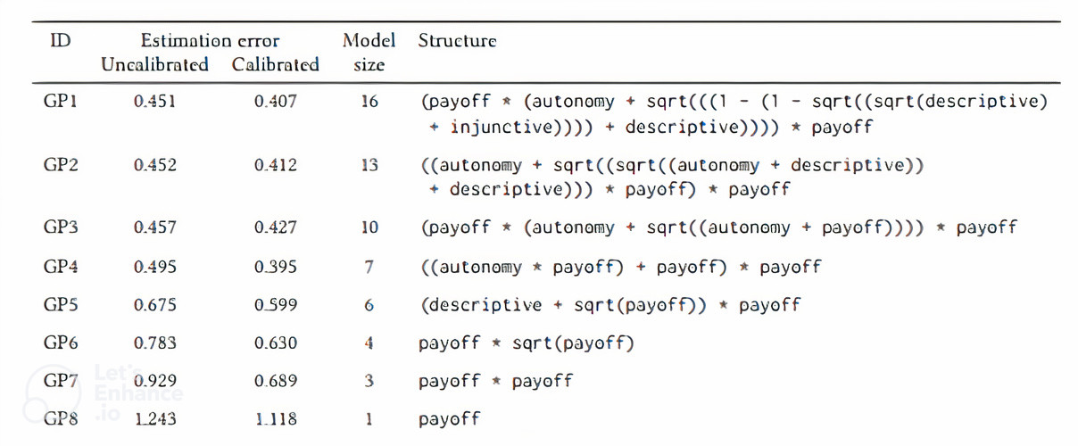
An earlier published example of a steep accuracy-comprehensibility tradeoff is below, from Probst et al. (2020). There, we used iGSS to discover rules of drinking behavior that generate the true alcohol consumption time series data for NY state over the period 1984 to 2020. The four primitives were payoff (hedonic satisfaction), the injunctive norm (appraised opprobrium associated with drinking), autonomy, and the disjunctive norm (the agent’s appraisal of drinking prevalence. Permissible concatenations were \(\{+, -, *, \sqrt\}\) with nesting (recursion) of expressions permitted. Table 2 gives the final fitness ranking of the top eight evolved agent rules.
The tradeoff between rule fitness and complexity is shown in Figure 3.
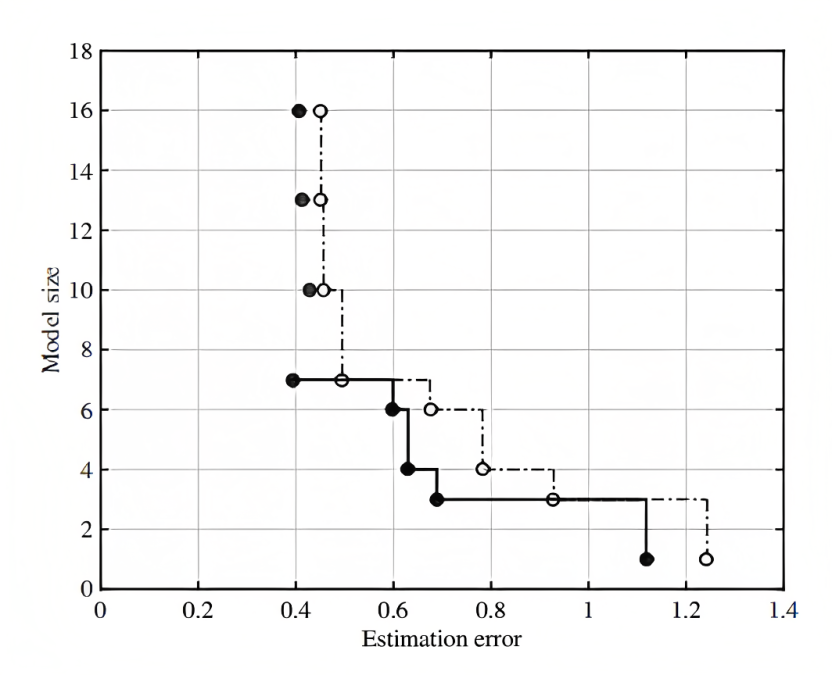
In this case, the tradeoff between empirical fit and human comprehensibility (or perhaps, the likelihood of human design) is clear. GPs 1 through 8 are agent rules evolved by the Genetic Program. In Table 2, the fittest rule, GP1, is the most complex, involving triply-nested square roots of primitives. The least complex GP8 is the simplest and most interpretable, but also the least fit. In gauging the likelihood that a human would have handcrafted a successful generative rule, the English language (or pseudo-code) rendition is very useful.
Conserved elements and rule phyla
This set of GPs also exhibits building blocks that are conserved across algorithmic evolution.47 While the use of payoff only has lowest fitness, it is conserved as the primitives autonomy, descriptive norm, and injunctive norm are successively added by evolution producing ever-fitter agent architectures.48 We might define phyla of architectures by such conserved elements. Different designed starting points—parent trees–will propagate different agent phylogenies. Below we discuss the difficulties of defining mathematically proper neighborhoods of rules. Phyla of rules, however, pose no such problems. In Figures 6 above and 7 below, from Gunaratne et al. (2023), we see that Schelling’s single factor (racial preference) was retained as a tree node (colored green) in several more complex evolved architectures.
Punctuated equilibrium
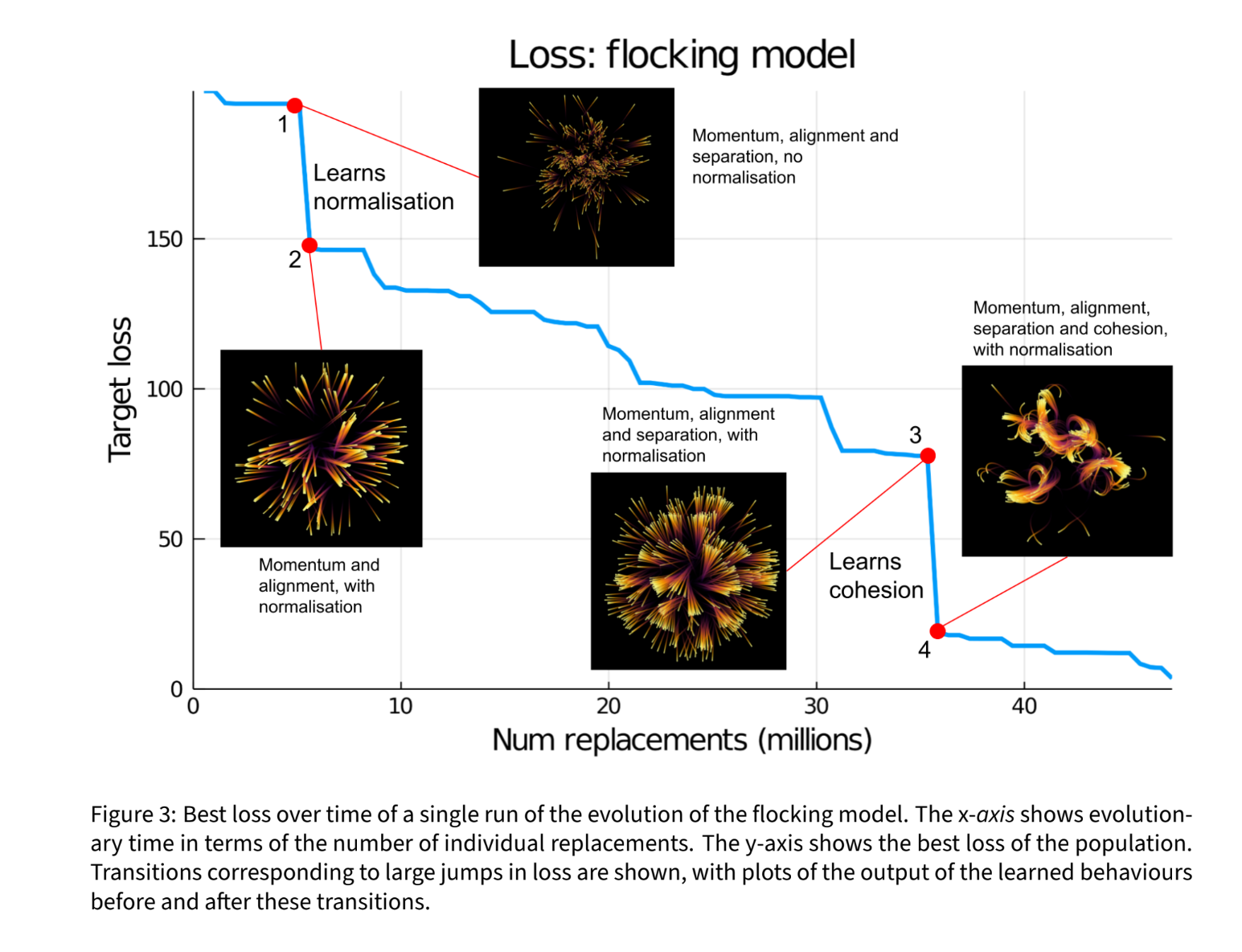
The retention of conserved rule elements (primitives), with successive abrupt evolved improvements, or “jumps,” can lead to so-called punctuated equilibrium (Gould & Eldredge 1972). This is illustrated in Figure 4 from Greig et al. (2023). Here, the agents first learn momentum, alignment, and separation. Then they “discover,” and add, normalization, followed by cohesion, producing a stepwise (not “gradualist”) evolutionary trajectory ending in the target phenomenon, flocking.
A different punctuated learning trajectory was found in the drinking model of Vu et al. (2023), as shown in Figure 5.
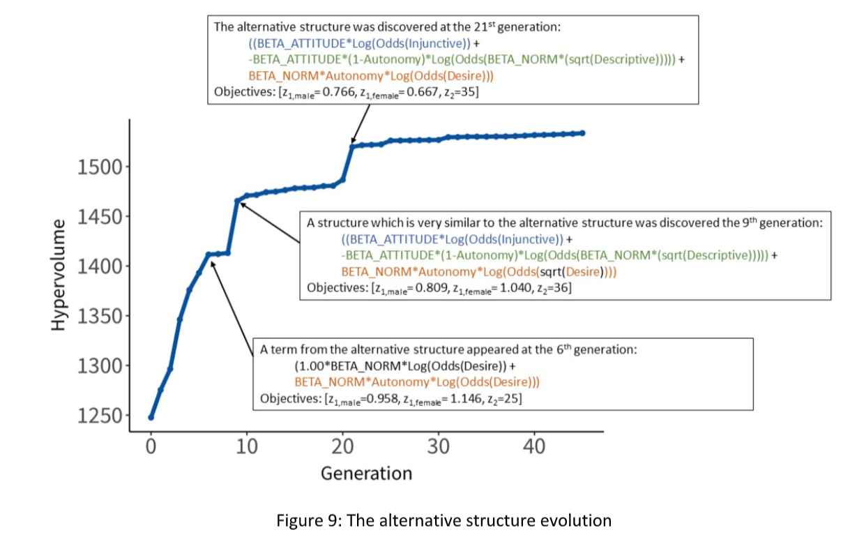
Notable are the waiting (searching) times between the successive (punctuated) equilibria (horizontal segments). They appear at generations 6, 9, and 21, as shown in Figure 5.
iGSS and calibration
Because it starts with an explicit Target (empirical or artificial) iGSS is automatically aimed at calibration. That is, the fitness function is precisely the proximity of the model’s output to the target, so agents (rules plus parameters) that are too poorly calibrated (that is, fit) are selected out. High fitness means good calibration.
What we obtain from the inverse generative exercise is, in the best case, a family of well-calibrated ABMs. In this regard, iGSS shifts the empirical burden to adjudicating between the auto-calibrated generators, on grounds of comparative cognitive plausibility at the individual agent level.49
Emergent simplicity: The inverse mixed Schelling model
We have seen that the fittest evolved Rules can be the most complex. But the reverse may obtain, as we discovered in the inverse Schelling model of Gunaratne et al. (2023). Schelling’s original model contained only one primitive: the preferred fraction of neighbors of one’s own race. Famously, even when agents do not insist that a majority of neighbors (as few as 1 in 4 neighbors) share their color, segregation results. Because we were interested in generating mixed, not segregated, neighborhoods, Gunaratne et al. (2023) expanded the primitives beyond race alone, which is retained as an available constituent. For any neighborhood, \(i\), the Schelling primitive (the fraction \(F\) of racial similarity) is denoted \(F_{Race}(i)\). The new primitives are: mean neighborhood age \(F_{Age}(i)\); distance from present home location \(F_{Dist}(i)\); the agent’s preference for isolation \(F_{Isol}(i)\); the agent’s tendency to move \(F_{Move}(i)\), based on movement history, and \(F_{Neigh}(i)\), the mean utility (“satisfaction”) of the candidate neighborhood’s residents. Permissible combinators were given above in Table 1. Notably, ratios and products (and, by iteration, powers) of terms are permitted, allowing highly nonlinear rules. The top ten evolved rules are given in Table 3. Note that these are not simply weighted linear combinations.
| Rule | Mean c-Index |
|---|---|
| \(u_{a,i}=-\frac{F_{Move}(a,i)}{F_{Race}(a,i)}\) | \(0.3047\) |
| \(u_{a,i}=-\frac{F_{Race}(a,i)}{F_{Isol}(a,i)} - F_{Isol}(a,i) - 2\frac{F_{Age}(a,i)F_{Isol}(a,i)^2}{F_{Race}(a,i)F_{Dist}(a,i)}\) | \(0.2260\) |
| \(u_{a,i}=-\frac{F_{Race}(a,i)}{F_{Isol}(a,i)} - F_{Isol}(a,i) - \frac{F_{Age}(a,i)F_{Isol}(a,i)}{F_{Race}(a,i)} - \frac{F_{Age}(a,i)F_{Isol}(a,i)^2}{F_{Race}(a,i)F_{Dist}(a,i)}\) | \(0.1804\) |
| \(u_{a,i}=-\frac{F_{Race}(a,i)}{F_{Isol}(a,i)} - F_{Isol}(a,i) - \frac{F_{Age}(a,i)}{F_{Race}(a,i)} - \frac{F_{Age}(a,i)F_{Isol}(a,i)}{F_{Race}(a,i)F_{Dist}(a,i)}\) | \(0.1777\) |
| \(u_{a,i}=-\frac{F_{Race}(a,i)}{F_{Isol}(a,i)} + \frac{F_{Age}(a,i)}{F_{Isol}(a,i)} - F_{Isol}(a,i) + \frac{F_{Age}(a,i)}{F_{Dist}(a,i)}\) | \(0.1009\) |
| \(u_{a,i}=\frac{F_{Age}(a,i)^2}{F_{Race}(a,i)}\) | \(0.0790\) |
| \(u_{a,i}=-\frac{F_{Race}(a,i)}{F_{Isol}(a,i)} + \frac{F_{Age}(a,i)}{F_{Isol}(a,i)} + \frac{F_{Age}(a,i)}{F_{Dist}(a,i)}\) | \(0.0699\) |
| \(u_{a,i}=F_{Race}(a,i)\) | \(0.0607\) |
| \(u_{a,i}=\frac{F_{Race}(a,i)}{F_{Age}(a,i)}\) | \(0.0358\) |
| \(u_{a,i}=F_{Age}(a,i)\) | \(0.0313\) |
For the mixed segregation target, the theoretically maximum fitness, using Hatna’s c-index, is 1/3. So, the winner is very fit indeed. We would expect Schelling’s rule (\(F_{Race}\) only) to perform poorly, since it generates segregation, (when mixed neighborhoods is our target). And in fact, it comes in third from the bottom as shown.
In the Schelling case, \(F_{Race}\) is the only term and is per force the numerator. Computational evolution moves it to the denominator in the winning rule: \(u_{a,i}=-\frac{F_{Move}(a,i)}{F_{Race}(a,i)}\), whose Figure 3 tree representation is shown again in Figure 6 below:
Remarkably, this evolved rule is parsimonious, elegant, and not intuitive (at least to this author). One might expect to see the required moving distance, \(F_{Dist}\), since it is one surrogate for relocation cost. But it does not appear in the wining rule. Rather, we see \(F_{Move}\), a measure of one’s tendency, or “habit,” of moving.50 Habit as an alternative to economic optimization is discussed by Kenneth Arrow below.
Not only is the winning rule much fitter than the runner-up. It is also much simpler, as is clear from the Table and from the runner-up’s Tree Representation below.
Even if one finds the winner to be intuitive, surely few would say the same of the next six rules in Table 3. The silver and bronze medalists, for example, each contain squared terms embedded in complex algebraic forms. The reader may judge how likely it is that a human designer would come up with these rules. The tree representation of the runner-up rule is shown in Figure 7.

Heterogeneity in architecture
The present iGSS collection evolves fit rules but all agents adopt them. The evolved agents are heterogeneous in parameters and states, but homogenous in rules, or architectures.51 We may find even fitter agent models by allowing heterogeneous architectures. An intermediate form, short of complete individual agent heterogeneity, could evolve on population proportions of homogeneous pools. Although we did not employ evolutionary computing per se in the Axtell & Epstein (1999) retirement-timing model, the best empirical fit to US data was produced by a model with three types of homogeneous agents, in different proportions. The three types were “randoms” (who retire at a random eligible age), “rationals” (who solve the full Bellman-Becker control problem for the optimal retirement age), and “network imitators” (who retire when the majority in their network retires). The networks proper were heterogeneous and dynamic (e.g., age cohorts are pruned by death and repopulated by aging-in) but the agent types were themselves homogenous by decision rule. The best fit to the US data on the timing of retirement was obtained with 10% rational, 5% random, and 85% imitators. Greater heterogeneity in rules is clearly a fertile direction to pursue with iGSS.52
Having discussed the epistemology, the goals, and the practical implementation of iGSS (illustrated further in the subsequent articles), we now take up certain foundational challenges to the approach, some of which—perhaps surprisingly–are not unique to ABM.
Part IV. Selected Foundational Issues
Sensitivity to a small change in rules
Given a successful agent rule, such as the farm-site selection rule in the Artificial Anasazi Model (Axtell et al. 2002), it is certainly fair to ask, “What if you change the rule a little? Do you get the same output?” In other words, are the results robust to small changes in agent rules? To answer, indeed to pose, this question coherently, we must agree on what is meant by the phrase, “a small change in rules.”
As reviewed above, we certainly have many ways to define a distance between model-generated macro-patterns and real-world macro-targets, like wealth distributions or epidemic time series. We also have many ways to metrize a space of mathematical functions on some domain. And, we can obviously define “a small change in numerical parameters.” But how do we define “a small change in agent rules?”
A bad answer
A tempting definition is: The distance between two rules is small if and only if the distance between their generated outputs is small. This is fatal because, under this definition, it is impossible to coherently assert either that (a) “a small change in rules produced a large change in output,” or that (b) “output was invariant under a huge change in rules.” Both possibilities are logically precluded by the very definition. Of course, these are precisely the types of sensitivity and robustness properties we wish to explore.
Hence, we need independent (not inter-defined) metrics for the domain space of rules (coextensively, agent architectures) and the image space of model outputs. We have good options for metrizing the latter. But do we have sensible options for metrizing rule space itself? Could it be sensible to say that the rule “Call home” is closer to the rule “Eat a pie” than it is to the rule “Vote for Jones”? It seems nonsensical.
Can rule space be metrized?
As a purely mathematical matter, however, there are many ways to put a metric structure on instructions like these. However, none accord with any intuitions about “rule proximity,” if we have any intuition at all.
Technically, Hamming distance is one method. The Hamming distance between two binary strings of length n is the number of bit positions at which they disagree. The Hamming distance between 10011 and 00101 is three. Any agent rule (like those above) expressible as a finite expression in a finite alphabet (symbols, including spaces) can be represented as a unique finite string of zeros and ones. Therefore, obviously, the Hamming distance between two encoded rules (including those above) is perfectly well-defined.
However, suppose we can encode a rule as a string of five zeros (\(00000\)). Then there are five other strings at Hamming distance one from it, namely the strings: \(10000\), \(01000\), \(00100\), \(00010\), \(00001\). For a string (an encoded base rule) of length \(n\), there are \(n\) strings of Hamming distance one from the encoded base rule. Some of these would encode gibberish, not well-formed formulas (e.g., the meaningful expression “3 + 4 = 7” is one permutation53 from the gibberish string “3 + = 47”)54 and many well-formed ones would not be rules at all, much less synonymous ones. It is quite hard to see how such a metric, well defined and easily implemented as it is, could possibly express a useful notion of rule proximity. Symbol rearrangement may preserve Hamming distance, but it does not conserve meaning.
Gödel numbering
Rather than Hamming distance between binary rule encodings, one could construct a unique Gödel number (a positive integer) for each rule. (For the procedure, see Gödel (1931; Hamilton 1988; Nagel & Newman 2012)). In turn, a distance between two rules could then be defined as the absolute difference between their Gödel numbers. But is this useful? Logicians don’t care about defining a distance between the Gödel numbers of “if \(p\) then \(q\)” and “if \(q\) then \(p\).”
Lacking a useful metric for rule space, we cannot say formally that we made “a small change in the rules,” or perforce that “a small change in rules” produced any particular change in output, large or small.55
Can rule space be ordered?
An alternative would be to order the space of rules without defining a distance between them. Without saying how close two rules are to one another, we could say that one precedes the other in the ordering. The lexicographic (e.g., alphabetic) ordering would certainly do this. Then, without fear of contradiction, we could say (if we dare) that “Call home” precedes “Eat a pie,” which precedes “Vote for Jones” in the ordering. Our original question, “What if you change the rule a little?” could become “What if you use the higher adjacent rule in the ordering?”56 The problem, obviously, is that a set of n letters can be ordered (indexed) in \(n!\) ways, with no grounds for preferring one ordering over another. Why is alphabetical order any better than reverse alphabetical, or a random order? In some, “Eat a pie” would be between “Call home” and “Vote for Jones.” In others not. Ordering their Gödel numbers seems equally fruitless.
While each is feasible in myriad ways, neither metrizing rule space nor ordering it seem especially useful as ways to give meaning to the phrase "a small change in rules." So, at the moment, we are left without a compelling formal answer to the question: Are the model-generated patterns robust to a small change in agent rules?
Relevance to economics
Other fields, sometimes critical of ABM, might consider whether they are in the same boat and if so, whether it truly matters. Returning to Economics, posit a specific utility function, such as a standard two-commodity (x and y) cardinal Cobb-Douglas utility with exponents (elasticities) a and b, as shown below.
| \[U_{1}(x,y) = x^{a} y ^{b}\] | \[(1)\] |
Given a standard budget constraint (\(B\)) we can calculate the unique optimal consumption bundle \((x^{*}, y^{*})\). We can compute (as in comparative statics) how the optimum changes with a given change in the budget constraint, or in factor prices, or in elasticities. But, these are just numerical parameters.
If it is fair to ask Agent-Based Modeling, then it is also fair to ask Economics: “Is the output robust to a small change in rules?” Having just excluded numerical parameters, this can only mean a small change in the algebraic form of the utility function. Here are several common algebraic forms:
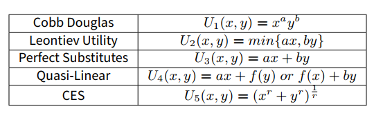
If we include uncertainty, we have (expected) utility functions. With risk aversion, we have others, such as constant relative risk aversion57 utilities, among others. If we include intertemporal choice, the rule family grows to include hyperbolically discounted utilities and its many relatives. With this variety in mind, then, let us pose the same question to economics.
Would the substitution of Leontiev’s utility \(U_{2}\) for Cobb-Douglas utility \(U_{1}\) be a small change in rules or a large one? Are quasi-linear utilities \(U_{4}\) with \(f(y) = ln(y)\) closer to perfect substitutes \(U_{3}\) than to CES (Constant Elasticity of Substitution) \(U_{5}\)? What could one mean by the distance between utility functions proper?58
For the space of real functions continuous on a compact domain, for example, an infinitude of metrics presents itself. Though I have not searched exhaustively, I have not encountered an article in Economics that argues for any one of them, or any Economics textbook recognizing this as an issue.59
So, “a small change in rules” (i.e., in the algebraic form of the utility function) is no clearer in Economics than in Agent-Based Modeling, or even Computer Science, where the distance between programs (equivalently, between partial recursive functions) is of no value or particular interest.
‘Agent models are not robust’
Detractors seem troubled that agent modeling is not robust to small changes in rules. But establishing such robustness would require us to usefully metrize rule space, which is challenging. However, it is no less challenging for Economics, where it is not even recognized as a problem, much less a fatal one.
In sum, while the search for useful metrics is a worthy problem, an inability to do this at present for ABMs is no more problematic than the same limit in Economics, or Logic, or Computer Science.
To complete the parallel, if the space of utility functions (as algebraic forms) cannot be metrized, can it be ordered? Of course it can, also in innumerable ways. But, would it be useful to say that the utility functions above (as algebraic forms) can be ordered (\(<\)) as \(U_{3} < U_{5} < U_{1} < U_{4} < U_{2}?\)60 This seems no less absurd than “Call home” preceding “Eat a pie” in a rule ordering.
‘Agent Models are Ad Hoc’
Closely related, ABMs are sometimes indicted as being Ad Hoc, by contrast to Economics with its allegedly unified theory of utility maximization. But, the theory hardly seems unified if one can choose from a virtually boundless menagerie of utility functions.61
Moreover, even the hypothesis that humans are maximizing any utility function is questionable, which brings us back to the rational actor. Some prominent defenders of this theory claim that critics are simply “poorly schooled.” Gintis (2018) writes, “Every argument that I have seen for rejecting the rational actor model I have found to be specious, often disingenuous and reflecting badly on the training of its author.”
Kenneth Arrow’s62 “training” can hardly be in doubt. Yet, as a cognitively plausible alternative to the rational actor, he offers a simple habit-driven (and irreversible) agent:
For example, habit formation can be made into a theory; for a given price-income change, choose the bundle that satisfies the budget constraint and that requires the least change (in some suitably defined sense) from the previous consumption bundle. Though there is an optimization in this theory, it is different from utility maximization; for example, if prices and income return to their initial levels after several alterations, the final bundle purchased will not be the same as the initial. This theory would strike many lay observers as plausible, yet it is not rational as economists have used that term. Without belabouring the point, I simply observe that this theory is not only a logically complete explanation of behaviour but one that is more powerful than standard theory and at least as capable of being tested.63
Rational Choice: Unfalsifiable or already falsified?
Countless articles in Economics take as their target an observed pattern (of consumption choice for example) and consider it to be explained when the pattern is shown to optimize a utility function meeting several mathematical requirements. Let us say that such utility functions are proper. Cleary, if for every possible choice \(x^{*}\) there is a theoretically proper64 utility function \(U\) such that \(x^{*}\) maximizes \(U\), then the general postulate of utility maximization is not falsifiable, as argued by Winter (1964) as well as others noted in Hodgson (2013). Relatedly, see Ledyard (1986).
That orthodox Rational Choice theory is either unfalsifiable or already falsified is a strong claim. However, it is fair to say that the settings in which it applies convincingly are less than universal, and that the theory is less unified than some would have us believe.
Part V: Agent_Zero and the Rational Actor
Therefore, a pressing aim of generative, and inverse generative, social science is to produce formal alternatives to the Rational Actor. Albeit simple and provisional, Agent_Zero (Epstein 2013) is one, in two central respects not elaborated before.65
First, Agent_Zero is directed at questions to which contemporary Rational Choice Theory (RCT) simply does not apply. Specifically, RCT does not concern the formation of political, economic, or other preferences. Adopting Stigler’s dictum, de gustibus non est disputandum,66 contemporary rational choice theorists militantly deny that the theory has anything to say about how people acquire baseless fears, genocidal hatreds, manifestly erroneous beliefs, logically inconsistent patterns of thought, self-injurious consumption preferences or any such thing. For a clear and unabashed statement, see Gintis (2018). As he insists, “The rational choice model expresses but does not explain individual preferences.”
The Rational Actor maximizes utility given whatever preferences (even if reprehensible or self-injurious) these internal fears and hatreds induce. In this modern orthodox usage of the term, if with sufficient strength an agent prefers more Aryan purity to less, it could be perfectly rational for him to join the Einsatzgruppen.67 If we care about how—by what cognitive or social processes—baseless fears and murderous dispositions come about, the Rational Choice theorist tells us to look elsewhere.
Some social scientists are interested in explaining how it is that genocidal utility functions happen—through combinations of unconscious emotions or “animal spirits” like fear, systematic errors in conscious appraisals of risks, amplified in social networks of other emotionally driven, poorly informed, and statistically hobbled peers. Rational choice theorists will aver that this question simply lies outside the ambit of RCT. Understood, but we are interested this, and moves like Agent_Zero are designed to study it.
That model posits specific, and I would say falsifiable, affective, deliberative, and social modules (mathematical expressions) grounded in cognitive neuroscience and psychology. These choices then are not ad hoc. In a provisional and fairly parsimonious68 way, Agent_Zero is directed at cognitive questions—how fears and attendant preferences arise, change, and spread—that are explicitly disavowed by rational choice theorists. This is one sense in which it is an alternative.
A core violation
However, Agent_Zero also concerns areas that are within the avowed scope of RCT, but violates a central canon of it. Specifically, in choosing a level of activity (production, consumption) rational actors set marginal benefit (MB) equal to marginal cost (MC).69 Agent_Zero does not, and knows he does not. There are two cases to consider: when Agent_Zero is attacked and when Agent_Zero is not attacked. Here, a compact demonstration is necessary.70
Case 1: Agent_Zero is attacked
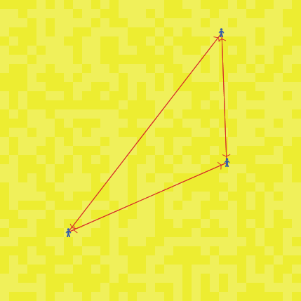
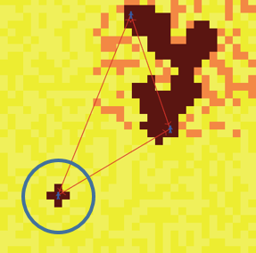
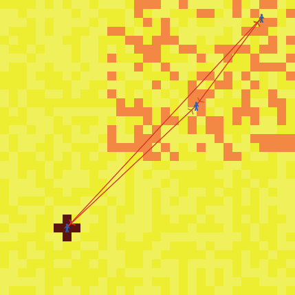
Figure 8 shows three connected (by red links) Agent Zeros (colored blue) occupying a landscape of indigenous agents, each of whom is simply a yellow patch, not a full Agent_Zero (yellow shades distinguish individuals).
Some indigenous agents in the northeast quadrant actively resist the occupiers, ambushing them at a random attack rate per “day.” When they do, their patch turns orange, “exploding,” as in Figure 9.
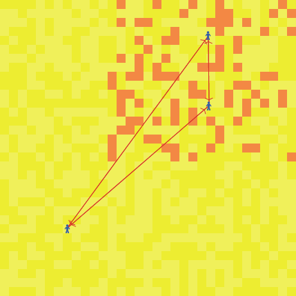
The two Agent_Zero occupiers in the volatile northeast are mobile (executing a 2D local random walk in their Von Neumann neighborhoods (the adjacent sites immediately to the north, south, east, and west of their location). The third Agent_Zero is stationary in the always-peaceful southwest. In this run, Agent “vision” (local sampling radius) is also limited to the Von Neumann neighborhood (and so is a sample selection bias).
The two attacked agents in the northeast unconsciously fear-condition (as in the Rescorla-Wagner model) on direct attacks, forming an association between yellow sites and the orange attacks. This is their affective, fear, component. They also consciously take in data and compute the moving average (over a memory length) of relative frequencies of attackers within their vision. This is their deliberative (empirical estimate) component. The sum of these is their solo disposition to retaliate. An agent’s total disposition is this solo disposition plus the sum of the weighted solo dispositions of the other Agent_Zeros in her (endogenous) network (fully-connected in this example). Solo disposition governs what Agent_Zero would do alone, while total disposition governs what it does in the group.
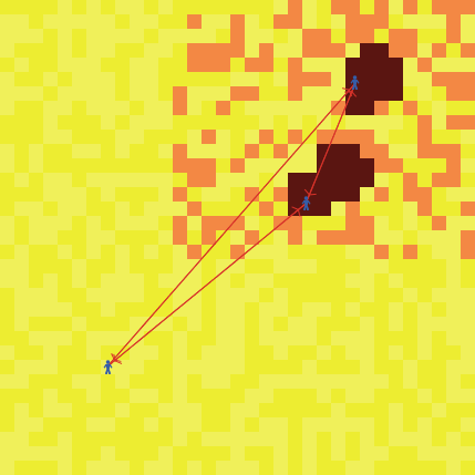
The agent’s behavioral repertoire is binary: destroy sites or not. She takes binary action—destroying all agents within a fixed destructive radius—if total disposition (\(D\)) exceeds an action threshold (\(\tau\)) or, more compactly, if total disposition net of the threshold (\(D_{net} \equiv D - \tau\)) is positive71 . Destroyed sites are colored dark (blood) red as shown in Figure 10.72
Their destruction reduces the aversive attack rate. Therefore, as noted earlier (Epstein & Chelen 2016) one could interpret Agent_Zero as a “disposition minimizer.”73 He doesn’t “like” having positive net disposition, or excess disposition to be economistic, and takes (binary) action to reduce it. Here, he destroys indigenous sites (whether attackers or innocents) within his destructive radius. This destructive action immediately reduces the rate of attacks and with it his destructive disposition.74 However, because fear may decay far more slowly, the killing can continue long after any evidentiary basis for it has vanished, as illustrated in Figure 11.
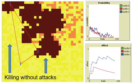
Here, the two mobile agents continue destroying benign sites lying outside the NE region of actual attacks. This destruction does not reduce the aversive attack rate. The incremental (marginal) benefit is therefore zero. If the incremental cost of retaliation is any positive number, then this behavior is economically irrational, in that marginal cost exceeds marginal benefit (which is zero). Now, the Rational Choice theorist might say, “Well, OK, but the agent perceives positive benefit.”
No! This is precisely the point: His deliberative module knows the benefit to be zero: It is returning an ambush probability of zero, as shown in the upper plot of Figure 11. But fear decays much more slowly, as shown in the lower plot. The killing persists after any empirical support for it has evaporated.75
Zillmann’s classic experiment
This is consistent with the behavior reported by Zillmann et al. (1975) in “Irrelevance of Mitigating Circumstances in Retaliatory Behavior at High Levels of Excitation.” They found that “Under conditions of moderate arousal, mitigating circumstances were found to reduce retaliation. In contrast, these circumstances failed to exert any appreciable effect on retaliation under conditions of extreme arousal.” That is, “the cognitively mediated inhibition of retaliatory behavior is impaired at high levels of sympathetic arousal and anger” (emphases added).
Purposive but not rational
Like the rational actor, Agent_Zero is clearly purposive. Unlike the rational actor, he is driven to engage in action he knows to be without benefit, continuing to kill even after his own calculation of the attack probability \(P(t)\) is zero. He does not reduce to homo economicus, who would choose a retaliation level that sets marginal benefit (incremental ambush relief) equal to marginal cost (of incremental retaliation). He continues acting until—through fear decay, attack cessation, and network effects—his total disposition is below threshold. In this respect, Agent_Zero might be considered a sticky “satisficer” (to invoke Simon 1956). Agent_Zero does not seek economic equilibrium.76 He seeks emotional equilibrium and emotions my change much more slowly than the facts.
Agent_Zero and the dual process literature
Beyond rational choice theory, this is also a departure from much of the “dual process” literature. The idea that humans have different—even competing–cognitive modes is not new to psychology. Tooby & Cosmides (2008) call them the “hot” and “cold” spheres of cognition. Schneider & Chein (2003) use the terms “automatic” and controlled." Stanovich & West (2000) introduced the terminology of System 1 and System 2, so adroitly deployed by Kahneman (2011) in his best-selling book, Thinking Fast and Slow.
These conceptual models have in common the important idea of a fast, automatic, effortless, and not necessarily conscious system (fear acquisition being exemplary) and a slow, conscious, and effortful system, as in statistical calculations. Kahneman is commendably clear that these Systems are “conceptual,” not mathematical. Like many useful idealizations, they are, he explains, convenient expository “fictions.” This literature provides many very important insights. It does not provide equations.
Since Agent_Zero’s Affective (fear) and Deliberative (relative frequentist) modules are mathematical, no strict correspondence, or isomorphism, between Kahneman’s or others’ two systems and Agent_Zero’s two internal (affective and deliberative) modules can be drawn, nor is one attempted. However, in certain settings, the analogy is inviting and — up to a point — the two stories “rhyme.”
For example, as discussed earlier, in the classic case of a snake thrown in one’s lap, fear acquisition (by LeDoux’s “quick and dirty” amygdaloid low road) is certainly faster than the conscious dispassionate appraisal of the threat (by LeDoux’s “slow but accurate” cortical high road). In this case, in acquiring fears—on the way up, so to say—System 1 (automatic) is typically faster than System 2 (deliberative).
However, on the way down, in expunging fears, the reverse may obtain. Where fear is high, the facts on the ground, and our conscious appraisal of them, can change much more rapidly than our emotions, as was illustrated by the plots in Figure 11. There, System 1, if I may, is the slow poke,77 a possibility Kahneman recognizes.
In connection with suicide bus bombings in Israel (analogous to our ambushes of Agent_Zero) he writes: “The emotional arousal is associative, automatic, and uncontrolled,” as in Agent_Zero’s Rescorla-Wagner associative fear-learning module. And, he continues," It produces an impulse for protective action," in Agent_Zero’s case, the disposition to retaliate. As in Figure 11 above, Kahneman writes, “System 2 may know that the probability is low, but this knowledge does not eliminate the self-generated discomfort and the wish to avoid it. System 1 cannot be turned off.” (emphasis added). But, if it cannot be turned off, then perforce System 1 is slower (since infinitely slow) to adapt to the changing facts than is System 2. Clearly, our Agent_Zero run “tells” the same general story mathematically. However, the story challenges any uniform ‘System 1 fast, System 2 slow’ picture, at least in this post-stimulus extinction phase.
Modules are sticky in their own ways
In this phase, Agent_Zero’s effortful deliberative module can also be “sticky.” It computes the moving average of local relative attack frequencies over a memory window. Thus, even if all fear-inducing attacks suddenly stop, it takes time to clear this memory or overwrite it with new experiences.78 Here the new experiences are zeros (no attacks). Thus, in “recovering from” its dispositions to act (e.g., to fight or to flee), Agent_Zero’s modules can each be ‘sticky in their own way.’
In Agent_Zero this is also possible the fear acquisition phase. Unlike the snake example—where the excitation level is high and fear is faster than deliberation–if the stimulus is neither surprising nor salient (producing a small fear learning rate), we may make a probability estimate before (or even without) any emotional response.
In Agent_Zero at least, and perhaps in humans, the general ‘fast vs slow’ relationship (in both the upward acquisition and downward extinction phases) is not uniform, and it may depend on excitation levels.
Rates and levels
Clearly, some (e.g., Zillmann) are focused on excitation levels. Which module has greater magnitude, the emotional module or the mitigating deliberative one? Others (e.g., Kahnemann) are focused on excitation rates, or which module (or System) is faster. But what really matters in terms of action? Is it which module is faster, or which is bigger, and is there any uniform relationship between them?
Again, without purporting to mathematize Zillmann’s or Kahneman’s picture, in Agent_Zero, one module could be faster but smaller than the other, or slower but bigger, and so forth. Moreover, the “speed-lead” could change hands with one module remaining bigger (i.e., dominant) throughout, and vice versa, all of which is under unified mathematical study.79
Purposive but not rational
Returning to our specific scenario, like the rational actor, Agent_Zero is clearly purposive. Unlike the rational actor, he engages in action he knows to be without benefit, continuing to kill even after \(P(t) = 0\). In this setting, he does not reduce to a utility maximizer, choosing a retaliation level that sets a marginal benefit (incremental ambush relief) equal to a marginal cost (of incremental retaliation). He continues acting until—through fear decay, attack cessation, and network effects—his total disposition is below threshold.
All of the above holds for the mobile agents in Figure 9, who at least initially are subject to attacks.
Case 2: Agent_Zero not attacked
The deeper and more disturbing case is the southern Agent_Zero who is never attacked, but who acquires excess retaliatory disposition purely through the disposition of remote others. The southwest Agent_Zero wipes out his village although (unlike the northeast agents) no villager has attacked him, a parable80 of the My Lai massacre. For this agent, there never were any attacks, so there is no aversive stimulus to reduce through destructive retaliation. Throughout, destruction occurs without benefit. Again, since the marginal benefit of violence is zero,81 if violence carried any incremental cost,82 no classically rational agent would engage in it83 (because marginal cost would again exceed marginal benefit). Agent_Zero does engage in it, despite knowing (by the deliberative module) the objective attack probability to be zero within his vision (the blue circle), as shown in Figure 12.
He joins the lynch mob, as it were, having had no adverse experience with black people. He does things in the group that he would not do alone. In the extreme case, he is the first to do them. He leads the lynch mob! This is shown in Figure 13.
The two attacked agents in the northeast have positive but sub-threshold retaliatory dispositions. Each is “distressed,” but not enough to retaliate. However, the sum of their weighted dispositions drives the never-attacked southern agent over his threshold,84 and he wipes out the innocent village. Again, his deliberative module has told him they are innocents.85 Moreover, the agent can continue acting (e.g., killing) while his deliberative module is reporting no probability of attack.
Hume revisited
Regarding ‘dual process’ Hume, then, reason is not only “a slave to the passions,” but knows itself to be! Of course, this is all too human. We continue eating knowing the marginal benefit of further cookies to be zero (indeed negative!). People with post-traumatic stress continue to fear events they know to have probabilities near zero.86
This southern agent’s initiation of violence occurs by a cognitive mechanism of dispositional contagion, not rational choice or imitation. The latter is obviously not possible for the first actor, since there is no one yet to imitate, as is clear in Figure 13. In joining or initiating an action he would not take alone, one might say that Agent_Zero betrays himself. In the most extreme case–the book’s Jury Trial–all agents do. Alone, each would acquit. Together in the jury chamber, they unanimously convict!87 It is universal self-betrayal.
These behaviors simply fall outside the ambit of the rational actor, but unfortunately fall well within that of the human being, all of which led me to write:
"The overall picture of Homo sapiens reflected in these interpretations of Agent_Zero is unsettling: Here we have a creature evolved (that is, selected) for high susceptibility to unconscious fear conditioning. Fear (conscious or otherwise) can be acquired rapidly through direct exposure or through observation of fearful others. This primal emotion is moderated by a more recently evolved deliberative module which, at best, operates suboptimally on incomplete data, and whose risk appraisals are normally biased further by affect itself. Both affective and cognitive modules, moreover, are powerfully influenced by the dispositions of other—equally limited and unconsciously driven—agents. Is it any wonder that collectivities of interacting agents of this type—the Agent_Zero type—can exhibit mass violence, dysfunctional health behaviors, and financial panic?" (Epstein 2013 p.188)
If we are interested in the cognitive wellsprings of such collective phenomena, models like Agent_Zero may be a more fertile starting point (a better “ideal gas”) than the rational actor. But, the Agent_Zero I designed (intelligently, I would hope) is not the last word, as emphasized earlier.
A modest proposal: Grow Agent_Zero
Specifically, it would be very interesting to “disassemble” Agent_Zero into its primitive rule constituents (Darwin’s warm little pond) and extend that set with alternative primitives. Several of these are offered in the published Agent_Zero code,88 and others have been proposed elsewhere.89 One would also allow combinators beyond those thus far employed, allowing nonlinear entanglement between modules, and use iGSS to discover other, perhaps fitter, agents in this algorithmic phylum and others. It is conceivable that in some settings, the original Agent_Zero is re-evolved as the winner. But, it might also be fundamentally modified with some elements conserved (as in the Gunaratne et al. 2023 Schelling model above), or it might be skipped altogether! It would be progress either way.
Part VI. Concluding Thoughts
We have reviewed the epistemology of generative social science, have discussed iGSS as a means to discover generative agent architectures and rules, and have introduced examples presented fully in the articles that follow in this Special Section. They (and many others not included here) exhibit several distinctive advantages of the approach:
First, iGSS can evolve novel generative agents that might have eluded even very intelligent human designers.
Second, it can produce a set of them — multiple generators — subsets of which may be comparably fit (well-calibrated to the target). The adjudication or ranking of these multiple competitors may require new micro-data, or experiments at the micro scale.
Third, some of these sets of comparably fit agents exhibit elements that are conserved across algorithmic evolution, just as the amygdala has been conserved across vertebrate evolution. While we cannot rigorously define neighborhoods of agents (which requires that we metrize rule space), we might define families (or phyla) of agents by these conserved elements.
Fourth, there is no general relationship between rule fitness and rule complexity. In some cases (Vu et al. 2023) there is a steep tradeoff. By contrast, in Gunaratne et al. (2023), the fittest evolved rule is among the simplest, and vastly simpler than the runner up. Moreover, the relationship between rule fitness and complexity is not even monotone.90 There has been a widespread presumption that Genetic Programing must produce highly complex and opaque expressions. Here is a counter-example.
Fifth, several of the articles in the present collection enforce that algorithmic evolution (as in many Genetic Programs) can exhibit jumps, or punctuated equilibria, which are also observed in biological evolution.
Unlike biological evolution, however, all of this can start (without fear of infinite regress) with an intelligently designed base model, which can be deconstructed into primitive constituents to be mutated, crossed, and concatenated to yield new explanatory alternatives. I offer Agent_Zero as one such Garden-of-Eden candidate, though there are doubtless many others.
Far from being “The End of Theory,” iGSS offers a resurgence of it. The locus of theoretical work shifts from the completed agent architecture to its constituents and their permissible combinations. This can be every bit as creative as the traditional design of entire agents, which we would certainly expect to continue.
Some of these agent constituents (like a fear learning rule module) are not conscious at all, much less rational. The scope of this programme is broader than Rational Choice Theory, which disavows any attempt to explicate cognitive drivers of social preference or bias, where Agent_Zero includes them explicitly and falsifiably. In areas of interest to both theories, moreover, Agent_Zero is not canonically rational. He acts knowing the benefit (e.g., reduction in the attack rate) to be zero. The assumption that action carries any cost whatsoever makes his continued killing irrational: \(\text{MC > MB}\).
The agent does not seek economic equilibrium, but emotional equilibrium, as it were. And emotions may change much more slowly than the facts. Moreover, in many setting they should! It would make no evolutionary sense to learn to fear alligators on Monday and then forget to on Tuesday. Hard-wired fear retention91 provides long-term selective advantage, but as we see, it can override short-term economic optimization. Evolution can trump economics.
This contrasts with RCT but also with some of the qualitative dual process (hot/cold, fast/slow) literature as well. In Agent_Zero, the speeds and the magnitudes of the Affective and Deliberative Modules—in both acquisition and extinction phases—depend on the context (e.g., the threat dynamic) and specific initial agent conditions and parameters, plus endogenous social network dynamics. The same is true for the nonviolent interpretations of Agent_Zero, such as physical flight from disasters or contagious fear-driven flights from financial portfolios (Epstein 2013). The complete mathematics of this, initially for Agent_Zero, is a fruitful line of theoretical and possibly experimental work.
For several fundamental anomalies of Rational Choice Theory (e.g., endowment effects and asymmetrical weights on gains and losses), Prospect Theory (Kahneman & Tversky 1979) offers an elegant formal solution. For the different cognitive drivers and economic anomalies (as where MC > MB) of interest to Agent_Zero, a different, and generative, formalism is required.92 With Agent_Zero, I hope to have provided a starting point and, in iGSS, an evolutionary way forward.
The need for suitable data
Data (“big” or small) are not theory and cannot replace theory. Without suitable data, however, there is no empirical selection pressure on competing theories. And, without such pressure, no science, including iGSS itself, can progress. That said (staying with biological analogies), “off-the-shelf” public data sets often strike me as the “fossil record” of past funding decisions by government agencies and foundations. Like the true fossil record, there are many gaps. If we have a specific new theory, but the available data were collected without that specific theoretical motivation, it is not surprising that the data, however “big,” may not be suited to test that theory.
As often happens in science, new theory may precede and require the collection of new data. Without Maxwell’s theory, no one would have known to look for radio waves, whose existence he deduced mathematically. Without relativity theory, no one would have thought to measure the predicted deflection of light in a gravitational field. Science does not always begin with data. It sometimes begins with a theory, which tells us what data to collect.
Perhaps this is the case with (the incomparably more modest) Agent_Zero. Luckily, there are many exciting new data sources—from cognitive neuroscience to innovative laboratory experiments to natural experiments unfolding on social media—that can and should be brought to bear in testing and attempting to falsify it. “Off-the-shelf” data sets (and existing statistical methods93) may be not be well-suited to either its corroboration or refutation, though I am happy to be corrected.
Backward to the future
Popper (1962) characterized scientific progress as a process of Conjectures and Refutations. Our allegiance must be to this process, not to any particular conjecture, the Rational Actor and Agent_Zero included. Inverse (or backward) Generative Social Science can evolve a much larger space of competing generative candidates—each a conjecture—than we can yet design by hand. Fisher's (1930) Fundamental Theorem of Natural Selection is that the rate of growth in average fitness is proportional to phenotypic variance. By driving up the variance in generative agent phenotypes, iGSS can likewise accelerate the evolution of social science.
Acknowledgements
For detailed reading, editorial suggestions, and countless invaluable discussions, I thank Erez Hatna. For penetrating reviews with many editorial suggestions, I thank Duncan Foley, Scott Page, and Paul Slovic. For many useful comments and clarifications, I thank Jeewoen Shin, my JASSS co-authors, and other colleagues in the present collection. For important consultations, I thank Melissa Healy. For his suggestions on the manuscript, his early and sustained support for iGSS, and for encouraging this Special Section, I thank Flaminio Squazzoni. I also thank the paper’s two anonymous reviewers, whose many insights led me to clarify and restructure the manuscript. All opinions expressed are those of the author alone. This research was supported by the National Institutes of Health under project CASCADE, R01 AA024443.
Appendix A
The original version of the document "Using GAs to Grow Artificial Societies (1992)" is included.
Appendix B
The original version of the document "Artificial Social Life (1992)" is included.
Notes
This essay is based on addresses at the first two International Workshops (2020 and 2021) on iGSS, held in the US, and at the 2022 SCC and iGSS Panel held in Milan, Italy as well as invited Talks at The University of Chicago, The Fields Institute for Research in Mathematical Sciences, Toronto; The Turing Institute, London; Alphabet, Mountain View CA; Tsinghua University, Beijing; the OECD, Paris, and the Courant Institute of Mathematical Sciences at NYU.↩︎
The present collection is focused on Evolutionary Computation. Other AI methods including Machine Learning are also applicable.↩︎
Though distinct from this specific agenda, related lines of work include inductive game theory (DeDeo et al. 2010), rule induction (Rand 2019), computational abduction (Ren et al. 2018), and the evolution of optimal strategies in the repeated prisoners dilemma (Axelrod 1987; Lindgren & Nordahl 1994).↩︎
For a recent literature review see (co-published in English and Russian) Makarov et al. (2022).↩︎
For difficulties in Kuhn’s use of this and related terms, see Joseph Epstein (1979). I have in mind simply a set of common practices, here the conscious design of complete agents to generate targets, as distinct from their computational evolution from primitive agent constituents.↩︎
For subsequent articulations, see Epstein (1999, 2006, 2019)↩︎
Hence my subtitle↩︎
“When” is technically unnecessary, since we can subsume it in “that” by saying that it will rain today at noon.↩︎
See also Troitzsch (2009), from which I stand corrected on epicycles.↩︎
One might argue that autonomy was another.↩︎
Technically, it depends on the numerical values returned by the affective and deliberative modules, each of which is a real-valued function defined on the stochastic stimulus landscape, and bounded to [0,1].↩︎
For a mathematical discussion of how the affective, deliberative, and social modules could be rendered as orthogonal basis elements for a space of cognitively plausible agents, see Epstein (2013) (fn. 24).↩︎
Named after John Nash, Nobel Laureate in Economics↩︎
As in coordination game “poverty traps.”↩︎
The well-known reasoning is that on the final 100th one-shot game, each should certainly defect, because retaliation is not possible. But since the optimal behavior on the 100th game is determined, the players should defect in the (now effectively final) 99th, and so forth back to the first game.↩︎
On the multiplicity of Bayesian-Nash equilibria, see Ledyard (1986).↩︎
Gary Becker, Nobel Laureate in Economics.↩︎
By “positive,” I believe Keynes means simply “definite” or “concrete,” not meritorious.↩︎
In some classes of infinite games, the optimization problem is literally unsolvable in pure strategies (Prasad 1991).↩︎
For a penetrating philosophical critique, see Nagel (1963).↩︎
For a critique of selectionist arguments for the maximization hypothesis, see Winter (1964) and others discussed in Hodgson (2013).↩︎
For example, the assumption that all agents are conforming, optimizing in the Bellman sense, is not consistent with the macro data on the timing of retirement. See Axtell & Epstein (1999).↩︎
In fact, Becker and Murphy’s paper does not mention the neurobiology of addiction, or offer a single reference to the scientific literature on it.↩︎
Analogously in mathematics, not everything can be a nontrivial Theorem. There must be Axioms (trivially theorems since A implies A) that are not themselves deduced from antecedent propositions.↩︎
Just for completeness sake, neither are we insisting that Physics adopt our generative explanatory standard. We are talking about social science broadly construed where we are insisting that explananda (be they meso- or macro-scale) be generated in populations of cognitively plausible individuals. Whatever may be one’s definition of cognitive plausibility, electrons surely fail.↩︎
G \(\supset\) E is the converse of \(\neg\) G \(\supset\) \(\neg\) E because by contraposition, the latter is E \(\supset\) G.↩︎
One impressive example is the alternative plot-selection rules for the ancient Anasazi, evolved by Gunaratne & Garibay (2020). These evolved rules outperform our original rules (Axtell et al. 2002), at the cost of somewhat more (but hardly intolerable) rule-complexity. Accuracy (i.e., fitness) versus complexity is a central topic discussed below.↩︎
Each of these is an explicit bounded real-valued mathematical function. Both differential equation and agent-based computational versions are given in Epstein (2013).↩︎
Arguments that affective homophily is a sensible starting point are given in Epstein (2013). The published Agent_Zero code allows one to select two alternatives.↩︎
One among many is temporal-difference learning (Sutton & Barto 1987).↩︎
The published code allows the user to choose a moving median for example.↩︎
The memory length is user-specified.↩︎
The published code allows the user to choose probability homophily and disposition homophily, for example.↩︎
One way (Epstein 2013) to have fear bias the agent’s probability estimate is to set \(p_{e} = p^{1 - V}_{n}\), where \(P_{e}\) is the emotionally biased estimate, \(P_{n}\) is the emotionally neutral estimate, and \(V \in [0, 1]\) is the fear level. With no fear (\(V = 0\)), there is no bias. But if petrified by shark attack (\(V = 1\)), we don’t go near the water, imagining an attack as all but certain.↩︎
Of course, the documented anomalies are myriad, including framing and endowment effects, asymmetric weights on gains and losses, reliance on heuristics, base rate neglect, anchoring, preference reversals, and the Ellsberg and Allias paradoxes, to name several.↩︎
One such is disgust, routinely mobilized in propaganda to induce (by conditioning) a nefarious association between the enemy and an irksome insect, rodent, or festering disease. We do not choose to be disgusted by a hideous smell or taste. We simply recoil in revulsion. As Chapman & Anderson (2012) write, “The anterior insula, and to a lesser extent the basal ganglia, are implicated in toxicity- and disease-related forms of disgust, although we argue that insular activation is not exclusive to disgust.”↩︎
If we define “sound” as an auditory sensation occurring only when these waves collide with a human eardrum, then the ancient puzzle is resolved: “No, isolated from human eardrums, the falling tree produces no sound, though it does disturb the medium.” And vice versa if “sound” is defined simply as the disturbance.↩︎
That a machine or monkeys at typewriters might eventually produce Hamlet—the same output as William Shakespeare—does not illuminate how Shakespeare wrote plays.↩︎
On ChatGPT specifically, see Chomsky (2023).↩︎
For instance, see “More data usually beats better algorithms,” at Datawocky: https://anand.typepad.com/datawocky/2008/03/more-data-usual.html.↩︎
More generally an \(\epsilon\)-machine (Shalizi & Crutchfield 2001).↩︎
The norm of a difference between functions is a metric. In general, for a real number \(p \geq 1\), the \(p-\)norm of \(x\) is defined as: \(\left\|x_{p}\right\| = (\lvert x_{1} \rvert^{p} + \lvert x_{2} \rvert^{p} \dots + \lvert x_{n} \rvert^{p})^{\frac{1}{p}}\). MSE is based on the \(L_{2}\) norm.↩︎
I would not assume that cognitively plausible internal agent rules will necessarily be easy for an external human to interpret. There are cognitively plausible, indeed empirically supported, internal rules whose functional form is very hard to interpret, as in neural network learning dynamics.↩︎
There might be multiple peaks of equal height or none, as on unbounded sets.↩︎
Also known as “Darwin’s bump”, this is a small cartilaginous nub on the inside of the upper ear, with no apparent function (Darwin 1871)↩︎
English is but one example.↩︎
I first heard this idea from Ivan Garibay.↩︎
These additions produce stepwise advances, or punctuated equilibria, as we discuss below.↩︎
This, of course, is an entirely separate question from whether any of these auto-calibrated models works well in novel, out-of-sample settings, sometimes called “external validation.”↩︎
Admittedly, economic factors would likely play a role in one’s pattern, or habit, of movement since multiple moves cumulates costs.↩︎
I have not encountered a model in microeconomics where different agents have utility functions of different algebraic forms.↩︎
Heterogeneous agent macroeconomics is in fact a vibrant area. See Hommes & LeBaron (2018).↩︎
While it makes the point, this is a slight abuse since, technically, the number of permutations is not necessarily the same as the Hamming Distance.↩︎
Not to be confused with the += operator in C++↩︎
We also cannot construct an analogue of Structural Stability for agent-models. This would require that the notion of a neighborhood of rules—all those within distance \(d\) of one another—be formalized and in addition that an analogue of homeomorphism (not distance) between outputs (phase portraits) be devised. No obvious approach presents itself.↩︎
Problematic for the rightmost rule.↩︎
These subsume logarithmic utilities.↩︎
Notice that to say, “Well, from the economic context, we will know which \(U\) is most suitable” is irrelevant to the question at hand: whether the space of Us can be usefully metrized, so that robustness to “small changes” in form could be assessed.↩︎
Although their definition of “departure from rationality” does not involve these metric considerations, Akerlof & Yellen (1985) take a very interesting step in this direction in their AER article “Can Small Deviations from Rationality Make Significant Differences to Economic Equilibria?” Their answer is yes.↩︎
Lexicographic preferences raise the problem of just noticeable differences in microeconomics.↩︎
Of course, the range of candidates may be constrained by the economic setting, but few settings would preclude all but one functional form.↩︎
Nobel Laureate in Economics.↩︎
- Arrow (1990)↩︎
See Gintis (2018) or a graduate microeconomics text, such a Kreps (2020).↩︎
Several anomalies, such as endowment effects and loss aversion are, of course, addressed formally by Prospect Theory (Kahneman & Tversky 1979). Agent_Zero addresses other concerns.↩︎
‘We do not argue about tastes.’↩︎
For a colorful rendition of the general point, see Kahneman (2011 p. 411).↩︎
Landscape settings aside, Agent_Zero proper contains six parameters: the affective learning rate, the moving average memory, the action threshold (all equal in the book), the maximum associative strength (equal and set to the usual default of 1 in the book), and the vision and destructive radii (all equal in the book). Network weights are endogenous so do not add parameters. The code offers two nonlinear extension parameters for the affective module, which are not employed in the basic published Agent-Based computational runs. See the source code in Epstein (2013 Appendix III) or under the code tab at http://modelingcommons.org/browse/one_model/5982#model_tabs_browse_nlw↩︎
Thinking of firms, at each level of production, \(q\), the firm’s economic profit \(\pi (q)\) is by definition its revenue \(R(q)\) minus its production cost \(C(q)\). That is, \(\pi (q) = R(q) - C(q)\). At a profit maximum, \(\pi ^{'} (q) = 0\). But because the derivative is a linear operator, we have \(R^{’}(q) = C^{’}(q)\): marginal benefit (here revenue) MB equals marginal cost MC. It applies to myriad activities, including the optimal level of costly retaliation. A rational actor will cease when MB = MC. Agent_Zero (a) continues beyond this point (MC > MB) and (b) knows he is beyond this point.↩︎
All equations, code, and numerical assumptions are given in Epstein (2013).↩︎
If the agent is operating alone then the total disposition equals solo disposition.↩︎
An animated movie of this run is posted at https://vimeo.com/83069872. The NetLogo code can be run online at http://modelingcommons.org/browse/one_model/5982#model_tabs_browse_nlw.↩︎
In fact, I did not design Agent_Zero with this interpretation in mind and thank Erez Hatna for recognizing it. As stated in Epstein & Chelen (2016), “While Agent_Zero is not canonically rational, this agent is arguably purposive. One can think of Agent_Zero as taking actions that seek to reduce aversive stimulus: wiping out attacking sites, or fleeing contaminated ones. In acting to minimize aversive stimulus, Agent_Zero could be interpreted as a disposition minimizer.”↩︎
The complete technical mechanism is (i) the extinction of fear (in the affective module) (ii) the reduction in the relative frequency of attacks (in the deliberative module), and (iii) their contagion effects through the network. If the updated total disposition is below his retaliation threshold, he desists . Otherwise, he continues.↩︎
This is a “fight” scenario. Agent_Zero exhibits the same irrational behavior in the “flight” scenario in Epstein (2013). There, Agent_Zero continues fleeing (which carries some marginal cost) long after he knows he has escaped the contaminated zone (marginal benefit being exposure-reduction, which is zero outside the toxic zone).↩︎
Technically it is dispositional equilibrium.↩︎
For the innocent population, this is disastrous.↩︎
This is modeled in the 18th Brumaire of Agent_Zero (Epstein 2013 pp. 165–168).↩︎
To give the flavor of his work, recall that the modules are functions returning numbers. Then, if the modular levels at time \(\tau\) are \(V(\tau)\) and \(P(\tau)\), we define their speeds as the absolute values of their derivatives: \(\lvert V^{'}(\tau) \rvert\) and \(\lvert P^{'}(\tau) \rvert\), making the speed of change independent of its direction (up or down). In this notation, \(V\) is larger but slower if \(V(\tau) > P(\tau)\) and \(\lvert V^{'}(\tau) \rvert < \lvert P^{'}(\tau) \rvert\). In turn, \(P\) is larger and faster if \(V(\tau) < P(\tau)\) and \(\lvert V^{'}(\tau) \rvert < \lvert P^{'}(\tau) \rvert\), and so forth. Moreover, there may be times \(\tau^{*}\) at which the ‘speed-lead’ switches from one module to the other, but the ‘size-lead’ does not. This would be the case if on some time interval: (a) For \(\tau < \tau^{*}\) we have \(\lvert V^{'}(\tau) \rvert < \lvert P^{'}(\tau) \rvert\), (b) For \(\tau > \tau^{*}\) we have \(\lvert V^{'}(\tau) \rvert > \lvert P^{'}(\tau) \rvert\), but (c) For the entire interval, \(V(\tau) > P(\tau)\). All these possibilities, and their connection to total disposition and action can be studied concretely in Agent_Zero, where explicit formulas for \(V\) and \(P\) are given. This abstract rendition is continuous, but the discrete time analogue is of course constructible and characteristic of the agent-based version.↩︎
All runs are called Computational Parables.↩︎
Because the derivative of a constant (here zero) is zero.↩︎
Although it is easily done, we have not introduced any explicit cost-of-retaliation function here. The point stands if we simply agree that killing requires some non-zero expenditure of effort, time, or resources, which hardly seems debatable.↩︎
Nor, by the same logic, would the two northeastern Agent_Zeros continue their slaughter of innocents outside the ambush area, as they do later in this run with a zero fear-extinction rate. See Epstein (2013 Figure 38, p.92)↩︎
Action thresholds are equal here.↩︎
As a commentary on the human condition, this seems more significant than the technical point that any positive marginal cost exceeds the zero marginal benefit, which still applies.↩︎
Agent_Zero is afflicted with PTSD in Epstein (2013 pp. 78–79).↩︎
Compactly, for every agent, \(D_{total} > \tau > D_{solo}\)↩︎
Already coded alternatives are offered in Epstein (2013). As deliberative alternatives, I offer the choice of moving average or moving median. As affective alternatives, I offer classic Rescorla-Wagner and nonlinear variants. To form endogenous network weights, the user can select affective, probability, or dispositional homophily. And of course, the entire model can be scaled up indefinitely.↩︎
See Figure 6 of Gunaratne et al. (2023).↩︎
Implemented through long-range potentiation. See LeDoux (2002).↩︎
It could be very interesting to use the prospect-theoretic value function as a module of Agent_Zero.↩︎
For a “call to arms,” by two statisticians, on the need for new statistical methods to test ABMs generally, see Banks & Hooten (2021)↩︎
References
AKERLOF, G. A., & Shiller, R. J. (2010). Animal Spirits: How Human Psychology Drives the Economy, and Why It Matters for Global Capitalism. Princeton, NJ: Princeton University Press.
AKERLOF, G. A., & Yellen, J. L. (1985). Can small deviations from rationality make significant differences to economic equilibria? The American Economic Review, 75(4), 708–720.
ALLAIS, M. (1953). Le comportement de l’homme rationnel devant le risque, critique des postulats et axiomes de l’´ecole Americaine’. Econometrica, 21, 503–546.
ANDRIANAKIS, I., Vernon, I. R., McCreesh, N., McKinley, T. J., Oakley, J. E., Nsubuga, R. N., Goldstein, M., & White, R. G. (2015). Bayesian history matching of complex infectious disease models using emulation: A tutorial and a case study on HIV in Uganda. PLoS Computational Biology, 11(1), e1003968.
ARIELY, D. (2008). Predictably Irrational: The Hidden Forces That Shape Our Decisions. New York, NY: Perennial.
ARROW, K. J. (1990). Economic theory and the hypothesis of rationality. In J. Eatwell, M. Milgate & P. Newman (Eds.), Utility and Probability, (pp. 25–37). London: The New Palgrave Macmillan
AXELROD, R. (1987). The evolution of strategies in the iterated prisoner’s dilemma. The Dynamics of Norms, 1, 1–16.
AXTELL, R. L. (2016). 120 million agents self-organize into 6 million firms: A model of the US private sector. Proceedings of the 2016 International Conference on Autonomous Agents & Multiagent Systems.
AXTELL, R. L., & Epstein, J. M. (1999). Coordination in transient social networks: An agent-based computational model of the timing of retirement. In H. Aaron (Ed.), Behavioral Dimensions of Retirement Economics. Washington, DC: Brookings Institution Press and Russell Sage Foundation. [doi:10.2307/j.ctv36mk90z]
AXTELL, R. L., Epstein, J. M., Dean, J. S., Gumerman, G. J., Swedlund, A. C., Harburger, J., Chakravarty, S., Hammond, R., Parker, J., & Parker, M. (2002). Population growth and collapse in a multiagent model of the Kayenta Anasazi in Long House Valley. Proceedings of the National Academy of Sciences, 99(3), 7275–7279.
BANKS, D. L., & Hooten, M. B. (2021). Statistical challenges in agent-based modeling. The American Statistician, 75(3), 235–242. [doi:10.2307/1907921]
BECKER, G. S., & Murphy, K. M. (1988). A theory of rational addiction. Journal of Political Economy, 96(4), 675–700. [doi:10.1371/journal.pcbi.1003968]
BERWICK, R. C., Pietroski, P., Yankama, B., & Chomsky, N. (2011). Poverty of the stimulus revisited. Cognitive Science, 35(7), 1207–1242.
CAPRARO, V., Jordan, J. J., & Rand, D. G. (2014). Heuristics guide the implementation of social preferences in one-shot Prisoner’s Dilemma experiments. Scientific Reports, 4(1), 1–5. [doi:10.1007/978-1-349-20568-4_8]
CHAPMAN, H. A., & Anderson, A. K. (2012). Understanding disgust. Annals of the New York Academy of Sciences, 1251(1), 62–76.
CHOMSKY, N. (1965). Aspects of the Theory of Syntax. Cambridge, MA: MIT Press.
CHOMSKY, N. (2009). Turing on the “Imitation Game”. In R. Epstein, G. Roberts, & G. Beber (Eds.), Parsing the Turing Test (pp. 978–971). Dordrecht: Springer Netherlands.
CHOMSKY, N. (2023). The false promise of ChatGPT. The New York Times. March 8. Available at: https://www.nytimes.com/2023/03/08/opinion/noam-chomsky-chatgpt-ai.html. [doi:10.1073/pnas.092080799]
DARWIN, C. (1871). The Descent of Man and Selection in Relation to Sex. London: John Murray. [doi:10.1080/00031305.2021.1900914]
DAWES, R. M. (2001). Everyday Irrationality. Boulder, CO: Westview Press. [doi:10.1086/261558]
DEDEO, S., Krakauer, D. C., & Flack, J. C. (2010). Inductive game theory and the dynamics of animal conflict. PLoS Computational Biology, 6(5), e1000782. [doi:10.1111/j.1551-6709.2011.01189.x]
EDMONDS, B., Le Page, C., Bithell, M., Chattoe-Brown, E., Grimm, V., Meyer, R., Montañola-Sales, C., Ormerod, P., Root, H., & Squazzoni, S. (2019). Different modelling purposes. Journal of Artificial Societies and Social Simulation, 22(3), 6. [doi:10.1038/srep06790]
ELLSBERG, D. (1961). Risk ambiguity, and the savage axioms. Quarterly Journal of Economics, 75, 643–649. [doi:10.1111/j.1749-6632.2011.06369.x]
EPSTEIN, J. (1979). Review of Thomas S. Kuhn, the essential tension. American Journal of Physics, 47(6), 568–570. [doi:10.21236/AD0616323]
EPSTEIN, J. M. (1998). Zones of cooperation in demographic prisoner’s dilemma. Complexity, 4(2), 36–48.
EPSTEIN, J. M. (1999). Agent‐based computational models and generative social science. Complexity, 4(5), 41–60.
EPSTEIN, J. M. (2006). Remarks on the foundations of agent-based generative social science. Handbook of Computational Economics, 2, 1585–1604. [doi:10.5962/bhl.title.24784]
EPSTEIN, J. M. (2008). Why model? Journal of Artificial Societies and Social Simulation, 11(4), 12.
EPSTEIN, J. M. (2013). Agent_Zero. Princeton, NJ: Princeton University Press. [doi:10.1371/journal.pcbi.1000782]
EPSTEIN, J. M. (2019). Inverse generative social science: What machine learning can do for agent-based modeling. In P. Davis, A. O’Mahony, & J. Pfautz (Eds.), Social-Behavioral Modeling for Complex Systems. Hoboken, NJ: John Wiley & Sons. [doi:10.18564/jasss.3993]
EPSTEIN, J. M., & Axtell, R. (1996). Growing Artificial Societies: Social Science From the Bottom Up. Cambridge, MA: MIT Press. [doi:10.2307/1884324]
EPSTEIN, J. M., & Chelen, J. (2016). Advancing agent_zero. In D. S. Wilson & A. Kirman (Eds.), Complexity and Evolution: Toward a New Synthesis for Economics. Cambridge, MA: MIT Press. [doi:10.1119/1.11776]
EPSTEIN, S. D., & Hornstein, N. (Eds.). (1999). Working Minimalism. Cambridge, MA: MIT Press. [doi:10.1002/(SICI)1099-0526(199811/12)4:2<36::AID-CPLX9>3.0.CO;2-Z]
FISHER, R. A. (1930). The Genetical Theory of Natural Selection. Oxford: Clarendon Press. [doi:10.1002/(SICI)1099-0526(199905/06)4:5<41::AID-CPLX9>3.0.CO;2-F]
FLOOD, M. M. (1958). Some experimental games. Management Science, 5(1), 5–26. [doi:10.1016/S1574-0021(05)02034-4]
FRIEDMAN, M. (1953). The methodology of positive economics. In M. Friedman (Ed.), Essays in Positive Economics. Chicago, IL: University of Chicago Press.
GINTIS, H. (2018). Rational choice explained and defended. In G. Bronner & F. Di Iorio (Eds.), The Mystery of Rationality (pp. 95–114). Berlin Heidelberg: Springer.
GOULD, S. J., & Eldredge, N. (1972). Punctuated equilibria: An alternative to phyletic gradualism. Models in Paleobiology, 1972, 82–115.
GÖDEL, K. (1931). Ub̈er formal unentscheidbare Sätze der Principia Mathematica und verwandter Systeme I. Monatshefte Für Mathematik Und Physik, 38(1), 173–198. [doi:10.7551/mitpress/3374.001.0001]
GREIG, R., & Arranz, J. (2023). Learning interpretable logic for agent-Based models from domain independent primitives. Journal of Artificial Societies and Social Simulation, 26(2).
GUNARATNE, C., & Garibay, I. (2020). Evolutionary model discovery of causal factors behind the socio-agricultural behavior of the ancestral Pueblo. PLoS ONE, 15(12), e0239922. [doi:10.7551/mitpress/7305.001.0001]
GUNARATNE, C., Hatna, E., Epstein, J. M., & Garibay, I. (2023). Generating mixed patterns of residential segregation: An evolutionary approach. Journal of Artificial Societies and Social Simulation, 26(2), 7. [doi:10.5962/bhl.title.27468]
HAMILTON, A. G. (1988). Logic for Mathematicians. Cambridge: Cambridge University Press. [doi:10.1287/mnsc.5.1.5]
HODGSON, G. M. (2013). From Pleasure Machines to Moral Communities. An Evolutionary Economics Without Homo Economicus. Chicago, IL: University of Chicago Press.
HOMMES, C., & LeBaron, B. (2018). Introduction to the Handbook of Computational Economics, Volume 4, Heterogeneous Agent Modeling. In C. Hommes & B. LeBaron (Eds.), Handbook of Computational Economics (Vol. 4). Amsterdam: Elsevier. [doi:10.1007/978-3-319-94028-1_8]
JAMES, W. (1884). What is emotion? Mind, 9(34), 188–205. [doi:10.5531/sd.paleo.7]
KAHNEMAN, D. (2011). Thinking, Fast and Slow. London: Penguin Books. [doi:10.1007/BF01700692]
KAHNEMAN, D., Slovic, S. P., Slovic, P., & Tversky, A. (Eds.). (1982). Judgment Under Uncertainty: Heuristics and Biases. Cambridge: Cambridge University Press. [doi:10.18564/jasss.5087]
KAHNEMAN, D., & Tversky, A. (1979). Prospect theory: An analysis of decision under risk. Econometrica, 47(2), 263–291. [doi:10.1371/journal.pone.0239922]
KEYNES, J. M. (1936). The General Theory of Employment, Interest, and Money. London: Palgrave Macmillan. [doi:10.18564/jasss.5081]
KOZA, J. R. (1992). Genetic Programming: On the Programming of Computers by Means of Natural Selection. Cambridge, MA: MIT Press.
KREPS, D. M. (2020). A Course in Microeconomic Theory. Princeton, NJ: Princeton University Press. [doi:10.7208/chicago/9780226922737.001.0001]
LEDOUX, J. (2002). Synaptic Self. New York, NY: Viking. [doi:10.1016/S1574-0021(18)30023-6]
LEDYARD, J. O. (1986). The scope of the hypothesis of Bayesian equilibrium. Journal of Economic Theory, 39(1), 59–82. [doi:10.1093/mind/os-IX.34.188]
LINDGREN, K., & Nordahl, M. G. (1994). Evolutionary dynamics of spatial games. Physica D: Nonlinear Phenomena, 75(1–3), 292–309.
MAKAROV, V., Bakhtizin, A., & Epstein, J. M. (2022). Agent-based modeling for a complex world. Parts 1 and 2. Ekonomika I Matematicheskie Metody, 58(1), 5–26. [doi:10.1017/CBO9780511809477]
MIRANDA, L., Garbay, O., & Baggo, J. (2023). Evolutionary model discovery of human behavioral factors driving decision-making in irrigation experiments. Journal of Artificial Societies and Social Simulation, 26(2). [doi:10.2307/1914185]
NAGEL, E. (1963). Assumptions in economic theory. The American Economic Review, 53(2), 211–219.
NAGEL, E., & Newman, J. R. (2012). Gödel’S Proof. London: Routledge.
POPPER, K. (1962). Conjectures and Refutations: The Growth of Scientific Knowledge. London: Routledge. [doi:10.23943/princeton/9780691202754.001.0001]
PRASAD, K. (1991). Computability and randomness of Nash equilibrium in infinite games. Journal of Mathematical Economics, 20(5), 429–442.
PROBST, C., Vu, T. M., Epstein, J. M., Nielsen, A. E., Buckley, C., Brennan, A., Rehm, J., & Purshouse, R. C. (2020). The normative underpinnings of population-level alcohol use: An individual-level simulation model. Health Education & Behavior, 47(2), 224–234. [doi:10.1016/0022-0531(86)90020-7]
RAHMANDAD, H., & Sterman, J. (2008). Heterogeneity and network structure in the dynamics of diffusion: Comparing agent-based and differential equation models. Management Science, 54(5), 998–1014. [doi:10.1016/0167-2789(94)90289-5]
RAND, W. (2019). Theory‐interpretable, data‐driven agent‐based modeling. In P. Davis, A. O’Mahony, & J. Pfautz (Eds.), Social‐Behavioral Modeling for Complex Systems (pp. 337–357). John Wiley & Sons. [doi:10.18254/978-5-604-5843-4-7]
REN, Y., Cedeno-Mieles, V., Hu, Z., Deng, X., Adiga, A., Barrett, C., Ekanayake, S., Goode, B. J., Korkmaz, G., Kuhlman, C. J., Machi, D., Marathe, M. V., Ramakrishnan, N., Ravi, S. S., Sarat, P., Selt, N., Contractor, N., Epstein, J. M., & Macy, M. W. (2018). Generative modeling of human behavior and social interactions using abductive analysis. Proceedings of the 2018 IEEE/ACM International Conference on Advances in Social Networks Analysis and Mining, ASONAM 2018. [doi:10.18564/jasss.5069]
RESCORLA, R. A., & Wagner, A. R. (1972). Theory of Pavlovian conditioning: Variations in the effectiveness of reinforcement and nonreinforcement. In A. H. Black & W. F. Prokasy (Eds.), Classical Conditioning II: Current Research and Theory (pp. 64–99). Appleton Century Crofts.
REYNOLDS, C. W. (1987). Flocks, herds and schools: A distributed behavioral model. Proceedings of the 14th Annual Conference on Computer Graphics and Interactive Techniques [doi:10.4324/9780203715222]
SCHNEIDER, W., & Chein, J. M. (2003). Controlled & automatic processing: Behavior, theory, and biological mechanisms. Cognitive Science A Multidisciplinary Journal, 27(3), 525–559.
SHALIZI, C., & Crutchfield, J. P. (2001). Computational mechanics: Pattern and prediction, structure and simplicity. Journal of Statistical Physics, 104, 817–879. [doi:10.1016/0304-4068(91)90001-A]
SIMON, H. (1972). Theories of bounded rationality. In C. B. McGuire & R. Radner (Eds.), Decision and Organization (pp. 161–176). American Elsevier. [doi:10.1177/1090198119880545]
SIMON, H. A. (1956). Rational choice and the structure of the environment. Psychological Review, 63(2), 129–138. [doi:10.1287/mnsc.1070.0787]
SLOVIC, P. (2010). The Feeling of Risk: New Perspectives on Risk Perception. Routledge. [doi:10.1002/9781119485001.ch15]
STANOVICH, K. E., & West, R. F. (2000). Individual differences in reasoning: Implications for the rationality debate? Behavioral and Brain Sciences, 23(5), 645–665. [doi:10.1109/ASONAM.2018.8508282]
SUPPES, P. (1985). Explaining the unpredictable. In C. G. Hempel, H. Putnam, & W. K. Essler (Eds.), Methodology, Epistemology, and Philosophy of Science (pp. 187–195). Springer Netherlands.
SUTTON, R. S., & Barto, A. G. (1987). A temporal-difference model of classical conditioning. Proceedings of the Ninth Annual Conference of the Cognitive Science Society [doi:10.1145/37401.37406]
TOOBY, J., & Cosmides, L. (2008). The evolutionary psychology of the emotions and their relationship to internal regulatory variables. In M. Lewis, J. M. Haviland-Jones, & L. F. Barrett (Eds.), Handbook of Emotions (pp. 114–137). The Guilford Press. [doi:10.1207/s15516709cog2703_8]
TRIMMER, P. C., McNamara, J. M., Houston, A. I., & Marshall, J. A. (2012). Does natural selection favour the Rescorla–Wagner rule? Journal of Theoretical Biology, 302, 39–52. [doi:10.1023/A:1010388907793]
TROITZSCH, K. G. (2009). Not all explanations predict satisfactorily, and not all good predictions explain. Journal of Artificial Societies and Social Simulation, 12(1), 10.
TURING, A. (1950). Computing machinery and intelligence. Mind, 49(236), 433–460. [doi:10.1037/h0042769]
VARIAN, H. R. (2014). Intermediate Microeconomics: A Modern Approach. New York, NY: WW Norton & Company.
VU, T. M., Buckley, C., Duro, J. A., Brennan, A., Epstein, J. M., & Purshouse, R. C. (2023). Can social norms explain long-term trends in alcohol use? Insights from inverse generative social science. Journal of Artificial Societies and Social Simulation, 26(2), 4. [doi:10.1017/S0140525X00003435]
VU, T. M., Probst, C., Epstein, J. M., Brennan, A., Strong, M., & Purshouse, R. C. (2019). Toward inverse generative social science using multi-objective genetic programming. Proceedings of the Genetic and Evolutionary Computation Conference [doi:10.1007/978-94-017-1456-3_11]
WINTER, S. G. (1964). Economic ’Natural Selection’ and the theory of the firm. Yale Economic Essays, 4, 225–272.
ZILLMANN, D., Bryant, J., Cantor, J. R., & Day, K. D. (1975). Irrelevance of mitigating circumstances in retaliatory behavior at high levels of excitation. Journal of Research in Personality, 9(4), 282–293.