Classification-Based Opinion Formation Model Embedding Agents’ Psychological Traits

Carlos Andres Devia; Giulia Giordano

doi:10.18564/jasss.5058

Introduction

The development and analysis of opinion formation models has been an active field of research since the introduction of the first opinion formation models (DeGroot 1974; French Jr. 1956; Harary 1959; Harary et al. 1965). Increasingly more sophisticated models have been developed by embedding different concepts such as susceptibility (Friedkin 1986; Friedkin & Johnsen 1999), stubbornness (Hegselmann & Krause 2015; Masuda 2015), leaders (Kacperski & Holyst 1999, 2000), emotions (Chmiel et al. 2011; Sobkowicz & Sobkowicz 2010), trust (Krawczyk et al. 2010; Yin et al. 2019), bounded confidence (Hegselmann & Krause 2002), coevolving networks (Sobkowicz 2009; Su et al. 2014), biases (Banisch & Shamon 2021; Dandekar et al. 2013; Sobkowicz 2018), polarity (Lorenz et al. 2021), assimilation (Fu & Zhang 2016; Lorenz et al. 2021), tolerance (Duggins 2017), mass media (Chattoe-Brown 2014), controversy (Baumann et al. 2020), weighted balance theory (Schweighofer et al. 2020), among others. Although there may be different reasons to construct mathematical models of opinion formation (Epstein 2008), the ultimate goal is typically to capture the mechanisms behind opinion change in society and accurately predict the evolution of real-life opinions (Thompson & Derr 2009; Troitzsch 2009).

Agent-based models (ABMs), such as the French-DeGroot model (DeGroot 1974), are very common in the opinion formation literature. In an ABM, every individual holds a different opinion (or vector of opinions) and interacts with the other agents according to a given function over a network that can be directed, weighted, or signed. Some notable examples of agent-based models are those by Hegselmann & Krause (2006), Salzarulo (2006), and Deffuant et al. (2002), among many others (Afshar & Asadpour 2010; Deffuant 2006; Mckeown & Sheehy 2006; Urbig et al. 2008; Urbig et al. 2003). An extensive literature (Mastroeni et al. 2019) proposes and analyses opinion formation models for different types of agent interactions and network characteristics.

This paper proposes an agent-based model characterised by two novel features.

Finite resolution communication: Even if the agents communicate, and openly express their real opinion, it is impossible for an agent to exactly measure and quantify the opinion of another. To account for this, the model introduces a classification-based approach, supported by the empirical finding that the assessment of the opinion of others depends on the perceived distance to those others (Schweighofer et al. 2020): each agent classifies its neighbours in different groups according to their perceived opinion, distinguishing between those that agree much more, or more, or comparably, or less, or much less (than itself) with a given statement. The fact that agents don’t have access to the exact opinion of their neighbours with infinite resolution and accuracy has been taken into account by models with quantised opinions (Ceragioli & Frasca 2018; Guo & Dimarogonas 2013), while threshold models (Granovetter 1978; Granovetter & Soong 1986) could be seen as adopting a classification approach because the opinion update law depends on the number of neighbours expressing a particular opinion or action. Our classification-based approach is based not on the opinion of an agent’s neighbours, but on the weighted difference between the opinion of the agent and of its neighbours, accounting for the finite resolution with which agents perceive the opinions of their neighbours.
Also in opinion formation models with private and public opinions (Anderson & Ye 2019; Banisch & Olbrich 2019; Duggins 2017; Shang 2021; Ye et al. 2019) the agents cannot have perfect access to the real opinion of their neighbours. However, there is a critical difference. In these models, the agents can choose which public opinion they show, with certainty that it will be the opinion perceived by others, and hide their true private opinion: the misperception is intentional. Also in the Continuous Opinions and Discrete Actions model (Martins 2008) the mismatch between real and perceived opinions is intentional and due to the agents purposefully hiding their actual opinion to others (each agent controls the action it takes and consequently how its opinion is perceived by its neighbours).
Conversely, in our model, the misperception is unintentional and unavoidably caused by the impossibility to communicate with infinite accuracy in view of the rich communication process that is characteristic of humans, including different interpretation of words, subtle clues, cultural aspects, social frames, and additional factors like non-verbal communication. In the proposed model, the agents wish to show as openly as possible their opinion, which still cannot be perceived with infinite resolution, and the other agents can only perceive the range in which the opinion falls, which depends on both the agent that expresses the opinion and the one that assesses it. Therefore an agent cannot know with certainty how its opinion is perceived by others. The misperception of communicated opinions is a consequence of the subjective nature of opinions and of the interpretation of verbal and non-verbal communication. In fact, the problem of measuring opinions and attitudes is so complex and nuanced that it is the main object of study of psychometrics (Coaley 2014), a whole field of study within psychology.
To reflect imperfect opinion perception in the model, our proposed solution of classifying the opinion of others in one of five categories is inspired by the field of psychometrics: in questionnaires, the responses quantify opinions according to discrete scales. Likert scales are a standard psychometric scale used to conduct surveys, which in turn are the typical approach to measure the opinions of individuals in a population. In our model, the process of agent $i$ assessing the opinion of agent $j$ yields, at each time step, the answer to a five-point Likert question, which asks how much agent $j$ agrees with a statement, compared with agent $i$, where the possible answers are: Agrees much more, Agrees more, Agrees the same, Agrees less, and Agrees much less. For certain specific questions and specific social groups and connections, the perception may be sharper, while in other cases it may be less sharp; also, some agents may have a sharper perception than others. Five levels are chosen as a compromise resolution to account for the perception skills of the average agent interacting with an average neighbour. Still, the model could be modified to consider more than five levels, thus accounting for agents with a sharper average perception, and differentiating the sharpness of perception for different agents could also be interesting; however, this goes beyond the scope of the manuscript and is left for future work.
Complementary agent traits: Each agent behaves according to a combination of three internal traits based on well studied sociological and psychological concepts: conformisms, radicalism, and stubbornness.
- Conformism: agents tend to agree with their neighbours. This behaviour was first shown in the conformity experiments by Asch (1961),Asch (1955), Asch (1956) and evolved into social conformity theory (Larsen 1974). A similar behaviour is supported by the cognitive dissonance theory (Festinger 1957; Matz & Wood 2005).
- Radicalism: agents do not care if their opinion is different from their neighbours’. On the contrary, their opinion is strengthened by the presence of agents with a similar opinion, which reinforce their beliefs; this is known as the persuasive argument theory, which supports several polarisation models (Fu & Zhang 2016; La Rocca et al. 2014; Liu et al. 2015; Mäs & Flache 2013; Pinasco et al. 2017).
- Stubbornness: agents refuse to change their opinion; this type of behaviour has been often present in opinion formation models starting from those by Friedkin & Johnsen (1999), Friedkin & Johnsen (2011).
In the model, the behaviour of each agent is determined by a convex combination of these three traits: in reality people are not completely conformist, radical, or stubborn, but everyone is characterised by a peculiar blend of these three traits. By allowing each individual behaviour to be an outcome of a particular mix of traits, rather than a ‘fixed type’, the model generates a continuum of distinct agent types, each with its peculiar psychological and sociological profile, in an effort to mimic the complexity of different personalities in real life. For instance, an agent that is $50\%$ conformist and $50\%$ radical can be thought of as a persuader: thanks to its radical traits, the agent will tend to move to an extreme opinion (which a completely conformist agent would never do), but at the same time, thanks to its conformist traits, the agent will take into account also neighbours that think differently (which a completely radical agent would never do), thus capturing the complex nuances of real behaviours. Hence, the model can produce richer collective dynamics and have more flexibility, without increasing the complexity by adding more agent types. The inclusion of the radical trait can be seen as an extension of the model by Friedkin & Johnsen (1999), Friedkin & Johnsen (2011), which includes both conformist and stubborn traits.

The proposed model evolves over an invariant, directed, signed and unweighted network. Signed edges are interpreted as in structural balance theory: an edge from agent $j$ to agent $i$ is positive if agent $i$ approves, trusts, or follows agent $j$, whereas it is negative if agent $i$ disapproves, distrusts, or antagonises agent $j$ (Altafini 2013; Cartwright & Harary 1956; Xia et al. 2016).

Despite significant research efforts in developing and analysing opinion formation models, empirical validation is often lacking, and has been identified as one of the frontiers of opinion modelling (Flache et al. 2017). In most cases, just an analytical or numerical characterisation of possible opinion evolutions is provided and, with some exceptions (most notably the model by Friedkin & Johnsen (1999, 2011)), there are no systematic comparisons with real world behaviours. The problem of identifying individual-level parameters (in our case, agent inner traits) from population-level data (in our case, survey results) is known as the inverse problem (Kandler & Powell 2018) and arises, in the context of opinion dynamics, for any agent-based model, also when estimating agent interactions (Lu et al. 2021) and underlying networks (Hassanibesheli & Donner 2019) from data. An approach to solve the inverse problem using survey results relies on evolutionary algorithms (Duggins 2017); other papers taking into account survey results or empirical data in the study of opinion formation models include those by Banisch & Shamon (2021), Chattoe-Brown (2014), Baumann et al. (2020), Martins (2008).

Here, we assess the potential of our model to recreate opinion evolution in real-life settings using data from the World Values Survey (Haerpfer et al. 2010, 2015), a global research project that studies people’s values and beliefs over time, conducting surveys every five years. The results of these surveys are classified by ‘waves’. We use the results from wave 5 (years 2005 to 2009) and wave 6 (years 2010 to 2014). The answers of wave 5 are used as initial opinions that are evolved, according to the model dynamics, so as to produce final opinions that are compared with the survey results from wave 6. Our main purpose is to present a new opinion formation model; through the comparison with real data, we identify parameter choices showing that the model has the potential to accurately predict real opinions starting from a variety of different initial opinions, but this does not fully or univocally solve the inverse problem (Kandler & Powell 2018).

The paper is structured as follows. First, it introduces the model and its key parameters. Then, four types of simulation results are presented: simulations with simple parameters and digraphs, to gain intuition on the model behaviour; parameter sensitivity analysis, to explore the effect of different parameters on the opinion evolution; characterisation of model outcomes, also using distributional measures (Lorenz et al. 2021); model validation with real data, to assess the predictive potential of the model by choosing the parameters through an optimisation problem. The Appendices include a comparison with the French-DeGroot (DeGroot 1974) and the Friedkin-Johnsen (Friedkin & Johnsen 2011, 1999) models, as well as more details about the considered optimisation approach and simulation results, and the data from the WVS.

The Classification-Based Model

In our proposed Classification-based (CB) model, the set $V=\{1, 2, \dots, n\}$ indexes the agents. The opinion of agent $i\in V$ at time $k$, representing its level of agreement with a statement, is denoted by $x_i[k]\in[-1,1]$. The opinions $x_i=1$, $x_i=0$, and $x_i=-1$ represent complete agreement, indifference, and complete disagreement respectively. The vector of all opinions at time $k$ is denoted by $x[k]$.

The agent opinions evolve in discrete time due to opinion exchanges occurring over a signed digraph, represented by the matrix $W\in\{-1,0,1\}^{n\times n}$, whose entries are constant and, in particular, not opinion-dependent. The self-confidence of each agent is expressed by $w_{ii}=1$ for all $i$. The coefficient $w_{ij}$ represents the influence of agent $j$ over agent $i$. If $w_{ij}=0$, then agent $i$ is not influenced by agent $j$. If $w_{ij}\neq0$, then agent $j$ is a neighbour of agent $i$: $w_{ij}=1$ means that agent $i$ approves, trusts, or follows agent $j$, while $w_{ij}=-1$ means that agent $i$ disapproves, mistrusts, or antagonises agent $j$. Signed edges have been interpreted in the opinion formation literature in terms of either cooperative/antagonistic interactions (Altafini 2013), trust/mistrust (Xia et al. 2016), or approval/disapproval (Cartwright & Harary 1956). In our model, if $w_{ij}=1$ (respectively $w_{ij}=-1$), then agent $i$ perceives the opinion of agent $j$ as $x_j$ (resp. $-x_j$). The set of neighbours of agent $i\in V$ is

\[\mathcal{N}_i = \Big\{ j\in V\mid w_{ij}\neq0 \Big\}.\]

\[(1)\]

The agent opinions evolve in discrete time and the opinion update relies on the assumption that agents cannot determine their neighbours’ opinions precisely. Instead, each agent can classify its neighbours according to how close their perceived opinion is to its own opinion. For instance, if agent $j$ influences agent $i$, and $x_i = 0.61$ and $x_j = 0.34$, then it is unrealistic to expect agent $i$ to know exactly the opinion of agent $j$, or to assume that agent $i$ knows that the opinion difference is exactly $0.27$. However, agent $i$ can perceive that agent $j$ agrees less than itself. On the contrary, if $x_j = 0.89$, agent $i$ can perceive that agent $j$ agrees more than itself.

Therefore, agent $i$ can at most classify agent $j$ according to an estimation of $\Delta_{ij}$, which is the weighted difference between its opinion $x_i$ and the opinion of agent $j$, $x_j$: $\Delta_{ij}=x_i- w_{ij} x_j\in[-2,2]$. Let us divide the interval $[-2,2]$ in five equal subintervals. Then, depending on the subinterval to which $\Delta_{ij}$ belongs, agent $i$ can perceive that agent $j$: (1) agrees much more, (2) agrees more, (3) agrees comparably, (4) agrees less, or (5) agrees much less with the statement; see Figure 1. If $w_{ij}=-1$, then agent $i$ disapproves/mistrusts/antagonises agent $j$, therefore the weighted opinion difference is $\Delta_{ij}=x_i-(-x_j)\in[-2,2]$. If $w_{ij}=1$, then agent $i$ approves/trusts/follows agent $j$ and the weighted opinion difference is $\Delta_{ij}=x_i-x_j \in[-2,2]$.

**Figure 1.** Partition of the interval $[-2,2]$ in five equal subintervals. Depending on the interval to which the weighted opinion difference $\Delta_{ij} = x_i - w_{ij} x_j$ belongs, agent $i$ will perceive that agent $j$ agrees either: much more; or more; or comparably; or less; or much less.

The combined effect of signed edges and neighbour classification leads to a three-step process: first, agent $i$ perceives the opinions of its neighbours; then, the opinions of neighbours that agent $i$ disapproves, mistrusts, or antagonises have the sign reversed; finally, the neighbours are classified according to the adjusted perceived opinion distance.

The set $\mathcal{N}_i$ of all the neighbours of agent $i$ is thus partitioned into five time-dependent subsets: $D^+_i[k]$, $D_i[k]$, $N_i[k]$, $A_i[k]$, and $A^+_i[k]$, which contain the neighbours that agree much less, less, comparably, more, and much more, respectively. Mathematically these subsets are defined as:

\[\begin{aligned} & D^+_i[k] = \big\{ j\in\mathcal{N}_i \mid 6/5\leq \Delta_{ij}[k] \leq2 \big\} \nonumber \\ & D_i[k] = \big\{ j\in\mathcal{N}_i \mid 2/5\leq \Delta_{ij}[k] < 6/5 \big\} \nonumber \\ & N_i[k] = \big\{ j\in\mathcal{N}_i \mid -2/5 < \Delta_{ij}[k] < 2/5 \big\} \\ & A_i[k] = \big\{ j\in\mathcal{N}_i \mid -6/5 < \Delta_{ij}[k] \leq -2/5 \big\} \nonumber \\ & A^+_i[k] = \big\{ j\in\mathcal{N}_i \mid -2\leq \Delta_{ij}[k] \leq -6/5 \big\} \nonumber \end{aligned}\]

\[(2)\]

where $\Delta_{ij}[k] = x_i[k] - w_{ij} x_j[k]$. The cardinality of these sets has the following interpretation:

\[\begin{aligned} |D^+_i[k]| & = \text{number of neighbours that agent $i$ $perceives$ as agreeing much less than itself at time $k$} \nonumber \\ |D_i[k]| & = \text{number of neighbours that agent $i$ $perceives$ as agreeing less than itself at time $k$} \nonumber \\ |N_i[k]| & = \text{number of neighbours that agent $i$ $perceives$ as agreeing the same as itself at time $k$} \nonumber \\ |A_i[k]| & = \text{number of neighbours that agent $i$ $perceives$ as agreeing more than itself at time $k$} \nonumber \\ |A^+_i[k]| & = \text{number of neighbours that agent $i$ $perceives$ as agreeing much more than itself at time $k$} \nonumber\end{aligned}\]

\[(3)\]

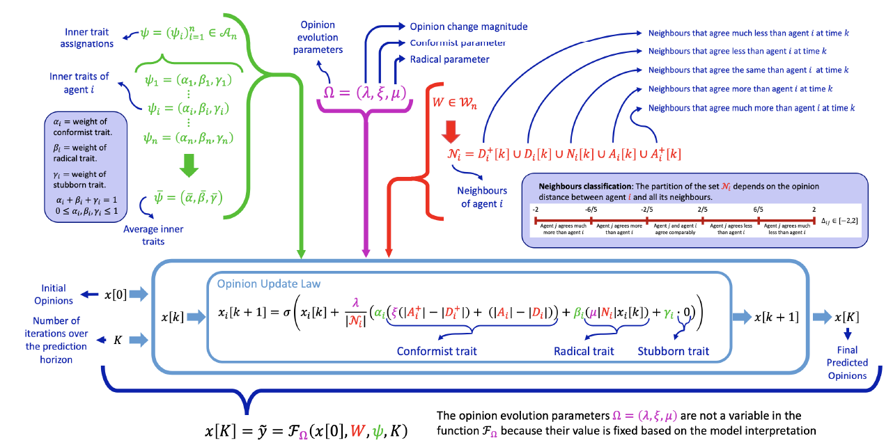
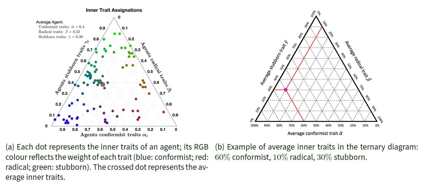
The overall behaviour of each agent results from the combination of three complementary inner traits: conformism, leading the agent to agree with its neighbours; radicalism, driving the agent to reinforce its opinion; and stubbornness, anchoring the agent to its current opinion. The conformism, radicalism and stubbornness degree of agent $i$ is respectively denoted by $\alpha_i$, $\beta_i$ and $\gamma_i$. The parameters $\psi_i = (\alpha_i,\beta_i,\gamma_i)$, quantifying the inner traits of agent $i$, satisfy $\alpha_i, \beta_i, \gamma_i\in[0,1]$ and $\alpha_i+\beta_i+\gamma_i = 1$ for all $i$. We call inner traits assignation the collection of inner traits of all agents, $\psi := (\psi_i )_{i\in V}$. The model features are summarised in Figure 2.

The opinion change $\Delta x_i[k]$ of agent $i$ at time $k$ is thus the convex combination of the behaviour of a purely conformist, purely radical, and purely stubborn agent,

\[ \Delta x_i[k] = \alpha_i f^\text{con}_i + \beta_i f^\text{rad}_i + \gamma_i f^\text{stb}_i,\]

\[(4)\]

with $f^\text{con}_i$, $f^\text{rad}_i$, and $f^\text{stb}_i$ taken as:

\[ f^\text{con}_i = \frac{\lambda}{|\mathcal{N}_i|}\Big( \xi|A^+_i| + |A_i| - |D_i| - \xi|D^+_i| \Big), \qquad f^\text{rad}_i = \frac{\lambda}{|\mathcal{N}_i|}\mu|N_i|x_i[k], \qquad f^\text{stb}_i = 0,\]

\[(5)\]

where $\lambda$, $\xi$, and $\mu$ are positive parameters: $\lambda$ weighs the overall opinion change magnitude, $\xi$ weighs the increased influence that neighbours with distant opinions have over conformist traits, and $\mu$ weighs the influence of the agent’s own opinion in radical traits. We call these opinion evolution parameters: $\Omega = (\lambda, \xi, \mu)$; see Figure 2.

To better understand Equations 5 and choose reasonable values for the parameters, one can think of how an extreme agent ($\alpha_i=1$, or $\beta_i=1$, or $\gamma_i=1$) behaves.

A purely conformist agent ($\alpha_i = 1$, $\beta_i=0$, $\gamma_i=0$) evolves towards an opinion comparable to that of its neighbours. For instance, if $N_i = \mathcal{N}_i$ (all the neighbours of agent $i$ agree comparably), then agent $i$ does not change its opinion. If $A_i = \mathcal{N}_i$ (all the neighbours of agent $i$ agree more), agent $i$ increases its opinion $x_i$ by $\lambda$; given that all the neighbours of agent $i$ are in the set $A_i$, a value $\lambda = 0.4$ guarantees that, if all the neighbour opinions remain unchanged, then at the next time step all the neighbours of agent $i$ will be in the set $N_i$, hence perceived as having a comparable opinion. Instead, if $A^+_i = \mathcal{N}_i$, then the opinion of agent $i$ needs to increase $0.8=2\lambda$ in order to be perceived as comparable to its neighbours’ at the next time step, and therefore a natural choice is $\xi=2$. The same reasoning can be applied to the sets $D_i$ and $D^+_i$.
A purely radical agent ($\alpha_i = 0$, $\beta_i=1$, $\gamma_i=0$) ignores neighbours with a different opinion and only cares about agents that think comparably to itself, hence it reinforces its current opinion $x_i[k]$ depending on the magnitude of its own opinion and on the fraction of its neighbours in the set $N_i$. To make sure that radical traits can affect the opinion change more strongly than conformist traits, we need $\mu>1$. In fact, if $\mu=1$, then $|f^\text{rad}_i|<|f^\text{con}_i|$ in general: the opinion change caused by the radical trait (which is proportional to $x_i[k]$, and $|x_i[k]|\leq1$) is smaller in magnitude than the one caused by the conformist trait. In our simulations, we set $\mu = 5$. The effect of different values of $\mu$ can be seen in Table 5.
A purely stubborn agent ($\alpha_i = 0$, $\beta_i=0$, $\gamma_i=1$) does not change its opinion under any circumstance.

The new opinion of agent $i$ at time $k+1$ is the sum of the previous opinion $x_i[k]$ and the opinion change $\Delta x_i[k]$, modulated by the saturation function $\sigma$

\[ \sigma(x) = \begin{cases} x &\text{if}\quad |x|\leq1 \\ \text{sign}(x) &\text{if}\quad |x|>1 \end{cases}\]

\[(6)\]

so as to guarantee that the opinions remain in the interval $[-1,1]$. The complete opinion update law is therefore:

\[ x_i[k+1] = \sigma\Bigg( x_i[k] + \frac{\lambda}{|\mathcal{N}_i|} \Big( \alpha_i\xi \big(|A^+_i| - |D^+_i|\big) + \alpha_i\big(|A_i| - |D_i|\big) + \beta_i\mu|N_i|x_i[k] \Big) \Bigg), \qquad \forall i\in V.\]

\[(7)\]

The opinions evolve, with simultaneous periodic updates at fixed discrete-time instants, according to Equation 7, which is fully deterministic: at each time step, every agent updates its opinion according to Equation 7, relying on the neighbour classification obtained through Equation 2. The parameter values and the signed digraph are constant and, once they are assigned, the model evolution is completely determined by the initial opinions.

The mathematical model formulation relies on four main assumptions: 1) opinions can be represented by real numbers in the [-1, 1] interval and agents update their opinions simultaneously over discrete time instants (standard assumptions for opinion formation models); 2) agents can either trust or mistrust the opinions they perceive from their neighbours, as reflected by the edge signs in the digraph (Altafini 2013; Xia et al. 2016); 3) agents cannot measure the opinion of their neighbours with infinite accuracy, but they can classify them according to their perceived opinions, through the classification mechanism in Equation 2; 4) the behaviour of each agent is the result of a combination of three psychological traits: conformism, radicalism, and stubbornness. These four assumptions, together with their mathematical representation in Equation 7, are the foundations for the proposed model.

Model parameters

The Classification-based (CB) model has three types of parameters: the signed digraph weights $w_{ij}$; the inner traits assignation $\psi_i = (\alpha_i,\beta_i,\gamma_i)$; and the opinion evolution parameters $\Omega = (\lambda, \xi, \mu)=(0.4,2,5)$ whose values are fixed, and chosen based on the model interpretation. Later, a parameter sensitivity analysis explores how the model evolution is affected by changes in opinion evolution parameters.

If the model has $n$ agents, then:

The signed digraph has weight matrix $W\in\mathcal{W}_n$. In general, $\mathcal{W}_n= \{-1,0,1\}^{n\times n}$, but we can focus for instance on small-world, or strongly connected, networks.

The inner traits assignation is $\psi\in\mathcal{A}_n$, where:

\[\mathcal{A}_n= \Big\{\psi= (\psi_i)_{i\in V} = \big((\alpha_i, \beta_i, \gamma_i)\big)_{i=1}^n\mid \alpha_i,\beta_i,\gamma_i\in[0,1] \quad \mbox{and} \quad \alpha_i+\beta_i+\gamma_i = 1, \quad \forall i\in V\Big\}.\]

\[(8)\]

We omit the subscript $n$ from the sets $\mathcal{W}$ and $\mathcal{A}$ for simplicity. Given $n$ agents, a signed digraph $W\in\mathcal{W}$, an inner traits assignation $\psi\in\mathcal{A}$, and a vector of initial opinions $x[0]$, the opinion formation model evolves according to Equation 7. The vector $x[K]$ of opinions after $K$ iterations can be explicitly represented as a function of $W$, $\psi$, and $x[0]$ by the map $\mathcal{F}_\Omega$ ($x[K]$ also depends on $\Omega$, whose value, given by the model interpretation, is fixed) as:

\[x[K] = \mathcal{F}_\Omega(x[0], W, \psi, K)\]

\[(9)\]

The value of $K$ depends on the type of statements and the prediction horizon. For statements related to core values or beliefs, opinions are not expected to change very fast and one could consider roughly 10 changes per year. Therefore, if the model is used to predict the opinions after 5 years, $K=50$. On the other hand, the opinions on more superficial topics could change faster and, over the same 5-year timespan, it could be $K=500$. See Figure 2 for a summary of the model parameters and features.

**Figure 2.** Visualisation of the model features and parameters. The model has three parameter types: inner traits assignation $\psi$ (in green), opinion evolution parameters $\Omega$ (in magenta), and signed digraph weights $W$ (in red). These parameters appear in the Opinion Update Law of Equation 7, which is a convex combination of contributions by conformist, radical, and stubborn traits, with the opinions of neighbouring agents evaluated through a classification-based approach. Given the initial conditions $x[0]$ and the number $K$ of iterations over the prediction horizon, the Opinion Update Law produces the final predicted opinions $\tilde{y} = x[K]$. The opinion evolution parameters $\Omega$ can be fixed based on the model interpretation. Then, the final predicted opinions in each particular case are a function $x[K] = \mathcal{F}_\Omega(x[0], W, \psi, K)$ of the chosen initial opinions, signed digraph weights, inner traits assignation, and number of iterations in the prediction horizon.

To validate the model – namely, assess its potential to closely reproduce the evolution of opinions in real life with suitably chosen parameters – we consider real initial and final opinions, denoted by $x$ and $y$ respectively, taken from survey data. Assuming that $y$ are the real opinions $K$ iterations after the real initial opinions $x$, these data can be used to find values of the model parameters (edge weights $W$ and inner traits $\psi$) that produce opinions that match as closely as possible the real opinion evolution, through the minimisation problem:

\[ (\widehat{W}, \widehat{\psi}) = \mathop{\mathrm{arg\,min}}_{\substack{W\in\mathcal{W}\\ \psi\in\mathcal{A}}}J(y,\tilde{y}) \qquad \mbox{such that} \qquad \tilde{y} = \mathcal{F}_\Omega(x, W, \psi, K),\]

\[(10)\]

where the cost function $J(y,\tilde{y})$, described and explained in Equation 16, quantifies the mismatch between opinion vectors $y$ and $\tilde{y}$.

If the same population is asked to quantify the agreement with $Q$ different statements, the signed digraph cannot change. However, the inner traits assignation can vary depending on the statement, since each individual may have different attitudes towards different topics. Therefore, if $\psi^{(l)}$ represents the inner traits assignation associated with statement $l$, values for the parameters $W$ and $(\psi^{(l)})_{l=1}^Q$ that produce predicted opinions as similar as possible to the real ones can be found through the free optimisation problem

\[ \big(\widehat{W}, (\widehat{\psi^{(l)}})_{l=1}^Q\big) = \mathop{\mathrm{arg\,min}}_{\substack{W\in\mathcal{W}\\ \psi^{(l)}\in\mathcal{A}}} \sum_{l=1}^QJ(y_l,\tilde{y}_l) \qquad\qquad \tilde{y}_l= \mathcal{F}_\Omega(x_l, W, \psi^{(l)}, K)\]

\[(11)\]

where $x_l$ and $y_l$ are the known initial and final opinions related to statement $l$.

If instead all the inner traits assignations are constrained to be the same for every question, we consider the constrained optimisation problem:

\[ (\widehat{W}, \widehat{\psi}) = \mathop{\mathrm{arg\,min}}_{\substack{W\in\mathcal{W}\\ \psi\in\mathcal{A}}} \sum_{l=1}^QJ(y_l,\tilde{y}_l) \qquad\qquad \tilde{y}_l= \mathcal{F}_\Omega(x_l, W, \psi, K)\]

\[(12)\]

The free optimisation problem, where the inner assignations can change, allows for a more thorough study of the behaviour of a population, while the constrained optimisation problem allows for a more rigorous testing of the prediction capabilities of the model in the form of cross-validation: the answers to some questions can be used as training datasets to choose the model parameters, and the model performance can then be tested on the remaining questions.

Simulation Results

To gain insight into the Classification-based (CB) model, this section presents four different types of simulation results: 1) Simulations in Simple Cases evolve the model in simple, special cases to gain intuition into its behaviour; 2) Parameter Sensitivity Analysis studies how changes in each of the model parameters (inner traits assignation, signed digraph, opinion evolution parameters) affect the model behaviour; 3) Characterisation of Model Outcomes uses distributional measures, including the recently proposed Bias, Diversity, and Fragmentation (Lorenz et al. 2021), to characterise the variety of opinion vectors that the Classification-based model can produce; 4) Model Validation with Real Data leverages real data from the WVS to show that the CB model has the potential to reproduce the time evolution of real opinions in society (with parameters chosen through the free and the constrained optimisation problems of Equations 11 and 12 respectively).
Due to the deterministic nature of the model, running it with the same initial opinions, parameters, and interconnection network always produces the same results. Given a parameter choice and a network, the model evolution can only change due to different initial conditions (see the repeated model runs in Figure 5).

To facilitate the interpretation of simulation results, we introduce some definitions. Given the inner traits assignation $\psi= (\psi_i)_{i\in V} = \big( (\alpha_i,\beta_i,\gamma_i) \big)_{i\in V}$, the associated average inner traits

\[\bar{\psi} = (\bar{\alpha}, \bar{\beta}, \bar{\gamma}) \quad \text{where} \quad \bar{\alpha} = \frac{1}{n}\sum_{i\in V}\alpha_i \qquad \bar{\beta} = \frac{1}{n}\sum_{i\in V}\beta_i \qquad \bar{\gamma} = \frac{1}{n}\sum_{i\in V}\gamma_i,\]

\[(13)\]

represent the traits of an average agent in the considered society or population with $n = |V|$ agents. Inner traits assignation $\psi$ and the corresponding average inner traits $\bar{\psi}$ can be plotted in a ternary diagram as shown in Figure 3a (the ternary plots were made using modified scripts from Sandrock 2012). Figure 3b explains how to interpret a point in the ternary diagram.

**Figure 3.** Ternary diagrams visualising inner traits assignations $\psi$ and average inner traits $\bar{\psi}$. Panel (a) shows the whole inner traits assignation, with each dot corresponding to the traits of a singe agent, along with the average inner traits (crossed dot). Panel (b) only shows the average inner traits of a complete population (magenta dot).

The general agreement of an opinion vector $x = (x_i)_{i=1}^n$, quantified by the pair $(\theta_+, \theta_-)$ where

\[ \theta_- = \sum_{x_i<0}x_i \qquad \mbox{and} \qquad \theta_+ = \sum_{x_i>0}x_i,\]

\[(14)\]

and can be interpreted as the overall level of agreement and disagreement in the whole society.

All the simulations involve a population of $n=100$ agents. All the digraphs used in both Parameter Sensitivity Analysis and Model Validation with Real Data have a small-world network topology, with an assigned probability for positive and negative edges, and are strongly connected. We consider small-world networks because they have a high clustering coefficient (neighbours of neighbours of agent $i$ are likely also neighbours of agent $i$) and low diameter (maximum distance between two agents of the network), which are believed to be characteristics of real-life social networks (Elgazzar 2003; Watts & Strogatz 1998). The directed small-world networks were built based on the Watts-Strogatz algorithm. Appendix D describes the computation of network metrics. The signed digraphs are not restricted to be structurally balanced, to account for the fact that also non-structurally-balanced networks have been considered in the literature when modelling social dynamics (Estrada 2019; Leinhardt 1977; Opp 1984).

In all the considered simulations, the initial opinions, traits and networks are assigned independently. A different approach – which is left for future work – could be to assign them in some correlated way: e.g., initial opinions and network could be correlated by assigning the initial opinions such that two vertices connected by an edge have a very similar (or very distant) initial opinion; traits and network could be correlated by assigning the agent parameters with a probability that depends on the corresponding vertex characteristics, for example assuming that vertices with higher out-degree have a higher probability of being completely conformist, or radical. Correlations between initial opinions, traits, and network characteristics can reproduce different types of societies present in real life (for instance, in a society that values tradition, highly stubborn agents may be more influential than others, and hence the corresponding vertices may have a higher out-degree).

Simulations in simple cases

To better understand the model behaviour, we simulate the model evolution in special simple cases. First, for the same digraph with a lattice topology, we vary the inner traits assignations (Figure 4). Then, for the same inner traits assignation, we consider different digraph topologies (complete, lattice, ring, small-world) and different, randomly chosen, initial opinions (Figure 5).

Different inner traits assignations

We consider a signed lattice digraph, where each agent has 4 in-neighbours and the edges are positive with probability $0.77$. All the agents have the same inner traits, combining only two inner traits: stubbornness and radicalism; radicalism and conformism; conformism and stubbornness. Starting from the same initial opinions (which are discrete, and hence the plot with purely stubborn agents shows evenly distributed horizontal lines), Figure 4 shows the opinion evolution over 30 time steps.

**Figure 4.** Evolution of the CB model, starting from the same initial opinions, over a signed lattice digraph where the edges are positive with probability $0.77$. In each simulation, all $100$ agents have the same inner traits that are a combination of only two of the possible traits: stubbornness (Stb), radicalism (Rad), and conformism (Con). The top labels show the proportion of each trait: the upper left (respectively, right) graph corresponds to a simulation where all agents are purely stubborn (resp. radical). The colour of the lines is the RGB representation of the inner traits assignations (blue: conformist; red: radical; green: stubborn).

Figure 4 shows that Radicalism tends to form polarisation by driving the agents to extreme opposite views. Conformism tends to create consensus; however, because of the classification approach, the agents do not converge to the very same opinion (close enough agents are unable to perceive their opinion difference, because opinions are assessed with finite resolution). Stubbornness slows down the effect of the other two traits; only in a fully stubborn population everyone keeps its initial opinion. Among the three traits, radicalism appears to have the greatest effect: even a small amount of radicalism can prevent conformism from forming consensus (as seen in the 10-90 Rad-Con plot), and can yield polarisation in a very stubborn society (as seen in the 90-10 Stb-Rad plot).

Different digraph topologies

Additional intuition on the model behaviour can be gained by studying the effect of different initial opinions and different digraph topologies with fixed inner trait parameters. Figure 5 shows 10 simulations starting from various, randomly chosen, initial opinions and evolved over four signed digraphs with Complete, Lattice, Ring, and Small-World topologies. The inner traits assignation for all these simulations is kept constant and is shown in Figure 3a.

Both the digraph topology (dictating how the agents communicate among them) and the initial opinions (providing the starting point of the evolution) have a significant effect on the opinion evolution and the final predicted opinions. For Lattice and Ring digraphs, there is a clear tendency towards consensus at one extreme opinion (completely agree or completely disagree), even when, as in this case, the average radical trait is relatively low. A possible explanation is that in both these topologies agents have less in-neighbours, so the radical trait can have a stronger effect. Another possible explanation is that both these types of networks have a larger average path length, and diameter, than Complete and Small-World networks, and therefore the ‘consensus effect’ takes more time to act than in more connected networks.

Indeed, since they share common features, the Complete and Small-World digraphs (small diameter), as well as the Lattice and Ring digraphs (large diameter), showcase similar behaviours and similar final opinion distributions, across all the chosen initial opinion distributions. We have observed that this tendency is recurrent for several different choices of inner traits assignations.

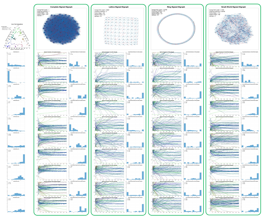
**Figure 5.** Evolution of the CB model, with 100 agents, over four different digraph topologies and starting from ten different, randomly chosen, initial opinions, shown on the left-most column. Each of the four columns framed in green shows the opinion evolution and the final opinion distribution for each of the initial opinions, for a different choice of the digraph (Complete, Lattice, Ring, Small-World), shown at the top of the column along with its metrics. The inner traits assignation is presented at the top left and has average traits: $\overline{\alpha} = 0.4$ (conformist), $\overline{\beta} = 0.22$ (radical), and $\overline{\gamma} = 0.38$ (stubborn). The ternary diagram of these inner traits can also be seen in Figure 3a.

As is apparent from Figure 4, the inner traits assignation has a tremendous effect on the opinion evolution. The simulations of Figure 5 reinforce this idea by showing that, although the initial opinions and digraph topology do have an impact, keeping the same inner traits assignation restricts the final opinion distributions to some characteristic patterns.

Parameter sensitivity analysis

We select a set of nominal parameters (which, for given initial conditions, produce nominal simulation results) as a baseline with which other parameter choices can be compared. We choose a nominal inner traits assignation that leads to model outcomes that closely reproduce real data from the World Values Survey (in fact, it is close to some of the inner traits assignations resulting from the Free optimisation problem 10, see Figure 19a), and therefore has the potential to represent a realistic society; moreover, it allows us to showcase the wide range of different opinion evolutions that the model can produce. Then, we vary inner traits assignations, signed digraph and opinion evolution parameters, one by one, and study their effect on the simulated behaviour.

Nominal parameters and nominal results

We consider the initial opinions shown in Figure 6a, which evolve according to the model with the nominal parameters: $\lambda = 0.4$, $\xi= 2$, $\mu = 5$, inner traits assignations in Figure 6b, and signed digraph in Figure 6c.

**Figure 6.** Initial opinions and nominal parameters.

The initial opinions shown in Figure 6a have $\theta_- = -19.3$ and $\theta_+ = 41.5$, indicating a strong general agreement since $\theta_+>-\theta_-$. Figure 6b shows that most agents have very strong conformist traits, with a notable percentage of radicalism, resulting in an average agent (crossed dot) with $60\%$ conformist traits, $30\%$ radical traits, and $10\%$ stubborn traits. The nominal signed digraph in Figure 6c is highly connected, with average path length $2.12$, clustering coefficient $0.38$, diameter $4$. It has $834$ positive edges and $767$ negative edges.

The nominal results are shown in Figure 7. Figure 7a shows the opinion evolution of every agent. The line colour represents the percentage of conformist, radical, and stubborn agent traits (blue for conformist, red for radical, and green for stubborn). The purple colour of most lines corresponds to a combination of conformist and radical traits. The discontinuity in the opinion change is due to the classification process leading to a discontinuous opinion update law. The opinion evolution of the various agents shows a great variability in opinion changes, without a clear global tendency.

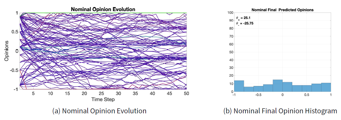
**Figure 7.** Simulation results with the nominal parameter values (evolving 100 agents).

Figure 7b shows the histogram of the nominal final opinions predicted by the model after 50 time steps. Compared with the initial opinions, the final opinions appear to have a more uniform distribution: in fact, for the nominal final opinions, $\theta_- = -25.75$ and $\theta_+ = 25.1$, hence $\theta_+ \approx -\theta_-$. The behaviour of the opinion evolution and the distribution of the final opinions is explained by the presence of two opposing forces that drive the opinion of all the agents: on one hand, the tendency to achieve consensus, due to the conformist traits, drives the agents towards the centre; on the other hand, the radical traits move the opinions towards extreme values.

Varying the inner traits assignations $\psi$

To evaluate the effect of different inner traits assignations, we change the nominal inner traits assignations of Figure 6b and simulate the opinion evolution, keeping all the other parameters unchanged. The two new inner traits assignations, shown in Figures 8a and 8d, are simply rotations of the nominal inner traits assignations. The corresponding opinion evolutions are shown in Figures 8b and 8e, while the final opinion histograms are presented in Figures 8c and 8f.

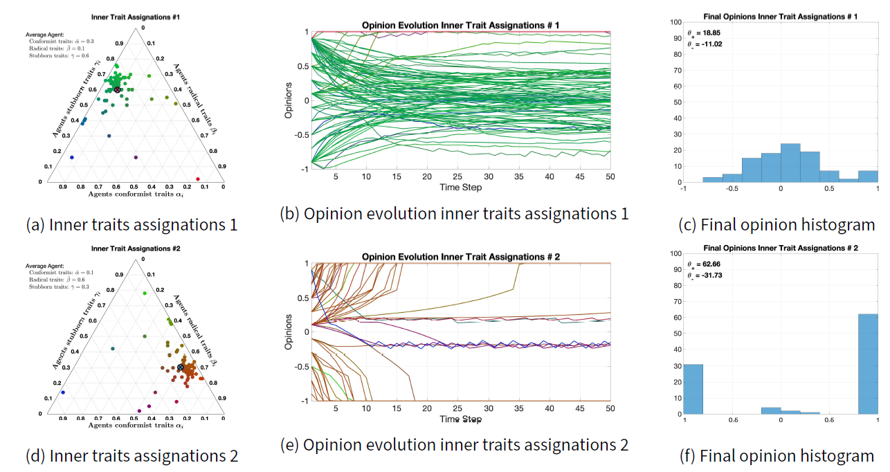
**Figure 8.** Effect of changing the inner traits assignations (evolving 100 agents).

Comparing the opinion evolutions of Figures 7a, 8b, and 8e and the final opinion histograms of Figures 7b, 8c, and 8f reveals the profound effect of different inner traits assignations on the opinion evolution. In the inner traits assignation of Figure 8a, the agents are mostly stubborn and conformist. This results in a very slow convergence towards the mean, driven by conformist traits and slowed down by stubborn traits. Because of the neighbour classification mechanism, even completely conformist agents would not reach perfect consensus, but would rather converge to an opinion subinterval where all the agents perceive that the others have a comparable opinion. This tendency towards the mean can be seen in the final opinion histogram of Figure 8c, where both $\theta_- = -11.02$ and $\theta_+ = 18.85$ are much closer to 0 than the final opinions in Figure 7b.

On the other hand, the inner traits assignation of Figure 8d gives agents pronounced radical traits. Both the opinion evolution in Figure 8e and the final opinion histogram in Figure 8f show that agents lean towards extreme opinions. A bunch of agents keeps its opinion closer to zero. The line colours (closer to blue and green) show that these agents do not have very strong radical traits, and instead they are more conformist and stubborn: such traits allow these agents to avoid extreme opinions.

Varying the signed digraph $W$

To study the effect of changing the signs of the weights of the signed digraph, the nominal signed digraph of Figure 6c is modified into the signed digraphs shown in Figures 9a and 9d. The topology is unchanged, but the number of positive and negative edges is changed. The resulting opinion evolution and final opinion histograms are shown in Figures 9b and 9e, and in Figures 9c and 9f respectively.

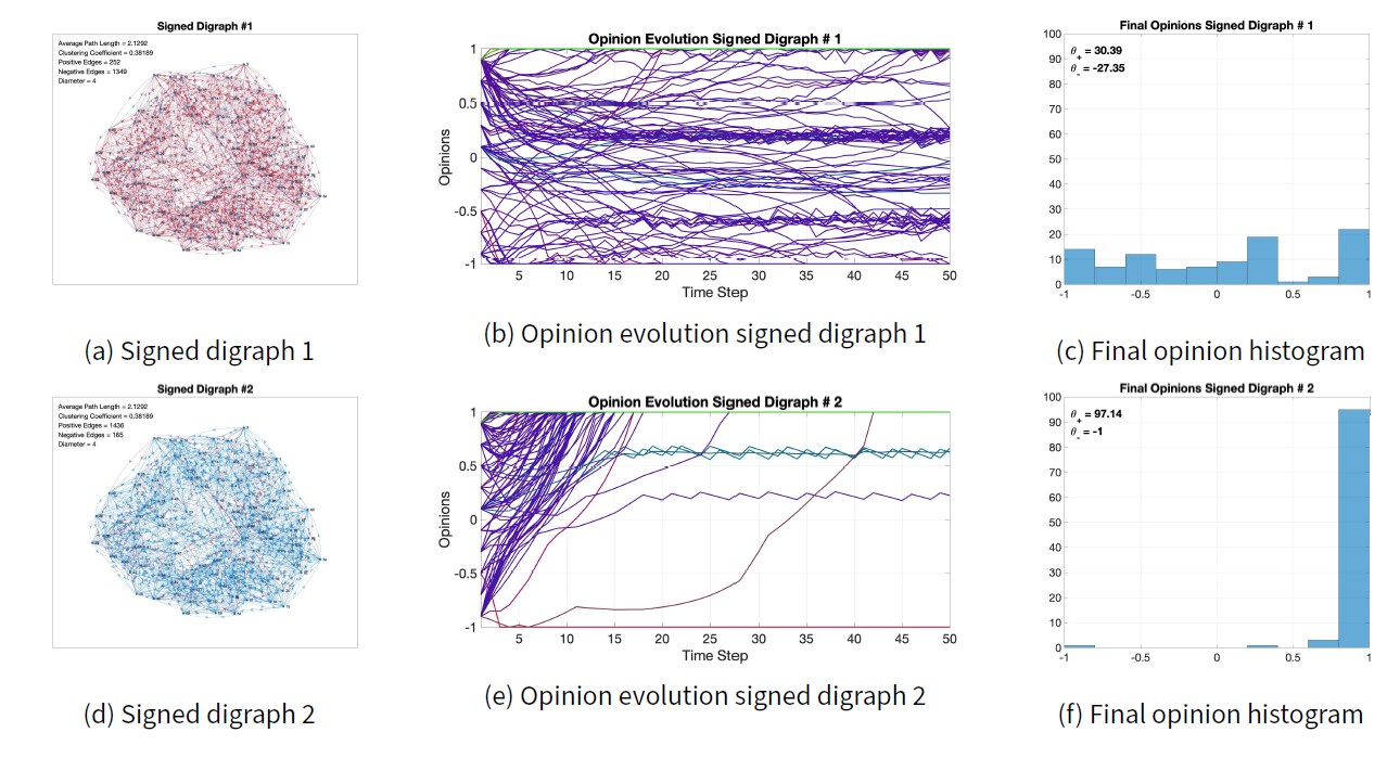
**Figure 9.** Effect of changing the signed digraph (evolving 100 agents).

Compared with the nominal results in Figures 7a and 7b, the most different outcome occurs when most edges are positive (digraph in Figure 9d). In this case, the end result is almost perfect consensus for the $+1$ opinion, because the initial opinion, with $\theta_- = -19.3$ and $\theta_+ = 41.5$, is more skewed towards $+1$. The presence of negative edges is crucial to avoid trivial consensus outcomes even when the agents are not completely conformist. The opinion evolution in Figure 9e shows that, initially, conformist traits pull the opinions towards positive values, and then radical traits make them increase in value until they reach $+1$. Purely radical agents would have produced polarisation instead of consensus.

When increasing the number of negative edges (digraph in Figure 9a), the final opinions in Figure 9c are different from the nominal ones, but the qualitative behaviour is comparable.

Varying the opinion evolution parameters $\Omega$

We study the sensitivity with respect to the opinion evolution parameters $\Omega = (\lambda, \xi, \mu)$, where: $\lambda$ is the overall opinion change magnitude, and can also be thought of as a time scaling parameter; $\xi$ gives more weight to distant opinions for conformist traits; $\mu$ increases the opinion change for radical traits. We change these parameters one at the time, with respect to the nominal parameters, and compare the results with the nominal results in Figure 7.

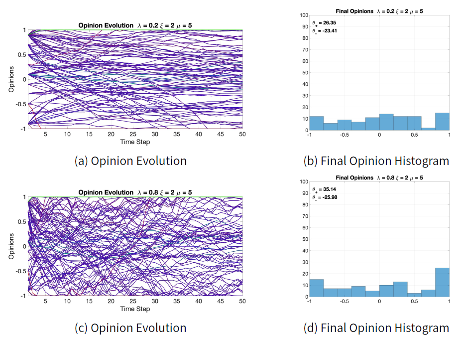
Figure 10 shows the opinion evolution and final histogram for $\lambda = 0.2$ and $\lambda = 0.8$. The final histograms in Figures 10b and 10d do not change much with respect to the nominal. The most significant change can be noticed in Figures 10a and 10c, showing that indeed a higher value of $\lambda$ produces larger changes in the opinions. Overall, however, the effect of varying $\lambda$ is very limited.

**Figure 10.** Effect of changing $\lambda$ from the nominal value $\lambda = 0.4$ to $\lambda = 0.2$ (Figures 10a and 10b) and $\lambda = 0.8$ (Figures 10 c and 10 d) evolving 100 agents.

The effect of varying $\xi$ is shown in Figure 11. The changes in both the opinion evolution and the final opinion histogram are quite noticeable. A value of $\xi=1$ means that distant opinions have the same attracting power as closer opinions for the conformist traits, hence in general the conformist trait has less influence over the whole opinion change, which is instead dominated by the radical traits. The result is visible in the opinion evolution in Figure 11a and the final opinion histogram in Figure 11b. On the contrary, increasing the value to $\xi=4$ yields a stronger conformist tendency towards consensus, evident when comparing the nominal final opinions in Figure 7b with the final opinions with $\xi=4$ in Figure 11d, and the respective $\theta_-$ and $\theta_+$.

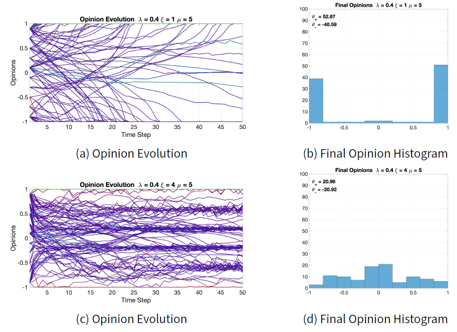
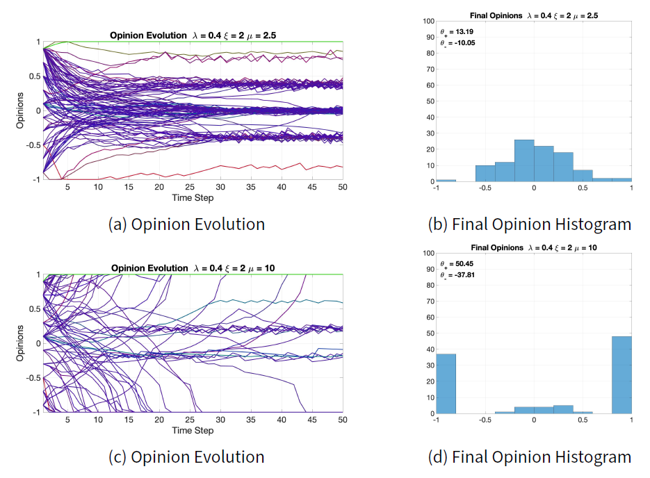
**Figure 11.** Effect of changing $\xi$ from the nominal value $\xi = 2$ to $\xi = 1$ (Figures 11 a and 11 b) and $\xi = 0.8$ (Figures 11 c and 11 d) evolving 100 agents.

Parameter $\mu$ modulates the effect of radical traits on the opinion evolution. Comparing Figure 12b with Figure 12d shows that a larger $\mu$ increases radicalism in the population, which leads to polarisation for the given initial opinions. A similar effect is achieved by varying $\xi$: in fact, both $\xi$ and $\mu$ affect the balance between the conformist tendency towards consensus and the radical tendency towards polarisation. Although both $\xi$ and $\mu$ play a role in the conformist-radical balance, they are not completely complementary: an increase in $\xi$ is not equivalent to a decrease in $\mu$. This can be seen by comparing Figures 11d and 12b: increasing $\xi$ produces final opinions that are more evenly distributed than those obtained by decreasing $\mu$. Moreover, increasing radicalism does not always lead to polarisation: this happens only when the opinions have both positive and negative values. If the opinions have only positive values or only negative values, then radicalism will move all of them to a single extreme, resulting in consensus. Therefore, it is not possible to generalise the idea that more radicalism always leads to polarisation, regardless of the initial opinions.

**Figure 12.** Effect of changing $\mu$ from the nominal value $\mu = 5$ to $\mu = 2.5$ (Figures 12a and 12b) and $\mu = 10$ (Figures 12c and 12d) evolving 100 agents.

Characterisation of model outcomes

We characterise the model outcomes using different distributional measures: first, Bias, Diversity, and Fragmentation of the opinion distributions, recently proposed by Lorenz et al. (2021), to relate the inner trait assignations with qualitative properties of the model; then, plots of the mean and of the mean of the absolute values of the final opinion distributions that the model can generate.

Bias, Diversity, and Fragmentation analysis

Recently, Lorenz et al. (2021) have proposed Bias, Diversity, and Fragmentation as measures to analyse opinion formation models: Bias is the deviation of the mean opinion from the neutral opinion (indifference), Diversity is the normalised standard deviation of opinions, and Fragmentation measures how uneven the histogram of a given opinion distribution is. Their values range from 0 to 1; details are in Appendix F.

Figures 13a and 13e show the histograms of two different initial opinion distributions and their Bias, Diversity, Fragmentation values. In both cases, Bias is very low because the mean of opinions is almost zero. Figure 13a has a higher Fragmentation than Figure 13e, because Figure 13a shows two subgroups, whereas Figure 13e only one. Figure 13a has a higher Diversity than Figure 13e, because the two subgroups in Figure 13a are located at opposite sides.

Given a signed digraph $W$ and inner trait assignations $\psi$, we evolve the model starting from the chosen initial opinions, and compute Bias, Diversity, and Fragmentation for the resulting final opinion distribution. To investigate how the inner traits affect Bias, Diversity, and Fragmentation, we evolve each of the initial opinions in Figure 13a and Figure 13e for 50 time steps, over the same constant signed digraph $W$ (with Small-World network topology, see Figure 16a), with each of the inner trait assignations $\psi$ in the set $\Upsilon$, defined as:

\[\Upsilon = \Big\{\psi= (\psi_i)_{i\in V} = \big((\alpha, \beta, \gamma)\big)_{i=1}^n\mid \alpha,\beta,\gamma\in\{0, 0.05, 0.1, \dots, 0.9, 0.95, 1\} \quad \mbox{and} \quad \alpha+\beta+\gamma = 1\Big\}.\]

\[(15)\]

The set $\Upsilon$ contains 231 different inner trait assignations where all the agents have the same inner traits. Evolving the initial opinions for each of the inner trait assignations in $\Upsilon$ for 50 time steps results in 231 final opinions. For all these final opinions, Bias, Diversity, and Fragmentation are computed and shown in ternary diagrams as heat maps. Figures 13b, 13c, 13d (respectively, 13f, 13g, 13h) show the resulting ternary diagrams for the initial opinions in Figure 13a (resp. 13e).

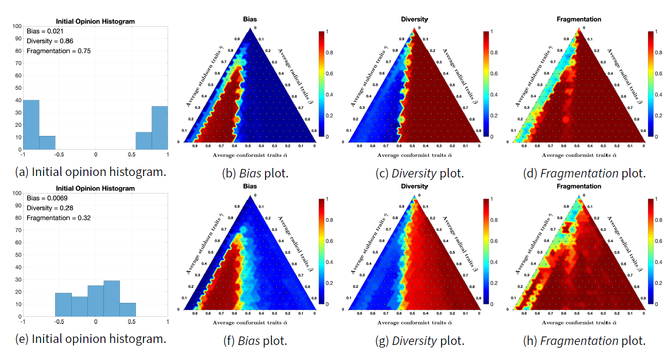
**Figure 13.** Bias, Diversity and Fragmentation ternary plots for the initial opinions shown to the left. All opinions evolve for 50 time steps over the signed digraph shown in Figure 16a. All simulations are for 100 agents.

Interestingly, although the initial opinions are different, the resulting ternary diagrams are relatively similar. Bias is very low, except when the average radical trait is in the range 0.1-0.3 and the average stubborn trait is below 0.7; in fact, when the radical trait is high, agents tend to move to extremes and, if there is a comparable number of agents with positive and negative opinions (as in this case, for both initial opinions), the Bias will be near zero. On the other hand, when the conformist trait dominates, it moves opinions towards the mean, which in this case is also near zero. High Bias is achieved only when there is an appropriate combination of conformist and radical traits that moves agents from one half of the opinion interval to the other.Diversity and Fragmentation are almost 1 (the highest possible value) for medium to high levels of radicalism, because agents move to extremes.

Figure 14 shows simulation results analogous to the ones presented in Figure 13, but for an initial opinion distribution having higher Bias. In this case, because more agents have a positive opinion, the radical trait moves more agents towards the extreme opinion $1$, resulting in turn in a higher Bias and lower Diversity for the final opinions (which, in many cases, are 1 for almost all agents). Fragmentation is still very high, since there is significant concentration of agents around opinion $1$.

**Figure 14.** Bias, Diversity and Fragmentation ternary plots for the initial opinions shown to the left. All opinions evolve for 50 time steps over the signed digraph shown in Figure 16a. All simulations are for 100 agents.

The results in Figure 14b can also be visualised by plotting in a Cartesian plane the initial Bias on the $x$-axis and the final Bias on the $y$-axis for the 231 simulations. The result is a plot with 231 points of different colour. The colour of each point in the Cartesian plane is the RGB representation of the inner traits assignations (blue: conformist; red: radical; green: stubborn) associated with the corresponding simulation. Since all the simulations start from the same initial opinions (for instance, those shown in Figure 14a), all the points have the same $x$-coordinate. This allows for several Bias ternary plots to be represented in the same figure, providing an overall visualisation of how the final Bias relates to the initial Bias for different inner trait assignations. Such a plot is shown in Figure 15a for 231 different initial opinions. Analogous plots for Diversity and Fragmentation are reported in Figures 15b and 15c respectively.

Figure 15a shows that the CB model cannot produce opinions with a Bias below 1.7 unless the initial Bias is below 1.7; this may happen because Bias is low when the opinions are either all close to 0 or partitioned in comparable agreement/disagreement groups (see Table 12 in Appendix F), and the classification algorithm prevents opinions from converging very close to 0. Figure 15b shows that the CB model can produce low Diversity for almost any initial opinion, primarily due to the conformist trait (prevalence of blue dots) that pushes agents towards the same opinion, thus decreasing Diversity. Higher Diversity is mostly due to the radical trait (prevalence of red dots). Figure 15c shows that the CB model can produce final opinions with a wide range of Fragmentation values, which are however quantised because they are computed based on histogram counts (instead of on the exact agent opinions). Red dots are present, but covered by other dots, suggesting a high concentration of dots in some areas of this plot. The green diagonal lines in Figures 15a, 15b, 15c corresponds to agents that are all completely stubborn, and therefore do not change opinion.

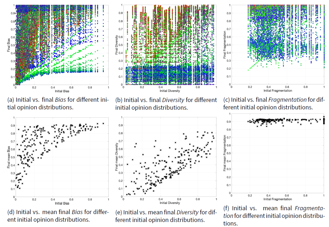
**Figure 15.** Initial vs. (mean) final Bias, Diversity, and Fragmentation. In the first row, the colour of each point represents the inner trait assignation of the corresponding agents. All opinions evolve for 50 time steps over the signed digraph shown in Figure 16a. All simulations are for 100 agents.

When plotting the initial Bias and the mean final Bias (averaged over all the 231 elements in $\Upsilon$), the 231 points with the same $x$-coordinate become a single point, as shown in Figure 15d. The same can be done for Diversity and Fragmentation, shown in Figures 15e and 15f. Collectively, these results provide further insight into the behaviour of the CB model. Figure 15d shows that the mean final Bias is always higher than the initial Bias. Figure 15e shows that there is an almost linear relation between the initial Diversity and the mean final Diversity. Figure 15f shows that the mean final Fragmentation is always near $1$, most likely due to the radical traits that move opinions to the extreme even if their weight is not particularly large (as seen in Figure 4).

Mean of opinions and opinion absolute values

The mean of the opinions, $\overline{x}$, and the mean of the opinions’ absolute values, $\overline{|x|}$, are other interesting metrics. The mean of the opinions has a clear meaning; the mean of the opinions’ absolute values represents the average level of interest the agents have in the considered statement. If $\overline{|x|}\approx0$, then most opinions are near $0$ (indifference); if $\overline{|x|}\approx1$, then most opinions are extreme, either complete disagreement $-1$ or complete agreement $1$ (high level of interest in the subject). The point $p(x) = (\overline{|x|}, \overline{x})$ in the Cartesian plane is located in the triangle with vertices $(0,0)$, $(1,-1)$, $(1,1)$. If $p(x)$ is near the origin, then most opinions are near zero; if $p(x)$ is located along the lines $y=\pm x$, then either all agents agree or all agents disagree with the same strength; if $p(x)$ is located near the line $x=1$, then most agents have extreme opinions; and if $p(x)$ is located near the point $(1,0)$, then the population is highly polarised.

Starting from an initial opinion distribution $x_o$, keeping the signed digraph $W$ constant, we evolve the model for different inner trait assignations. For each of the resulting opinion distributions $x_f$, we compute the corresponding point $p(x_f)$ and we plot all these points in the Cartesian plane, to show which opinion distributions the model can produce starting from the initial opinion distribution $x_o$. The point colour encodes the average inner traits, to visualise how the inner traits affect the resulting opinion distributions. This type of plot is shown in Figure 16 for three different initial opinion distributions (shown in the crossed dot) that evolved over two different Small-World signed digraphs, for all the inner trait assignations in the set $\tilde{\mathcal{A}}$ described in Appendix C. Plots along the same row evolve over the same signed digraph shown to the left. Plots along the same column have the same initial opinion distribution, represented by the crossed dot.

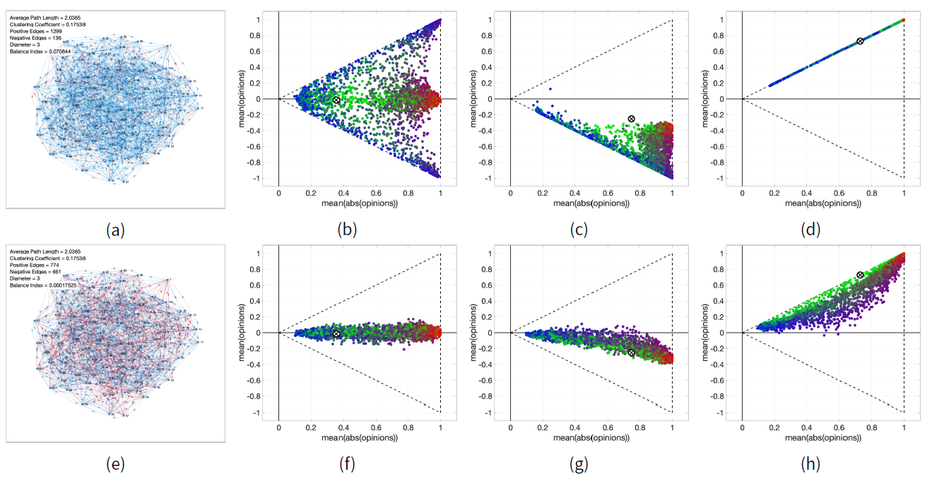
**Figure 16.** Plots of $\overline{x}$ and $\overline{|x|}$ starting from given initial opinion distributions (associated with the crossed dot) that are evolved, for 50 time steps, over the signed digraphs shown to the left, with inner agent parameters in the set $\tilde{\mathcal{A}}$ (described in Appendix F). The colour of each dot encodes the corresponding inner trait assignation. All simulations are for 100 agents.

The signed digraphs in Figures 16a and 16e have the same topology, but a different fraction of negative edges (9.47% in Figure 16a and 46.06% in Figure 16e). Comparing the evolution from the same initial opinions over the two different digraphs (Figures 16b vs. 16f; Figures 16c vs. 16g; Figures 16d vs. 16h) shows the significant effect the proportion of negative edges has on the system evolution. When most edges are positive, opinions reinforce themselves and the final opinions tends to move to extremes. When there are more negative edges, the digraph contains more unbalanced cycles (closed directed paths where the number of negative edges is odd) and therefore opinions tend to zero (as it happens in the Altafini model; Altafini (2013)). The initial opinion distribution also has a critical effect on the opinions that the model can produce: when the initial opinions have a significant non-zero mean, either positive or negative, the mean of the predicted opinions typically has the same sign (see Figures 16c, 16 d, 16g, and 16h). Only initial opinions whose mean is near zero can produce an equal amount of final opinions with positive and negative mean (see Figures 16b and 16f).

Overall, the plots shown in Figure 16 indicate that the Classification-based model is very flexible and can produce a rich variety of final opinion distributions.

Model validation with real data

Data from the World Values Survey are used to validate the CB model, by showing that, with a suitable choice of the parameters, the model can produce opinion evolutions similar to those observed in real societies. The World Values Survey is an international organisation that conducts surveys about ethics and values in different countries around the globe. These surveys are repeated every 5 years. We considered the answers to 30 questions, shown in Table 14, in 26 countries, shown in Table 13, in Appendix G. In each question, the respondents are asked to state the extent to which they agree with a statement in a Likert-scale 10. The answers given in the surveys of wave 5 are taken as initial opinions, while the answers of wave 6 are taken as final opinions. Details on the solution of the optimisation problems are provided in Appendix E.

Two minimisation problems are stated to find model parameters that produce predicted opinions similar to the ones found in the survey answers. The Free Optimisation Problem allows the inner traits assignation to change with questions; in the Constrained Optimisation Problem, the inner traits are fixed for all questions.

Given real and model-generated opinion vectors $r$ and $y$, for a population of $n$ agents, the cost function $J$ used in the minimisation problems 10, 11, and 12 is defined as

\[ J(r,y) = \sum_{i = 1}^n| \tilde{r}_i - \tilde{y}_i |,\]

\[(16)\]

where $\tilde{r} = (\tilde{r}_i)_{i=1}^n$ is the vector $\hat{r} = (\hat{r}_i)_{i=1}^n$ sorted in descending order, and $\hat{\cdot}$ is the quantisation function

\[\hat{r}_i = \mathop{\mathrm{arg\,min}}_{\zeta \in \mathcal{R}}\{|\zeta - r_i|\} \qquad \forall i = 1,\dots , n,\]

\[(17)\]

with $\mathcal{R}$ defined as $\mathcal{R}= \Big\{ \frac{1}{2}(u_k + u_{k+1}) \mid u_k = -1 + k\frac{2}{10} \quad k = 1, \dots , 9 \Big\}$. Quantisation is needed because the World Values Survey answers we consider as real opinions use a Likert scale 10: participants could choose their opinion from 10 different options. These opinions rescaled to be between -1 and 1 produce the set $\mathcal{R}$ and, therefore, the predicted opinions also need to be quantified in the same way. Both opinion vectors (real and predicted) are sorted in descending order, so that equal opinions add a zero to the total cost.

Even for a relatively small population $n= 100$, the size of the sets $\mathcal{W}$ (underlying signed digraph structures) and $\mathcal{A}$ (inner traits assignations) is enormous. Given the tremendous size of the parameter space $\mathcal{W}\times\mathcal{A}$, performing the minimisation over all possible signed digraphs and agent inner traits would be computationally intractable. Therefore, the minimisation occurs over small subsets $\tilde{\mathcal{W}}\subset\mathcal{W}$, $\tilde{\mathcal{A}}\subset\mathcal{A}$ of the whole parameter space. As a consequence, there is no guarantee that we are estimating the real parameter values or making the absolute best parameter choice: with other parameter choices, not included in $\tilde{\mathcal{W}}\times\tilde{\mathcal{A}}$, the model could reproduce the data with even better accuracy. Appendix C describes in detail the sets $\tilde{\mathcal{A}}$ and $\tilde{\mathcal{W}}$ used in our simulation results.

Free Optimisation Problem

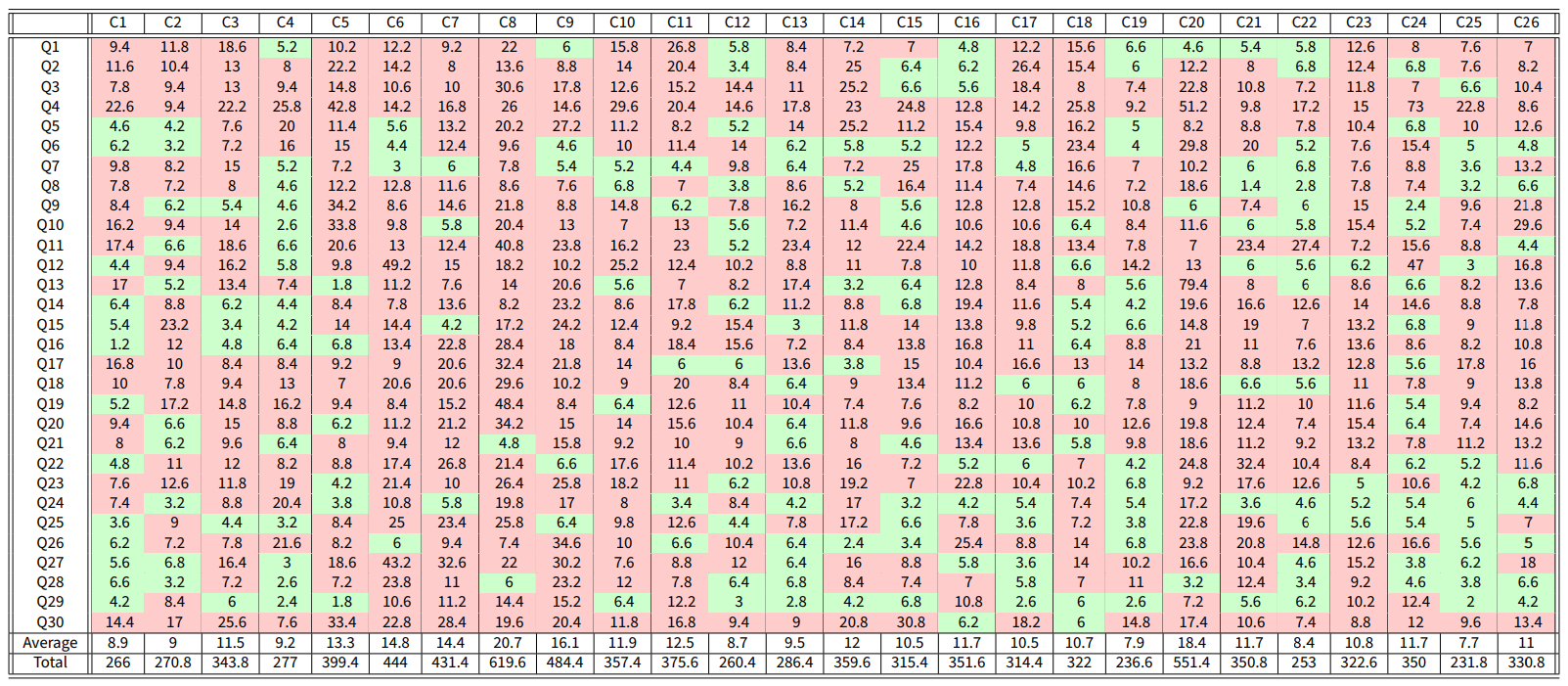
Assuming that the agents can have different inner traits for each question, Equation 11 was used to find model parameters for each country that yield opinions similar to the real ones. Once the parameters that solve the minimisation problem 11 were found for each country, the cost associated with the prediction discrepancy for each question-country pair was computed as in Equation 16 (see Figure 17) and is shown in Table 1. Due to its complexity and the huge size of the feasibility set, the minimisation problem is solved approximately: hence, a possibly suboptimal solution is found. By solving the optimisation problem more accurately, over a longer computation time (which we could not afford, due to the very large number of question-country pairs that we consider), even smaller costs could be achieved, and hence even better fits of the real data.

**Figure 17.** Visualisation of the procedure generating each column in Table 1 and of the minimisation problem in Equation 11. Assume that a survey conducted in two separate occasions in country A had $Q$ questions. Given a signed digraph $W$ and $Q$ inner traits assignations $(\psi^{(l)})_{l=1}^Q$ for each question, the model predicts a final opinion $\tilde{y}_l$, for each question. The cost function $J(y_l,\tilde{y}_l)$ measures how close the predicted final opinion is to the real final opinion $y_l$. The sum of all these costs gives the total cost $T$. Minimising the value of $T$ over the signed digraph $W$ and inner traits assignations $(\psi^{(l)})_{l=1}^Q$ gives the parameters that best reproduce the society, $\widehat{W}$, and $(\widehat{\psi^{(l)}})_{l=1}^Q$. The cost for each question and the average and total cost obtained using these optimal parameters are reported in the column of Table 1 corresponding to the considered country. All simulations evolved 100 agents.

**Table 1.** Results of the Free optimisation problem using the Classification-based model. Each column corresponds to a different country and each row to a different question. The cell values correspond to the optimal cost for all the countries and questions. The average cost along all the countries is 3.2815. The two final rows shows the column average and total. Cells with cost less than 7 are in green, the others are in red. Of the 780 possible question-country pairs, 755 have a cost less than 7 (an accuracy of $97\%$ in total). The average cost of accurate (green) question-country pairs is 2.97.

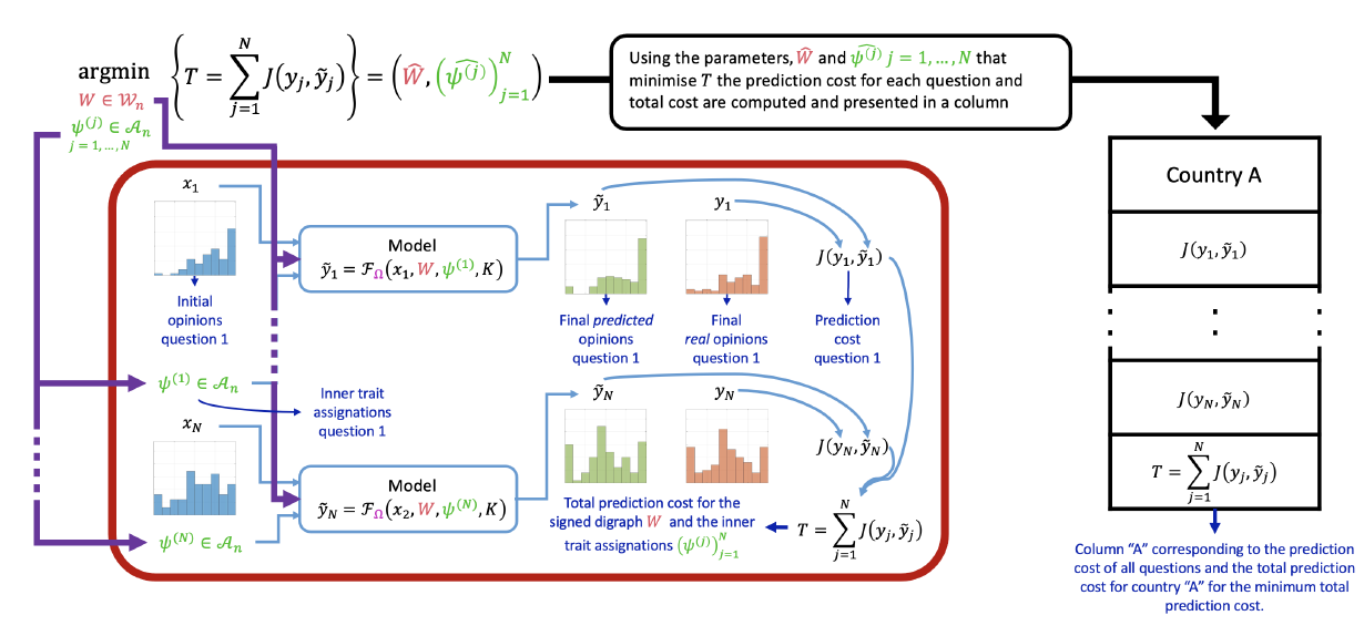
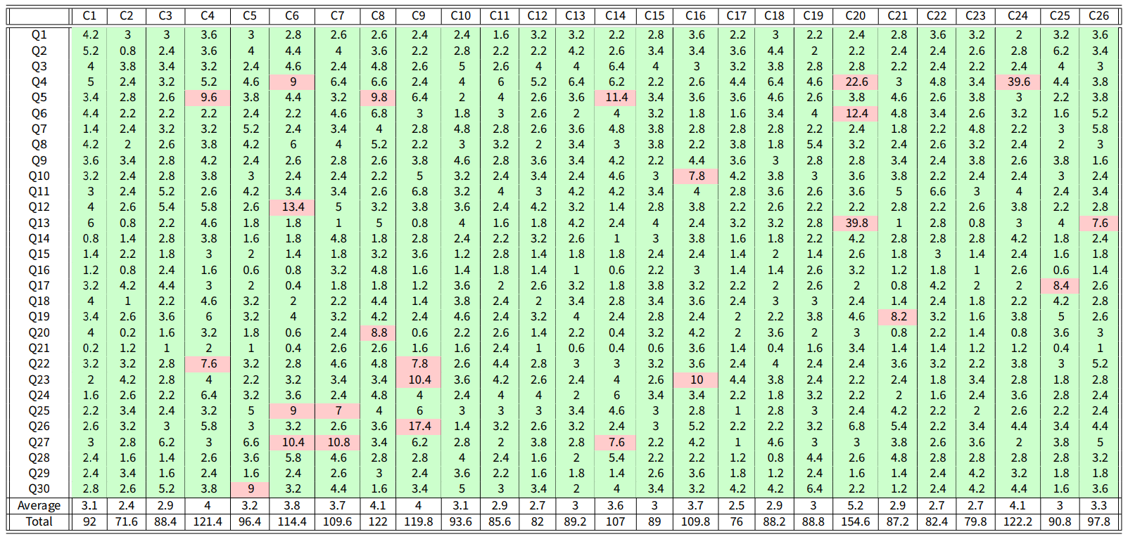
Figure 18 shows the model predictions for some question-country pairs. The original opinion is shown in blue, the real final opinion in orange, and the predicted final opinion in green; the corresponding cost $J$ (discrepancy) is reported. For costs less than 7, the model produces predicted final opinions that accurately represent the real final opinions. These cases correspond to green cells in Table 1, while cells with a cost higher than or equal to 7 are highlighted in red and constitute a small minority.

**Figure 18.** Examples of the opinion predictions achieved with the CB model, with varying resulting costs. For each trio of histograms, the initial opinions are in blue, the real final opinions in orange, and the predicted final opinions in green. The value of the cost $J$ (in Equation 16) is shown in the predicted histogram: cost values within 7 are shown to correspond to an accurate reproduction of the real opinion distribution.

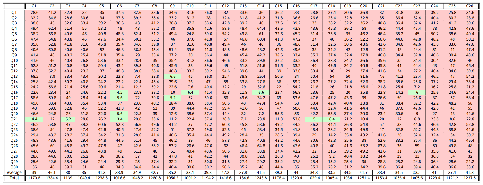
To carry out a thorough comparison with other opinion formation models, an analysis equivalent to the one reported in Table 1 is performed also for the Null (where the opinions do not change over time), the French-DeGroot (FG) (DeGroot 1974) and the Friedkin-Johnsen (FJ) (Friedkin 1986; Friedkin & Johnsen 1999) models. The results for the Null model are reported in Table 2; those for the FG model are analysed in Table 8 in Appendix A, and those for the FJ model in Appendix B. Comparing Table 1 with Table 2 shows that the CB model performs remarkably well, yielding a 97% accuracy in contrast to the 43% accuracy of the Null model: although there is a strong tendency towards stubbornness and opinion distributions tend to change only slightly over time, keeping the opinions exactly constant does not lead to good predictions.

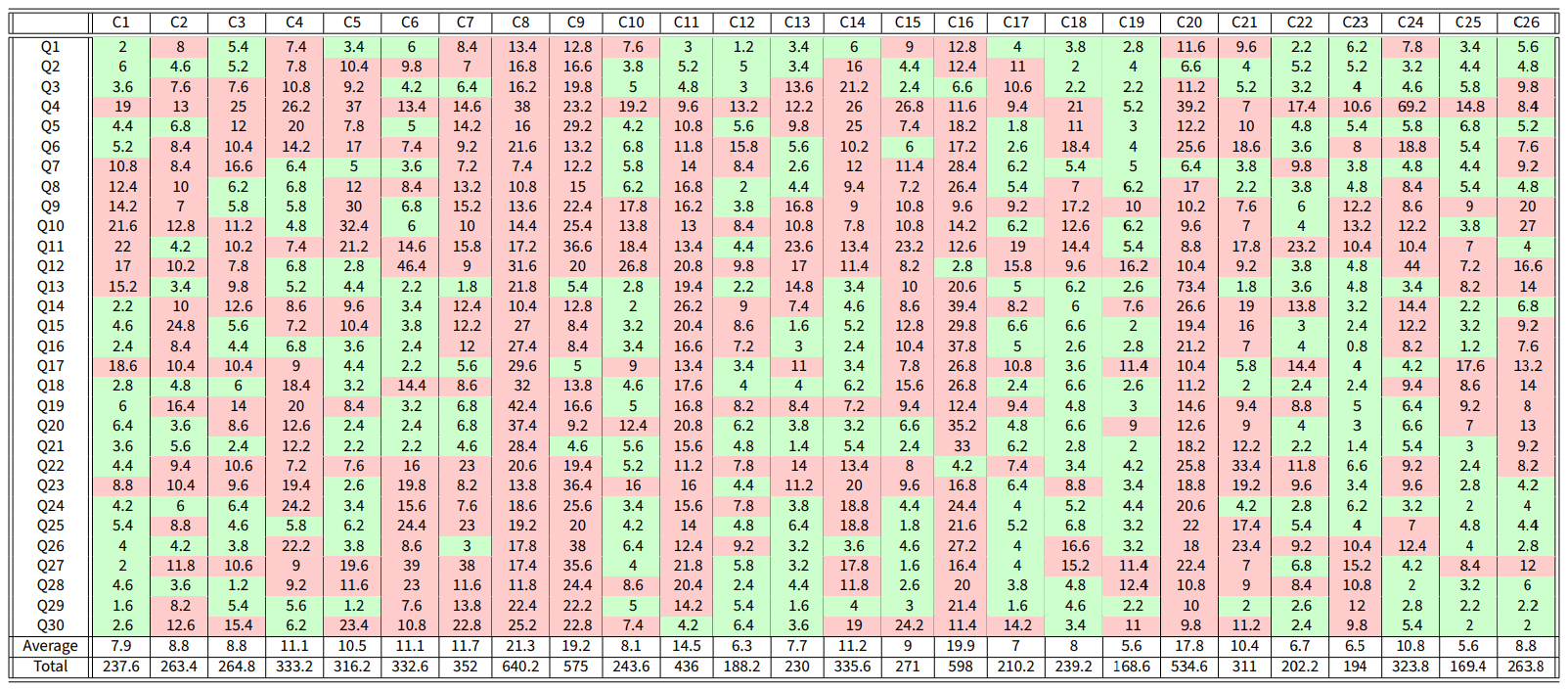
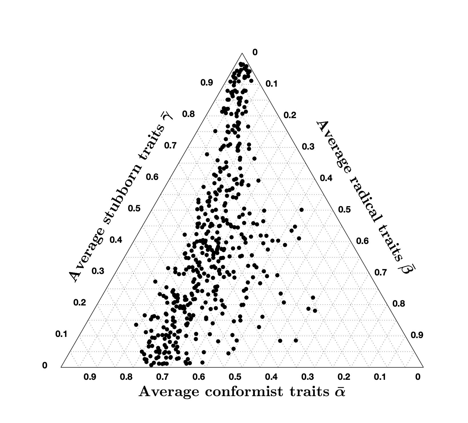
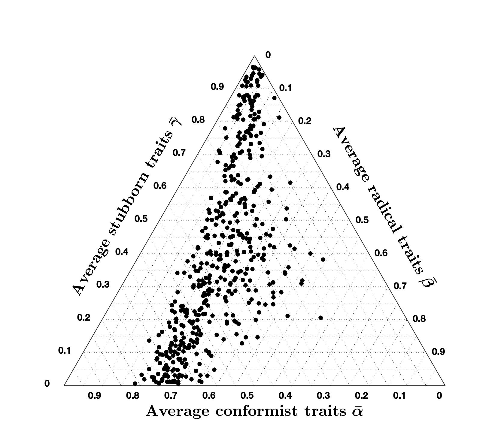
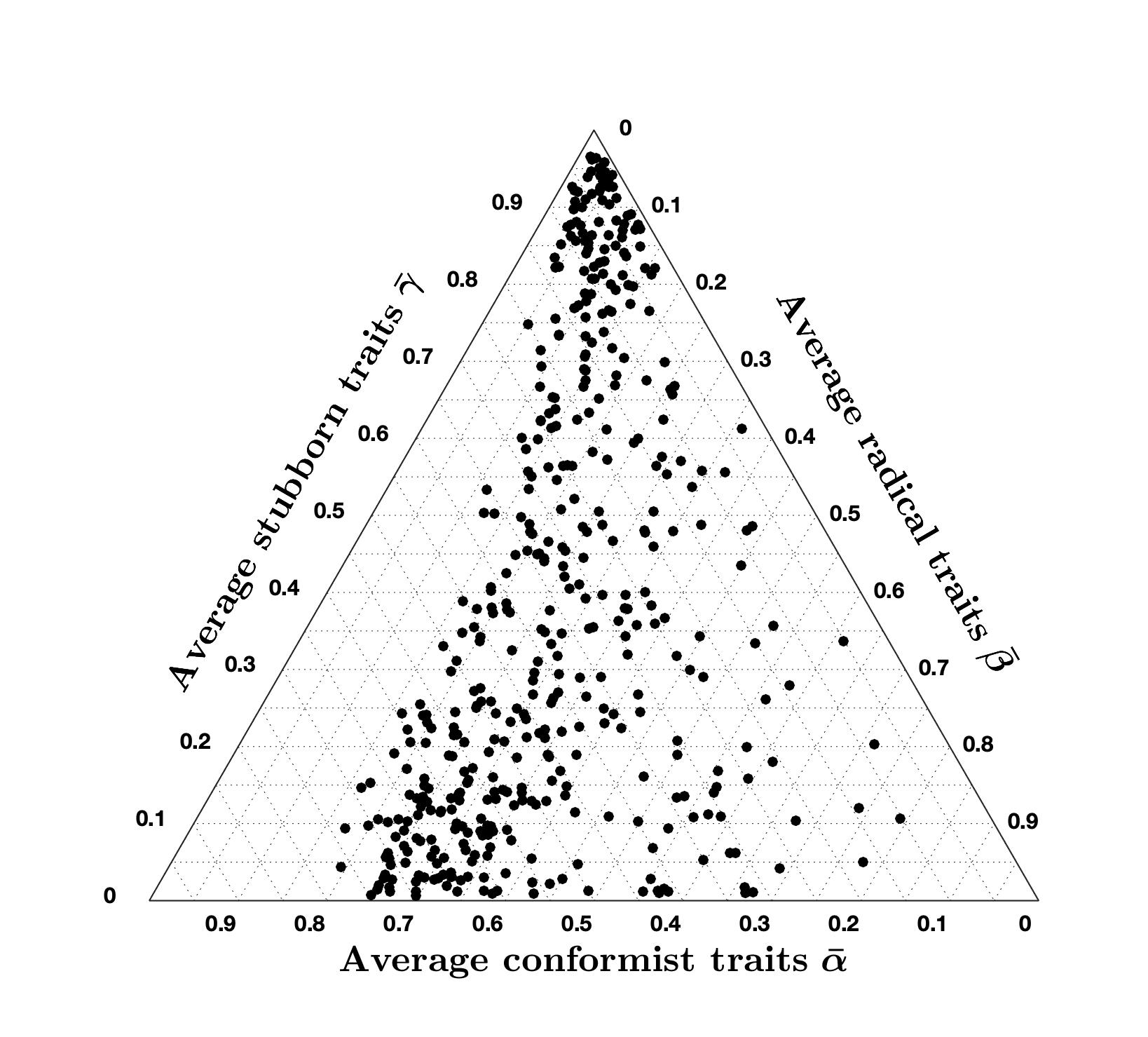
**Table 2.** Results using the Null model, for comparison with Table 1. Out of 780 possible question-country pairs, 332 have a cost less than 7 (an accuracy of $43\%$ in total). The average cost of accurate (green) question-country pairs is 4.17.

Plotting the average inner traits $\bar{\psi}$ for all question-country pairs for which the cost is less than 7 provides possible hints on how these societies could potentially be formed. However, because of the large parameter space and relatively small data set, we cannot make conclusive statements on actual societies just based on the optimisation results, as very different inner traits assignations may produce similarly low costs: we just propose a possible explanation. The resulting ternary diagram is presented in Figure 19. Figure 19a shows the position of each question-country pair. Figure 19b shows a density plot over the ternary diagram indicating the regions where most question-country pairs are found.

**Figure 19.** Analysis of the location of the average agents for all the question-country pairs with cost less than 7.

Despite the small data set and possible multiple local minima with similar low cost, fitting real data to gain an insight into the composition of actual societies reveals a clear trend: most average inner traits include a strong stubborn component, as shown by the high density in the stubbornness corner in Figure 19b. Also, the non-stubborn part can be roughly divided into $70\%$ conformist and $30\%$ radical, as shown by the trend in Figure 19a. This distribution is almost constant across all question-country pairs. Again, this is a possible explanation, and more data and more thorough explorations of the parameter space (extremely challenging from a computational standpoint) would be needed to make more conclusive statements. Hence, this is not conclusive evidence that most people are stubborn. There may be other explanations, for instance that not too many opinion exchange events take place in an average person’s life. Graph-theoretically speaking, isolation due to the lack of outgoing edges from a node (i.e., lack of interactions) is associated with the concept of stubbornness. However, from a mathematical model it is impossible to draw conclusions on whether the opinion of an agent remains unchanged because the agent refuses to consider the different opinions it is exposed to, or because the agent intentionally avoids exposure to different opinions, or because the agent simply lacks the opportunity to come into contact with different opinions. Furthermore, the traits themselves can be interpreted in different ways: for instance, a lower value of stubbornness can be regarded as a greater openness to change.

Opinion Evolution Parameter Variation: The results presented in Table 1 and Figures 18 and 19 are obtained by solving the minimisation problem 11 with nominal opinion evolution parameters $\lambda = 0.4$, $\xi = 2$, and $\mu = 5$. We now analyse the results of the minimisation problem when these parameters are changed. Tables 3 to 5 present how this variation affects the percentage of accurate question-country pairs (namely, those associated with a cost smaller than 7), the average cost of accurate question-country pairs, and the ternary diagram plot.

**Table 3:** Effects of varying $\lambda$ while keeping the nominal values $\xi = 2$, and $\mu=5$.
	$\lambda = 0.2$	$\lambda = 0.4$	$\lambda = 0.8$
% of accurate country-question pairs	93.7	96.8	97.8
Average cost of accurate country-question pairs	2.79	2.97	3.02
Ternary Diagram Plot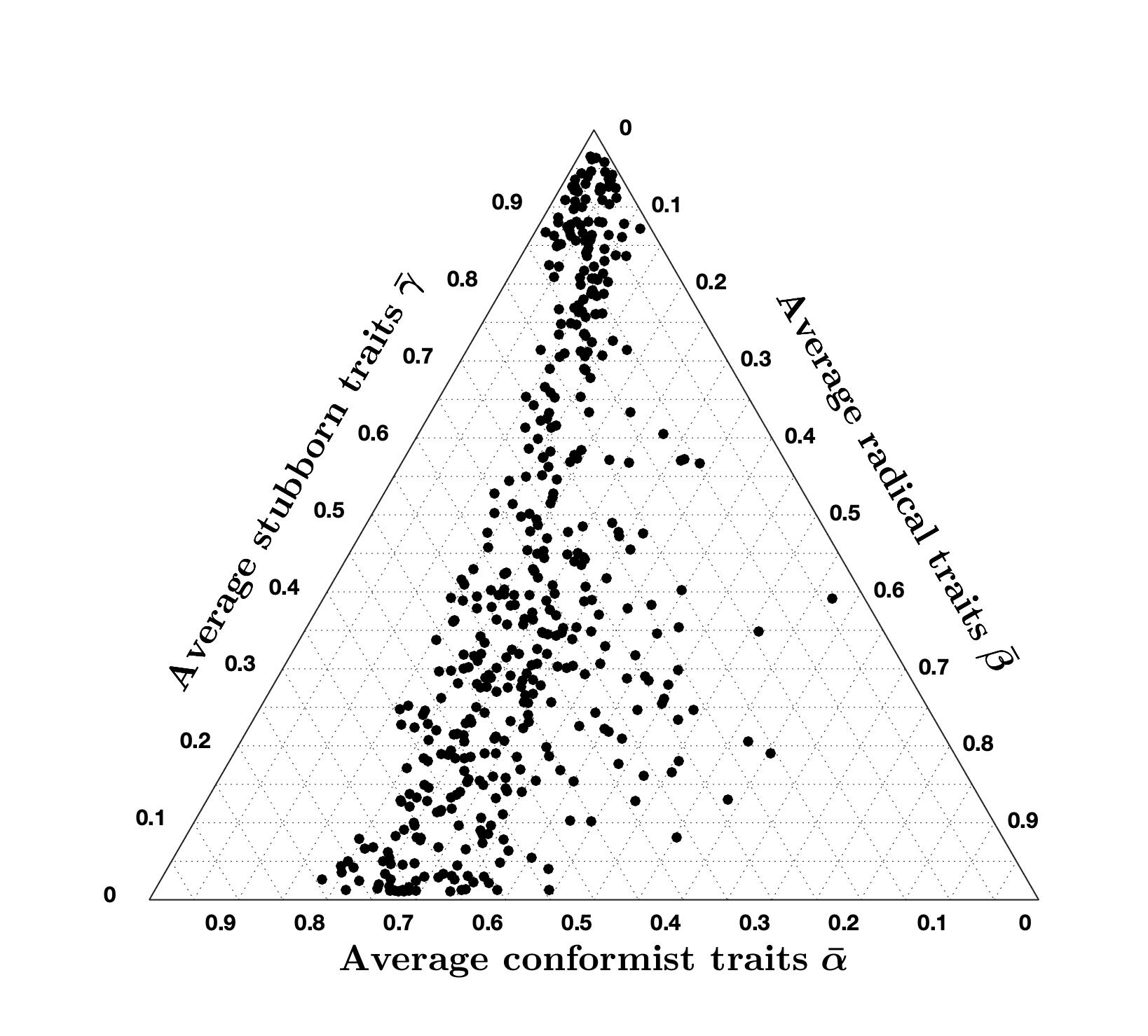

**Table 4:** Effects of varying $\xi$ while keeping the nominal values $\mu = 5$, and $\lambda=0.4$.
	$\xi = 1$	$\xi = 2$	$\xi = 4$
% of accurate country-question pairs	96	96.8	95.8
Average cost of accurate country-question pairs	2.84	2.97	3.45
Ternary Diagram Plot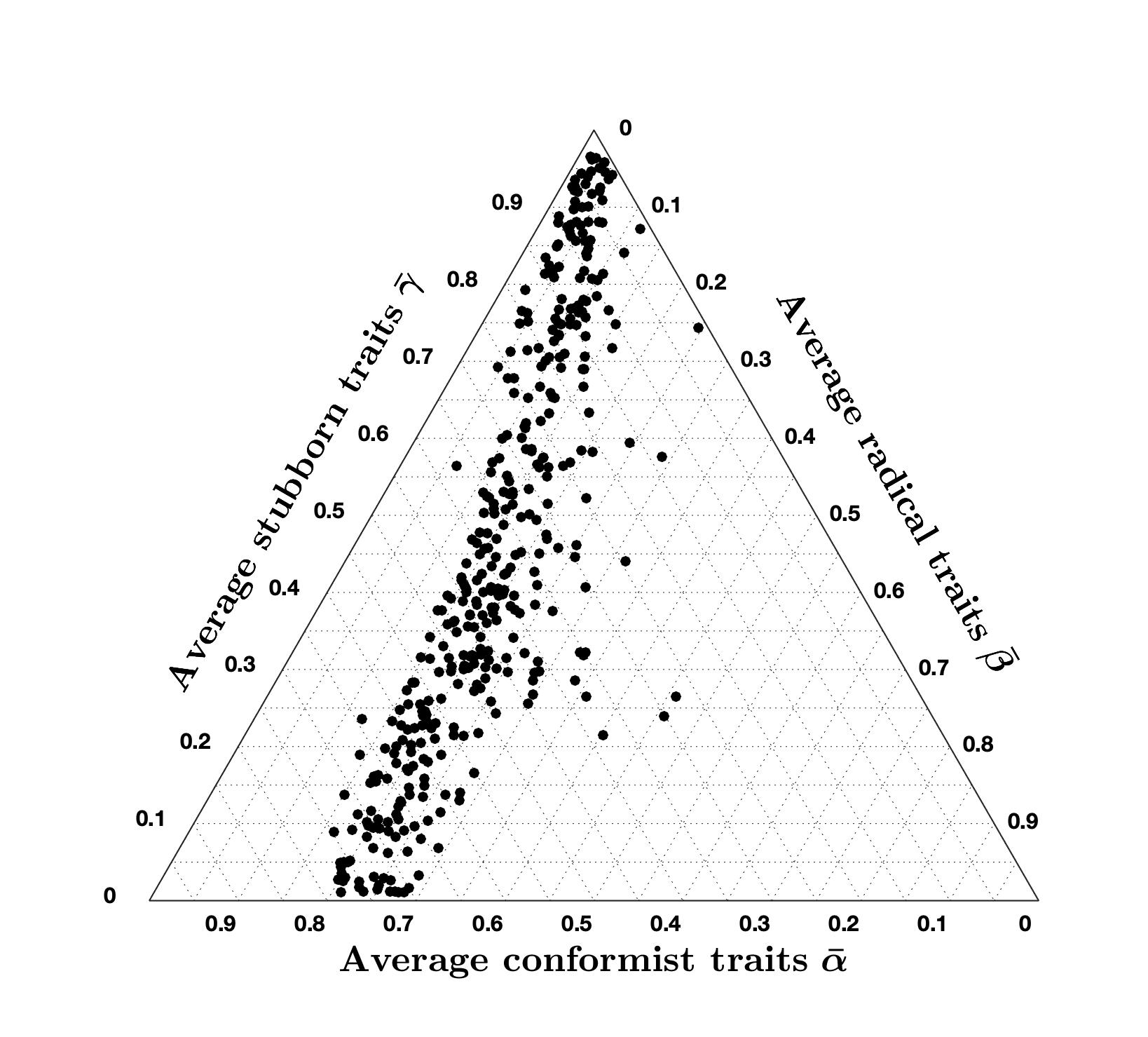

**Table 5:** Effects of varying $\mu$ while keeping the nominal values $\lambda = 0.4$, and $\xi=2$.
	$\mu = 2.5$	$\mu = 5$	$\mu = 10$
% of accurate country-question pairs	96.8	96.8	97.2
Average cost of accurate country-question pairs	2.84	2.97	3.15
Ternary Diagram Plot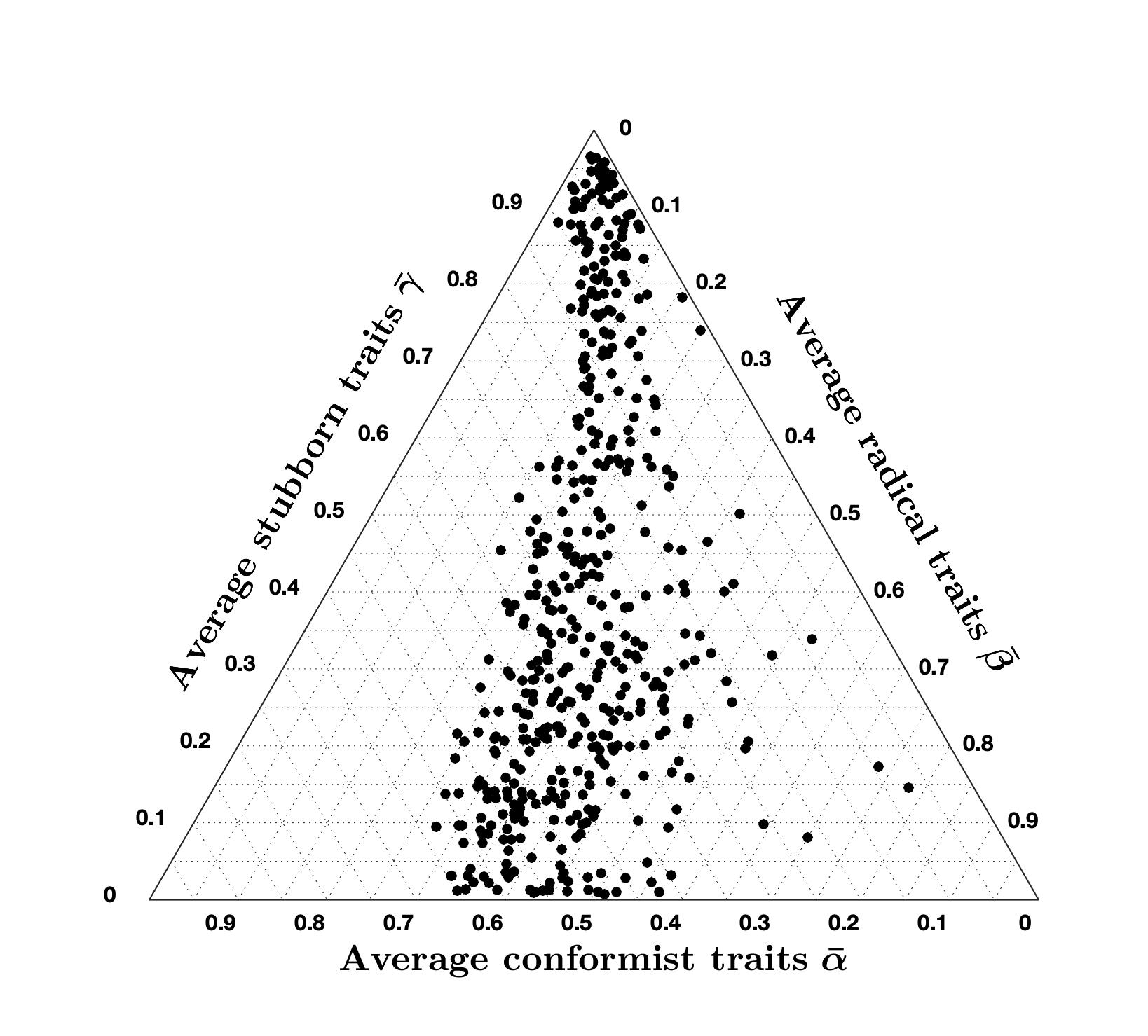

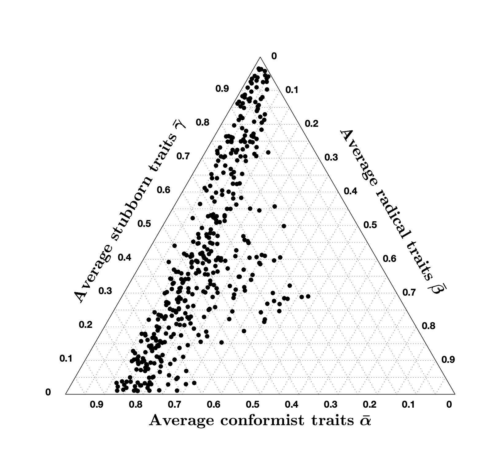Tables 3 to 5 show that, even after varying the values of $\lambda$, $\xi$, and $\mu$, the percentage of accurate question-country pairs remains around $96\%$, and the average cost of accurate question-country pairs is between $2.79$ and $3.45$ which is quite remarkable since it means that the high accuracy achieved with the CB model is very robust to variations in the opinion evolution parameters $\lambda$, $\xi$, and $\mu$ (while it is not robust with respect to changes in signed digraph weights or inner trait assignations, see Figure 2).

Comparing the ternary diagrams shows the persistent tendency of question-country pairs to lie along a line where the proportion between conformist and radical traits is constant. For most simulation results, this proportion is still $70\%$ conformist and $30\%$ radical, as in the nominal case (Figure 19a). The proportion only changes when varying $\mu$: for $\mu = 2.5$, we have $60\%$ conformist and $40\%$ radical agents, while for $\mu = 10$ we have $80\%$ conformist and $20\%$ radical agents. Therefore, it appears that $\mu$ can be tuned to regulate this proportion.

Constrained optimisation problem

If the agents are assumed to have the same inner traits for every question, then the model parameters can be found using the constrained optimisation problem in Equation 12. One advantage of using this approach is that, since each country has the same topology and inner traits assignation for all the questions, these parameters can be identified by solving the constrained optimisation problem 12 for a subset of all available questions (training dataset), and then tested on the remaining questions (test dataset). This was not possible previously, when assuming a different inner traits assignation associated with each question.

This procedure is commonly known as cross-validation. Generally, a subset of available data is used to train an algorithm (in this case, to identify the model parameters $\widehat{W}$ and $\widehat{\psi}$) and the remaining data is used to test the trained algorithm (in this case, the model with identified parameters $\widehat{W}$ and $\widehat{\psi}$). To eliminate result biases due to the selected training datasets and test datasets, cross-validation is performed multiple times for different partitions of the data. A common approach is to divide the data in $K$ subsets and validate the model $K$ times so that, at each iteration, only one subset is taken as the test dataset. This is known as $K$-fold cross-validation.

Table 6 shows the result of sixfold cross-validation on the available data (the questions are divided in six subsets of five questions each: $\{1, \dots, 5\}$, $\{6, \dots, 10\}$, $\dots$, $\{26, \dots, 30\}$ ). The first six rows show the mean cost for the five questions in the test dataset for each country for each cross-validation (CV1 to CV6). The last row shows the mean of the first six rows.
The simulation results summarised in Table 6 show that the model is able to accurately reproduce the final opinions for the tested data. Although the values are higher than 7, it is important to note that these predictions are done based on the assumption that the inner traits are the same for every question, while in reality the inner traits of the agents may change when considering their attitude towards different types of questions (which is taken into account by the free optimisation approach).

**Table 6.** Results of the sixfold cross validation. Each column corresponds to a country, and each row to one of the six cross validations. The value in cell $(i,j)$ is the average cost of the test data in cross validation $i$ for country $j$. The last row represents the mean over all the rows.

Table 7 is analogous to Table 1, but now the model parameters are obtained with the Constrained optimisation problem 12, which yields a higher cost, as expected, since the optimised inner traits assignations can be very different when unconstrained, see Figure 19a.

**Table 7.** Results of the Constrained optimisation problem using the Classification-based model. The average cost along all the countries is 11.6746. Out of 780 possible question-country pairs, 220 have a cost less than 7 (an accuracy of $28\%$ in total). The average cost of accurate (green) question-country pairs is 5.16.

Summary and Conclusions

We have proposed a novel agent-based opinion formation model that has two fundamental distinctive features. First, the model drops the unrealistic assumption that agents can measure the opinion of their neighbours with infinite precision, which drastically affects the opinion evolution, and introduces a novel classification-based approach that more realistically replicates the way individuals assess and evaluate the opinions of their neighbours, by classifying them as agreeing much less, less, comparably, more or much more. Second, the model captures the complexity of the behaviour of individuals by introducing three different internal traits, associated with conformism, radicalism, and stubbornness. Instead of considering agents of different types, the model allows all these tendencies to coexist in each agent, thus representing multifaceted psychological and sociological phenomena in action within each individual.

In addition to the agent parameters and the underlying digraph, the model simply relies on three parameters, $\lambda$, $\xi$, and $\mu$, having a natural interpretation. Based on a deterministic classification mechanism, the opinions evolve over discrete time steps according to the deterministic Equation 7. The signed underlying digraph is time-invariant. Despite its simplicity, the model can recreate opinion evolutions seen in real-life and produce a rich and wide variety of collective behaviours, without the need of introducing bounded confidence, randomness, or more complex mechanics.

Four types of simulation analyses were carried out: ($i$) simulations over simple digraph and agent parameters to gain insight into the model behaviour; ($ii$) simulations with varying model parameters to perform a parameter sensitivity analysis; ($iii$) model outcome capabilities, studied using distributional measures such as the recently proposed Bias, Diversity, and Fragmentation (Lorenz et al. 2021); ($iv$) simulations with parameters chosen through the approximate solution of two optimisation problems to assess the model’s potential to recreate opinions similar to those seen in real life.

We used real data from the World Values Survey to assess the capability of our Classification-based model to mimic actual opinion evolutions seen in real life: building a link between theoretical opinion dynamics modelling and empirical data in social research is a strong focus of this work.

Our results can be relevant in future research on opinion formation models in several ways. The proposed CB model offers a flexible general framework that can be easily adapted to combine other psychological traits, change the mathematical formulation of the current traits, or include agents with more accurate opinion perception (by increasing the number of sets an agent can classify its neighbours in); additional analyses can be performed to assess how these variations would affect the model behaviour and characteristics.

The link between survey results and model outcomes, with parameters chosen via suitable optimisation problems, is also of value to future research on opinion formation models: the field has great potential to grow by systematically connecting empirical and theoretical findings. Our proposed methodology can be tailored to the available data and the focus of the study: possible changes include embedding constraints that correlate the agent opinions, their parameters, and their location in the network, and a combination of the ‘free’ and ‘constrained’ problems.

Our analyses and simulations have highlighted the model properties and behaviour, thus answering the following questions.

What does the model actually do? Quantitatively, the model evolves by iterating Equation 7. Qualitatively, the combination of the classification mechanism and psychological traits results in agents having two main behaviours: mostly conformist agents aim for consensus with their neighbours, while mostly radical agents move toward extreme opinions. The stubborn trait slows the opinion evolution, without affecting its trend. The collective population dynamics is a combination of these effects, which makes the model particularly flexible and enables a wide range of opinion outcomes: the model can generate opinion distributions ranging from extreme polarisation to consensus, depending on the agent parameters. Due to the imperfect opinion perception, the agents rarely converge to the exact same non-extreme opinion, even if they all are completely conformist.
What does the model teach us about human behaviour? The model provides some interesting indications. The ability of the Classification-based model to recreate opinion transitions seen in real populations suggests that radicalism is an essential trait in the opinion formation mechanism, when modelling large-scale opinion evolution. Additionally, the model also shows that radicalism alone does not necessarily lead to polarisation: polarisation only occurs when the population is mostly radical and the initial opinions are mostly divided (comparably the same number of agents agree and disagree).
What kind of dynamics does the model produce and why does it produce these dynamics? Since the stubbornness trait mainly slows the opinion evolution, let us focus on the other two traits. Completely conformist societies move towards the mean of the initial opinions (without reaching consensus on a single opinion, but asymptotically driving all opinions in the neighbourhood of a given opinion). As radicalism increases, some agents move to extreme opinions and influence other agents, resulting in a more diverse or partitioned set of opinions (possibly forming clusters). If radicalism keeps increasing, at some point all the agents move to extreme opinions, resulting in either polarisation, or consensus at either complete agreement or complete disagreement. The sign of the edges of the signed digraph has a more subtle effect. Increasing the fraction of negative edges makes the dynamics less obvious to predict, especially when most agents are conformist: if the digraph is sufficiently unbalanced, the opinions move towards $0$ (as it happens with a structurally unbalanced network in the model by Altafini (2013)); if the signs are suitably arranged, opinions may also converge to values that are not near the initial opinion mean.
Are any of the results surprising in some way? The significant effect of radicalism on the opinion evolution in a large population is remarkable. The model shows that radicalism is more impactful than conformism (see for instance the simulations with only radical and conformist traits in Figure 4); this effect may be due to the mathematical implementation of the radical trait. It is also surprising that the sign of the digraph edges has such a subtle effect, while for instance in the Altafini model its impact on the opinion evolution is much more noticeable.

A particularly interesting direction for future work is the formulation and solution of the optimisation problems that include correlation constraints between initial opinions, agent parameters, and location in the network. An optimisation problem that is located between the ‘constrained’ and ‘free’ problems would also be interesting to define: the agent parameters for each question may be allowed to be different, but within a maximum possible difference, to represent the case in which the agent traits can change depending on the question, but cannot be completely different because each agent preserves some main personality traits across questions. This ‘hybrid’ optimisation problem could then be solved using heuristic approaches, such as genetic algorithms. This could be a possible way to advance in the solution of the inverse problem for opinion formation models, and as such would be a considerable progress in the direction of studying opinion dynamics with empirical data. Additional research directions are to study of the effects on the opinion evolution of different network topologies, opinion-dependent agent parameters, and the effect of opinion evolution parameters $\Omega$ that are agent-dependent.

Appendix A: Comparison with the French-DeGroot model

Here, an optimisation problem analogous to the Constrained optimisation problem for our CB model is solved for the classical French-DeGroot (FG) model. It is important to note that the two models aim at reproducing opinion evolution dynamics in completely different contexts: the FG model was developed for small-group interactions over a relatively short time interval, usually leading to consensus; the CB model aims to recreate opinion changes in large-scale societies over long time intervals, as indicated by the use of country-wide survey results with approximately 5 year separation. Still, it is interesting to see how the results differ.

To make Tables 1 and 8 comparable, for the FG model the digraphs used in each country are selected following the same minimisation problem as the one solved for the CB model. Since the FG model does not involve agent parameters, we only minimise over the set of digraphs $\mathcal{W}_\text{FG}$. Both the set of digraphs for the CB model, $\mathcal{W}$, and for the FG model, $\mathcal{W}_\text{FG}$, have the same number of elements and there is a one-to-one topology correspondence; the digraphs in $\mathcal{W}$ are signed and unweighted, while those in $\mathcal{W}_\text{FG}$ are unsigned and row-stochastic (as required by the different nature of the two models). As expected, the FG model, focused on small-group consensus processes, does not lead to accurate predictions of opinion changes in large societies for long time intervals.

**Table 8.** Results of the optimisation problem using the French-DeGroot model, for comparison with Table 1. The average cost along all the countries is 38.4323. Of the 780 possible question-country pairs, 13 have a cost less than 7 (an accuracy of $2\%$ in total). The average cost of accurate (green) question-country pairs is 5.43.

Appendix B: Comparison with the Friedkin-Johnsen Model

The Classification-based model can be seen as an extension of the Friedkin-Johnsen (FJ) model (Friedkin 1986; Friedkin & Johnsen 1999), in the sense that both models include in the agents’ behaviour inner traits described by tuples. In the FJ model, each agent $i$ is characterised by two parameters: susceptibility $a_i\in[0,1]$, determining how strongly the agent is affected by its neighbours’ opinions and forgets the initial opinion (Friedkin & Johnsen 1999), and prejudice $b_i = 1-a_i\in[0,1]$. A value of $a_i = 1$ means that the agent has complete susceptibility to interpersonal influence (similar to complete conformism), while a value of $a_i=0$ means that the opinion remains the same for all times (similar to complete stubbornness). In the CB model, each agent $i$ is associated with three parameters: conformism $\alpha_i\in[0,1]$, radicalism $\beta_i\in[0,1]$, and stubbornness $\gamma_i\in[0,1]$, such that $\alpha_i+\beta_i+\gamma_i = 1$ for all $i\in V$. Therefore, a FJ model where all agents have a susceptibility of $a$ is similar to a CB model where all agents have inner traits $\alpha = a$ and $\gamma = 1-a$ (hence $\beta=0$). Still, the interpretations of stubbornness and prejudice are slightly different: prejudice in the FJ model means that agents tend to keep their initial opinion, while stubbornness in the CB model means that agents tend to keep their current opinion, which leads to the same outcome only when all the agents are completely stubborn. Apart from the outlined similarity, the FJ and CB models are different: crucially, the FJ model is linear, while the CB model is highly non-linear, which severely limits the applicability of closed-form analysis tools.

Figure 20 shows the evolution of the same initial opinions according to the two models, for different values of $a$, $\alpha$, and $\gamma$. The digraphs have the same topology; randomly generated weights are considered for the FJ model, while for the CB model all the edge signs are taken positive to match the absence of antagonism in the FJ model. The FJ model exhibits a slower change as $a$ increases, while with the CB model, as soon as conformism is introduced, the opinions converge to an interval where all the agents perceive that their neighbours’ opinion is similar enough to theirs. This difference is caused by the two different interpretations and implementations of stubbornness and prejudice. Another important difference is that, as the susceptibility value increases, the final opinions of the FJ model tend to converge to a single opinion, and yield perfect consensus when $a=1$. Conversely, the final opinions of the CB model never converge to perfect consensus, even when $\alpha=1$ and $\gamma=0$, as a consequence of the classification-based approach.

**Figure 20.** Comparison between the Friedkin-Johnsen (FJ) model, for different values of susceptibility $a$, and the Classification-based (CB) model, for corresponding values of conformist ($\alpha$) and stubborn ($\gamma$) weights. All the 100 agents have the same values of $a$ (FJ) and of $\alpha$ and $\gamma$ (CB). The simulations start from the same initial opinions and evolve over digraphs with the same topology. The degree of susceptibility, prejudice, conformism, and stubbornness is represented by the colours cyan, magenta, blue, and green respectively.

The differences between CB and FJ model help visualise the strong implications of the classification-based mechanism for assessing the opinion of others, which captures the fact that opinions cannot be perceived with perfect resolution and accuracy, and hence changes the model behaviour significantly: it grants the model new properties, such as the existence of multiple equilibria that can span the complete spectrum of opinions. For instance, in Figure 20, the CB model with $\alpha = 1$ and $\gamma = 0$ generates equilibrium opinions that span almost $40\%$ of the opinion interval $[-1,1]$ (a wider span can be achieved with different topologies), while the FJ model with $a = 1$ leads to identical equilibrium opinions. The non-linearity introduced by the classification-based assessment of the opinion of others can completely change the resulting dynamics and lead to the emergence of peculiar features, which would not emerge from models where the agents have perfect access to the opinion of others, as the comparison with the Friedkin-Johnsen model highlights.

The results of an analysis for the FJ model, equivalent to the one reported in Tables 1 and 7 for the CB model, are reported in Tables 9 and 10. To make the results comparable, when solving the optimisation problems 11 and 12 for the FJ model the sets $\tilde{\mathcal{A}}$ and $\tilde{\mathcal{W}}$ are modified as follows: the topology of each network in the set $\tilde{\mathcal{W}}$ is kept the same, but the weights are changed so that they are all positive and the associated adjacency matrix is row-stochastic. The inner traits assignations in $\tilde{\mathcal{A}}$ are transformed into parameters of the FJ model using the mapping $a_i = \alpha_i/(\alpha_i + \gamma_i)$; if $\alpha_i + \gamma_i = 0$, then $a_i = 0.5$.

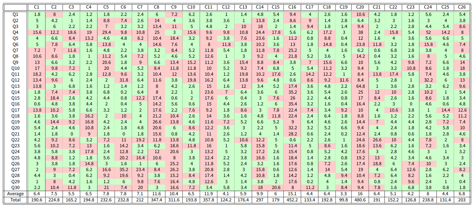
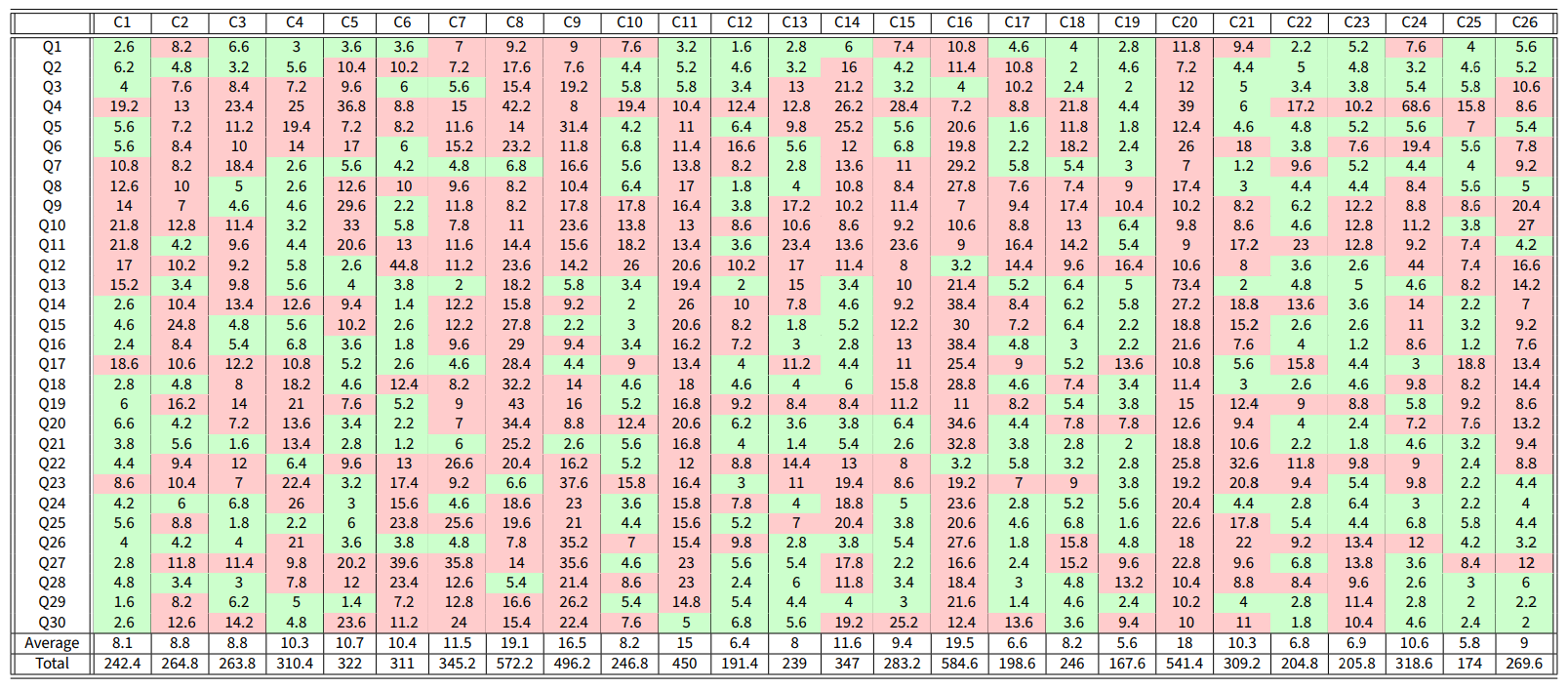
**Table 9.** Results of the Free optimisation problem using the Friedkin-Johnsen model. The average cost along all the countries is 7.4897. Out of 780 possible question-country pairs, 460 have a cost less than 7 (an accuracy of $59\%$ in total). The average cost of accurate (green) question-country pairs is 3.3.

**Table 10.** Results of the Constrained optimisation problem using the Friedkin-Johnsen model. The average cost along all the countries is 10.3918. Out of 780 possible question-country pairs, 330 have a cost less than 7 (an accuracy of $42\%$ in total). The average cost of accurate (green) question-country pairs is 4.1.

Comparing Tables 1 and 9 shows that the CB model outperforms the FJ model, yielding a 97% accuracy in contrast to 59%. Also, the average cost of country-question pairs with cost less than 7 is lower for the CB model (2.97) compared with the one produced by the FJ model (3.3), indicating that not only more question-country pairs are predicted satisfactorily, but also the predictions are more accurate.

General agreement analysis

Given a single initial opinion vector $x_o$ and a set of inner traits assignations $\mathscr{A}$ and networks $\mathscr{N}$, let $X = X(x_o, \mathscr{A}, \mathscr{N})$ be the set of all final opinion vectors produced by evolving the initial opinions $x_o$ with inner traits assignation $\psi\in\mathscr{A}$ over a network $W\in\mathscr{N}$. The plot of the general agreement $(\theta_+, \theta_-)$, as defined in Equation 14, of each final opinion vector in $X(x_o, \mathscr{A}, \mathscr{N})$ in the Cartesian plane gives a visual representation of the range of opinions that the model can produce starting from $x_o$. Figure 21 shows this plot for five different initial opinion vectors (seen in Figure 22) for the CB and the FJ models. In the plots, each dot is colour-coded: for the CB model, the colour represents the average inner traits (blue for average conformist trait $\overline{\alpha}$, red for average radical trait $\overline{\beta}$, and green for average stubborn trait $\overline{\gamma}$); for the FJ model, it represents the average susceptibility $\overline{a}$ (cyan represents complete susceptibility $\overline{a} = 1$ and magenta complete prejudice $\overline{a} = 0$). We consider the same set of traits as for the optimisation problem, i.e., $\mathscr{A}=\tilde{\mathcal{A}}$, and a set of networks $\mathscr{N}$ including networks 1 to 5 in $\tilde{W}$, selected because they represent networks with the same topology and varying ratio of negative to positive edges.

**Figure 21.** Row 1 (respectively, row 2) shows the general agreement plot of the potential opinion vectors predicted by the FJ (respectively, CB) model, starting from the initial opinion vectors shown in Figure 22. The marker colour encodes the average traits of the agents producing the final opinion: for the FJ model, cyan and magenta represent susceptibility and prejudice respectively; for the CB model, blue, red and green represent conformism, radicalism and stubbornness respectively. All simulations evolved over 50 time steps.

**Figure 22.** Initial conditions for the opinion evolutions shown in Figure 21

Figure 21 highlights that the CB model can produce a wide range of predicted opinions, primarily thanks to the interaction of the three complementary inner traits: conformism brings opinions together, yielding an effect that is similar to that of the FJ model, i.e., moving opinions along the $3\pi/4$ diagonal; radicalism allows the opinions to move in the other 3 diagonal directions ($\pi/4$, $5\pi/4$ and $7\pi/4$); and stubbornness makes opinions stay near the initial opinion. The combined effect of multiple combinations of these traits leads to possible predicted opinions that have a greater range than the ones produced by the FJ model.

Susceptibility or conformism could be considered as a trait that moves all the opinions towards a common opinion in the middle of the interval $[-1,1]$, whereas radicalism moves all the opinions to their corresponding extremes, either $-1$ or $1$. The combined effect moves the opinions across the interval $[-1,1]$, and the degree of stubbornness determines the speed of the change. Interestingly, if the initial opinion is above the line $\theta_+ = -\theta_-$, then the predicted opinions also tend to stay above the line: if the overall population agrees more than it disagrees with a statement, this opinion balance is likely to be preserved, this was already noted in Figure 16. However, a change in opinion balance is not impossible: a considerable fraction of predicted opinions may approach the line $\theta_+ = -\theta_-$, and from there a change in population traits may move the predicted opinions to the other side of the line (initial opinion 2 can produce an opinion vector near initial opinion 1 and from there the next opinions can be near initial opinion 3). It is also interesting to note that, although initial opinions 1 are slightly below the $\theta_+ = -\theta_-$ line, most of the predicted opinions are above that line, an effect probably caused by the network topology or the edge signs.

Appendix C: Optimisation Approach

The subset $\tilde{\mathcal{W}}$ contains 35 different small-world signed strongly connected digraphs. Table 11 shows the values of the main metrics for the networks.

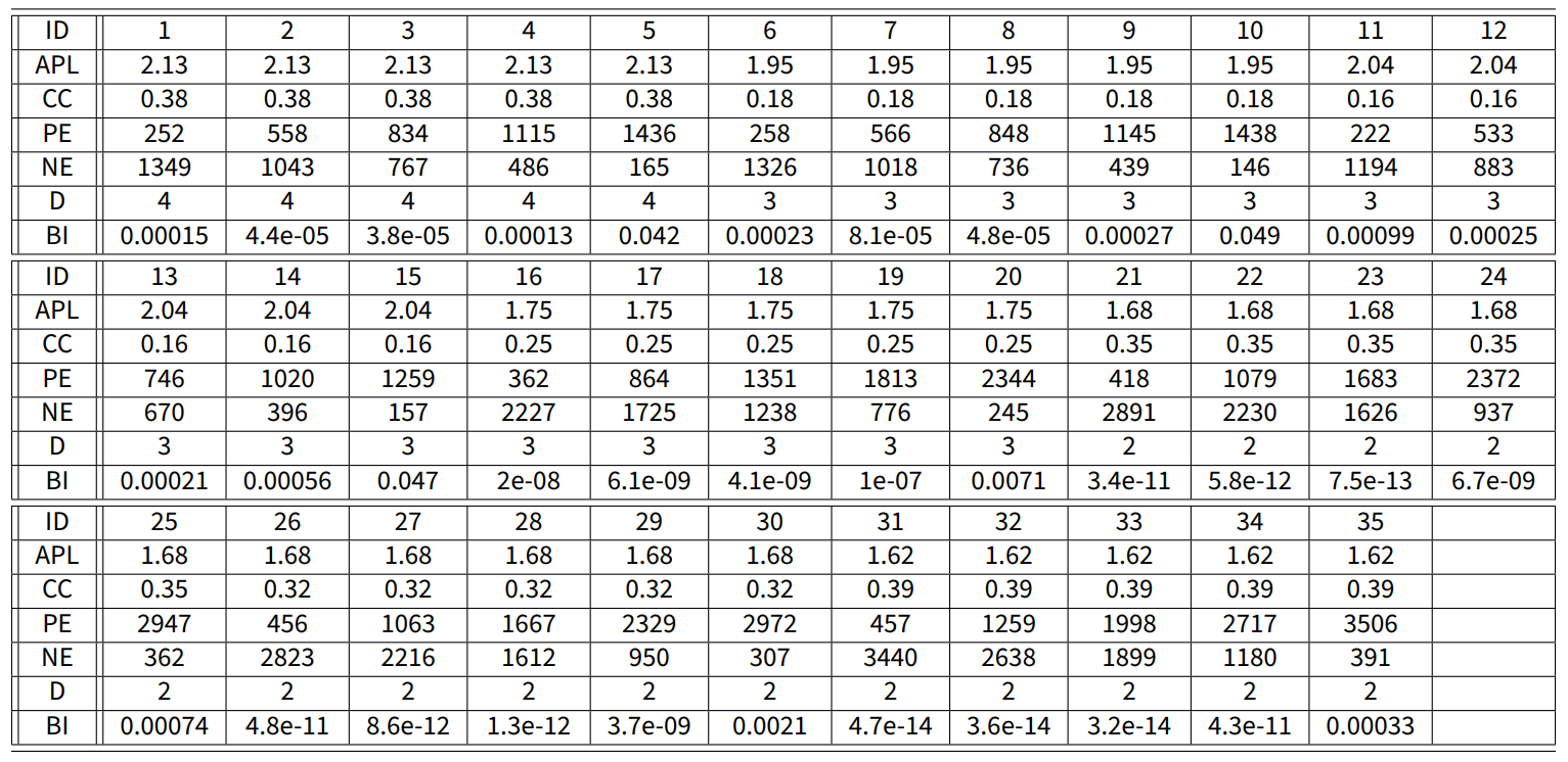
**Table 11.** Signed Digraph Information: Average Path Length (APL), Clustering Coefficent (CC), Positive Edges (PE), Negative Edges (NE), Diameter (D), and Balance Index (BI)

The subset $\tilde{\mathcal{A}}$ contains $3528$ randomly generated inner traits assignations $\psi= (\psi_i)_{i=1}^n$. To avoid bias towards societies with average inner traits that are more conformist, radical, or stubborn, the set $\tilde{\mathcal{A}}$ satisfies the following property: for every inner traits assignation $\psi$, with corresponding average inner trait $\bar{\psi} = (\bar{\alpha}, \bar{\beta}, \bar{\gamma}) = (a_1, b_1, c_1)$, there are two inner traits assignations $\psi^\prime, \psi^{\prime\prime}\in\tilde{\mathcal{A}}$ that satisfy $\bar{\psi^\prime} = (b_1, c_1, a_1)$, and $\bar{\psi^{\prime\prime}}= (c_1,a_1,b_1)$. In other words, the parameter space $\tilde{\mathcal{A}}$ is symmetric with respect to permutations of agent traits. Besides this property, the elements of this set were chosen at random. All the average inner traits $\bar{\psi}$ corresponding to inner traits assignations $\psi$ in $\tilde{\mathcal{A}}$ are shown in Figure 23.

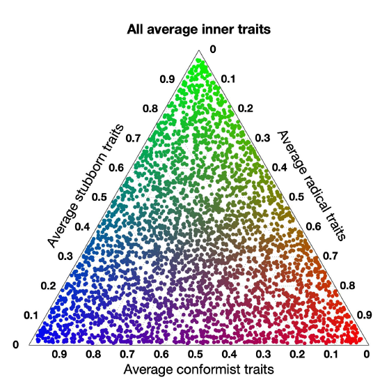
**Figure 23.** All the average inner traits $\bar{\psi}$ corresponding to inner traits assignations $\psi$ in $\tilde{\mathcal{A}}$.

Due to the anonymity of the surveys, it is not possible to guarantee that the same people answered the survey in subsequent waves of the WVS. However, if the surveys are done correctly to represent society overall, the results can be anyway assumed to reflect the global opinion distribution of the general population about a given topic at a specific time, and this allows us to use the survey results in different waves in our minimisation problem, as if the very same people had answered. Moreover, even though all our simulations could be run for an arbitrary number of agents, we consider $n=100$ agents (as representatives of the whole society) to keep the computational demand (especially for the optimisation problem) manageable.

Appendix D: Network Metrics

The signed digraph is represented by the weight matrix $W\in\{-1,0,1\}^{n\times n}$, where $w_{ij}$ is associated with the edge going from vertex $j$ to vertex $i$. We consider six network metrics: average path length (APL), clustering coefficient (CC), positive edges (PE), negative edges (NE), diameter (D), and balance index (BI). This appendix explains how these metrics are computed.

A directed path is a $K$-tuple of vertices $(p_1, p_2, \dots, p_i, p_{i+1}, \dots , p_K)$ such that there is an edge from vertex $p_i$ to vertex $p_{i+1}$ for $i=1, \dots, K-1$. The length $|p|$ of a directed path $p$ is the number of edges that it crosses. Let $P(i,j)$ be the set of all directed paths from vertex $i$ to vertex $j$ (if there are none, then $P(i,j) = \emptyset$). Denote by $d(i,j)$ the length of the shortest directed path from $i$ to $j$, i.e., $d(i,j) := \min_{p\in P(i,j)}|p|$. Let $C(W)$ be the set of vertex pairs $(i,j)$ such that there exists a direct path from $i$ to $j$ and $i \neq j$, i.e. $C(W) = \{(i,j)\mid P(i,j) \neq \emptyset \text{ and } i \neq j \}$. Then the average path length and diameter of the digraph $W$ are:

\[APL = \frac{1}{|C(W)|}\sum_{(i,j)\in C(W)}d(i,j) \qquad\mbox{and}\qquad D = \max_{(i,j)\in C(W)}d(i,j)\]

\[(18)\]

Note that, because all the networks are strongly connected, $|C(W)| = n(n-1)$.

To compute the clustering coefficient, consider agent $i$, with $k_i$ in-neighbours excluding itself: $k_i = |\tilde{\mathcal{N}_i}|$, where $\tilde{\mathcal{N}_i} := \{ j\in V\mid w_{ij}\neq0, i \neq j\}$. Then there are at most $k_i(k_i-1)$ directed edges between these neighbours. The fraction $c_i$ of these edges that is actually present is the clustering coefficient of agent $i$. If agent $i$ has only one in-neighbour, then its clustering coefficient is 1, and if it has no in-neighbour but itself $c_i$ is not defined:

\[c_i = \begin{cases} \frac{|\{ (j,k) \mid j \neq k \text{ and } i,k\in\tilde{\mathcal{N}_i} \}|}{k_i(k_i-1)} & \text{ if $k_i>1$} \\ 1 & \text{ if $k_i=1$} \\ nan & \text{ if $k_i=0$} \\ \end{cases}\]

\[(19)\]

The clustering coefficient of the network (defined by extending to digraphs the definition for undirected graphs by Watts & Strogatz 1998) is thus the average of the clustering coefficients of all agents with at least one in-neighbour excluding themselves:

\[CC = \frac{1}{|\{i\in V\mid k_i > 0\}|} \sum_{i:k_i > 0 }{c_i}\]

\[(20)\]

The number of positive and negative edges are computed as

\[PE = \sum_{i,j\in V: w_{ij}>0}1 \qquad \mbox{and} \qquad NE = \sum_{i,j\in V: w_{ij}<0}1\]

\[(21)\]

Finally, the balance index is computed as

\[BI = \frac{tr(exp(W))}{tr(exp(D))}\]

\[(22)\]

where $tr(\cdot)$ is the trace operator, $exp(\cdot)$ is the matrix exponential, and $D=|W|$ component-wise. This formula is a direct extension of the balance index for undirected graphs proposed by (Estrada 2019; Estrada & Benzi 2014).

Appendix E: Simulation Process

The Free optimisation problem in Equation 11 with sets $\mathcal{W}= \tilde{\mathcal{W}}$ and $\mathcal{A}= \tilde{\mathcal{A}}$ was solved using the algorithm:

Input: survey answers for waves 5 and 6 for a given country.
Set $w_0 = \infty$; this will be the minimum cost across all networks
For network $W\in\tilde{\mathcal{W}}$
- For question $q\in\{1, 2, \dots, 30\}$
  - Set $v_q = \infty$ to be the minimum cost for question $q$
  - For inner traits assignation $\psi^{(l)}\in\tilde{\mathcal{A}}$
    - Compute the predicted opinions $\tilde{y}_q$ after $K$ iterations evolving over the network $W$ with inner traits assignation $\psi^{(l)}$ starting with initial opinions $x_q$. These initial opinions are the survey results to question $q$ in wave 5.
      
      \[\tilde{y}_q = \mathcal{F}_\Omega(x_q, W, \psi^{(l)}, K)\] \[(23)\]
    - Compute the mismatch $J$ (Equation 16) between these predicted opinions $\tilde{y}_l$ and the real opinions $y_l$ given by survey results of question $q$ in wave 6.
    - if $J(\tilde{y}_q, y_q)<v_q$
      - Set $v_q = J(\tilde{y}_q, y_q)$ as the current minimum cost across all inner traits assignations.
      - Set $\widehat{\psi^{(q)}} = \psi^{(l)}$ as the inner traits assignation that gives the lowest cost for question $q$.
- Add all the minimum costs to obtain the minimum cost for the network $W$
  
  \[J_\text{Total} = \sum_{q=1}^{30} v_q\] \[(24)\]
- if $J_\text{Total}<w_0$
  - Set $w_0 = J_\text{Total}$ as the current minimum cost across all networks for this country.
  - Set $\widehat{W} = W$ as the network that produces the minimum cost for this country.
Output: network $\widehat{W}$ and set of inner traits assignations $(\widehat{\psi^{(l)}})_{l=1}^{30}$ that give the minimum total cost across all questions.

In the algorithm used to solve the Constrained optimisation problem in Equation 12, both the network and the inner traits assignations are the same for each question:

Input: survey answers for waves 5 and 6 for a given country.
Set $w_0 = \infty$; this will be the minimum cost across all networks and inner traits assignations
For network $W\in\tilde{\mathcal{W}}$
- For inner traits assignation $\psi\in\tilde{\mathcal{A}}$
  - For question $q\in\{1, 2, \dots, 30\}$
    - Compute the predicted opinions $\tilde{y}_q$ after $K$ iterations evolving over the network $W$ with inner traits assignation $\psi$ starting with initial opinions $x_q$. These initial opinions are the survey results to question $q$ in wave 5.
      
      \[\tilde{y}_q = \mathcal{F}_\Omega(x_q, W, \psi, K)\] \[(25)\]
    - Compute the mismatch $J$ (Equation 16) between the predicted opinions $\tilde{y}_q$ and the real opinions $y_q$ given by survey results of question $q$ in wave 6.
  - Add all the costs to obtain the cost for the network $W$ and the inner traits assignation $\psi$.
    
    \[J_\text{Total} = \sum_{q=1}^{30} v_q\] \[(26)\]
  - if $J_\text{Total}<w_0$
    - Set $w_0 = J_\text{Total}$ as the current minimum cost across all networks and inner traits assignations for this country.
    - Set $\widehat{W} = W$ as the network that produces the minimum cost for this country.
    - Set $\hat{\psi} = \psi$ as the inner traits assignation that gives the minimum cost for this country.
Output: network $\widehat{W}$ and inner traits assignations $\widehat{\psi}$ that give the minimum total cost across all questions.

The data sets used to produce the results shown in the paper can be downloaded from the following link: https://giuliagiordano.dii.unitn.it/docs/papers/OpinionModel.zip, together with the corresponding code and instructions on how to use the code.

Appendix F: Bias, Diversity and Fragmentation

Table 12 explains how Bias, Diversity, and Fragmentation (Lorenz et al. 2021) are computed and the meaning of high and low values.

**Table 12:** Bias, Diversity, and Fragmentation computation and meaning of high and low values, taken from (Lorenz et al. 2021); Fragmentation has been adapted to be computed from histograms.
Name	Computation	High value meaning	Low value meaning
Bias	$\|\bar{x}\| = \frac{1}{\|V\|}\|\sum_{i\in V}x_i\|$ where $\|V\|$ is the cardinality of the set of vertices $V$	Most agents have the same opinion, which is near either complete disagreement or complete agreement (near the extremes $-1$ or 1).	Either most agents have a similar opinion near indifference or a comparable number of agents agree and disagree.
Diversity	$\big(\frac{1}{\|V\|}\sum_{i\in V}(x_i - \bar{x})\big)^{1/2}$ where $\bar{x}$ is the mean of the opinions	Opinions are spread out. Maximum Diversity is reached when exactly half of the agents have complete agreement and exactly half complete disagreement.	Agents have a similar opinion. Minimum Diversity is reached when all the agents have the exact same opinion.
Fragmentation	$\frac{1}{2N}\sum_{i=0}^{N+1}{\|X_{i-1}-X_i\|}$ where $N$ is the number of bins in the histogram, $X_i$ is the number of agents in bin $i\in\{1, 2, \dots, N\}$, and $X_0 = X_{N+1} = 0$	There is a significant concentration of agents around one or multiple opinions. Maximum Fragmentation is reached when the histogram is such that no two adjacent bins have non-zero count, i.e., there is always at least one empty bin between non-empty bins.	The opinion distribution is evenly distributed. The minimum Fragmentation is reached when all the bins have the same number of agents.

Appendix G: Countries and Questions

We report here the list of countries (in Table 13) and the list of questions (in Table 14) that we considered, from the real data collected by the World Values Survey.

**Table 13:** Countries
C1	Australia	C2	Brazil	C3	Chile
C4	China	C5	Cyprus	C6	Georgia
C7	Ghana	C8	India	C9	Jordan
C10	Japan	C11	Malaysia	C12	Mexico
C13	Poland	C14	Romania	C15	Slovenia
C16	South Africa	C17	Spain	C18	Sweden
C19	South Korea	C20	Thailand	C21	Trinidad
C22	Taiwan	C23	Turkey	C24	Ukraine
C25	United States	C26	Uruguay

**Table 14:** Questions
Q1	Some people feel they have completely free choice and control over their lives, while other people feel that what they do has no real effect on what happens to them. Please use this scale where 1 means no choice at all and 10 means a great deal of choice to indicate how much freedom of choice and control you feel you have over the way your life turns out
Q2	All things considered, how satisfied are you with your life as a whole these days? Using this card on which 1 means you are completely dissatisfied and 10 means you are completely satisfied where would you put your satisfaction with your life as a whole?
Q3	How satisfied are you with the financial situation of your household? Please use this card again to help with your answer (1 is completely dissatisfied, 10 is completely satisfied)
Q4	How would you place your views on this scale? 1 means you completely agree with the statement Incomes should be made more equal; 10 means you completely agree with the statement We need larger income differences as incentives for individual effort. And if your views fall somewhere in between, you can choose any number in between.
Q5	How would you place your views on this scale? 1 means you completely agree with the statement Private ownership of business and industry should be increased; 10 means you completely agree with the statement Government ownership of business and industry should be increased. And if your views fall somewhere in between, you can choose any number in between.
Q6	How would you place your views on this scale? 1 means you completely agree with the statement The government should take more responsibility to ensure that everyone is provided for; 10 means you completely agree with the statement People should take more responsibility to provide for themselves. And if your views fall somewhere in between, you can choose any number in between.
Q7	How would you place your views on this scale? 1 means you completely agree with the statement Competition is good. It stimulates people to work hard and develop new ideas; 10 means you completely agree with the statement Competition is harmful. It brings out the worst in people. And if your views fall somewhere in between, you can choose any number in between.
Q8	How would you place your views on this scale? 1 means you completely agree with the statement In the long run, hard work usually brings a better life; 10 means you completely agree with the statement Hard work doesn’t generally bring success—it’s more a matter of luck and connections. And if your views fall somewhere in between, you can choose any number in between.
Q9	How much you agree or disagree with the statement Science and technology are making our lives healthier, easier, and more comfortable.. For this questions, a 1 means that you “completely disagree” and a 10 means that you “completely agree.”
Q10	How much you agree or disagree with the statement Because of science and technology, there will be more opportunities for the next generation.. For this questions, a 1 means that you "completely disagree" and a 10 means that you “completely agree.”
Q11	How much you agree or disagree with the statement We depend too much on science and not enough on faith.. For this questions, a 1 means that you "completely disagree" and a 10 means that you “completely agree.”
Q12	All things considered, would you say that the world is better off, or worse off, because of science and technology? 1 means that "the world is a lot worse off," and 10 means that “the world is a lot better off.”
Q13	How important is God in your life? 10 means "very important" and 1 means “not at all important.”
Q14	Indicate if the action of Claiming government benefits to which you are not entitled can be never justified (1); always justified (10); or something in between in a scale from 1 to 10.
Q15	Indicate if the action of Cheating on taxes if you have a chance can be never justified (1); always justified (10); or something in between in a scale from 1 to 10.
Q16	Indicate if the action of Someone accepting a bribe in the course of their duties can be never justified (1); always justified (10); or something in between in a scale from 1 to 10.
Q17	Indicate if the action of Homosexuality can be never justified (1); always justified (10); or something in between in a scale from 1 to 10.
Q18	Indicate if the action of Abortion can be never justified (1); always justified (10); or something in between in a scale from 1 to 10.
Q19	Indicate if the action of Divorce can be never justified (1); always justified (10); or something in between in a scale from 1 to 10.
Q20	Indicate if the action of Suicide can be never justified (1); always justified (10); or something in between in a scale from 1 to 10.
Q21	Indicate if the action of For a man to beat his wife can be never justified (1); always justified (10); or something in between in a scale from 1 to 10.
Q22	Governments tax the rich and subsidize the poor. an essential characteristic of democracy? Use this scale where 1 means "not at all an essential characteristic of democracy" and 10 means it definitely is “an essential characteristic of democracy”
Q23	Religious authorities interpret the laws. an essential characteristic of democracy? Use this scale where 1 means "not at all an essential characteristic of democracy" and 10 means it definitely is “an essential characteristic of democracy”
Q24	Is People choose their leaders in free elections. an essential characteristic of democracy? Use this scale where 1 means "not at all an essential characteristic of democracy" and 10 means it definitely is “an essential characteristic of democracy”
Q25	Is People receive state aid for unemployment. an essential characteristic of democracy? Use this scale where 1 means "not at all an essential characteristic of democracy" and 10 means it definitely is “an essential characteristic of democracy”
Q26	Is The army takes over when government is incompetent. an essential characteristic of democracy? Use this scale where 1 means "not at all an essential characteristic of democracy" and 10 means it definitely is “an essential characteristic of democracy”
Q27	Is Civil rights protect people7s liberty against oppression. an essential characteristic of democracy? Use this scale where 1 means “not at all an essential characteristic of democracy” and 10 means it definitely is “an essential characteristic of democracy”
Q28	Is Women have the same rights as men. an essential characteristic of democracy? Use this scale where 1 means "not at all an essential characteristic of democracy" and 10 means it definitely is “an essential characteristic of democracy”
Q29	How important is it for you to live in a country that is governed democratically? On this scale where 1 means it is "not at all important" and 10 means "absolutely important" what position would you choose?
Q30	And how democratically is this country being governed today? Again using a scale from 1 to 10, where 1 means that it is "not at all democratic" and 10 means that it is "completely democratic," what position would you choose?

References

AFSHAR, M., & Asadpour, M. (2010). Opinion formation by informed agents. Journal of Artificial Societies and Social Simulation, 13(4), 5. [doi:10.18564/jasss.1665]

ALTAFINI, C. (2013). Consensus problems on networks with antagonistic interactions. IEEE Transactions on Automatic Control, 58(4), 935–946. [doi:10.1109/tac.2012.2224251]

ANDERSON, B. D. O., & Ye, M. (2019). Recent advances in the modelling and analysis of opinion dynamics on influence networks. International Journal of Automation and Computing, 16(2), 129–149. [doi:10.1007/s11633-019-1169-8]

ASCH, S. E. (1955). Opinions and social pressure. Scientific American, 193(5), 31–35. [doi:10.1038/scientificamerican1155-31]

ASCH, S. E. (1956). Studies of independence and conformity: I. A minority of one against a unanimous majority. Psychological Monographs: General and Applied, 70(9), 1. [doi:10.1037/h0093718]

ASCH, S. E. (1961). Effects of group pressure upon the modification and distortion of judgments. In M. Henle (Ed.), Documents of gestalt psychology (pp. 222–236). Berkeley, CA.: University of California Press. [doi:10.1525/9780520313514-017]

BANISCH, S., & Olbrich, E. (2019). Opinion polarization by learning from social feedback. The Journal of Mathematical Sociology, 43(2), 76–103. [doi:10.1080/0022250x.2018.1517761]

BANISCH, S., & Shamon, H. (2021). Biased processing and opinion polarisation: Experimental refinement of argument communication theory in the context of the energy debate. Available at: https://arxiv.org/abs/2212.10117. [doi:10.2139/ssrn.3895117]

BAUMANN, F., Lorenz-Spreen, P., Sokolov, I. M., & Starnini, M. (2020). Modeling echo chambers and polarization dynamics in social networks. Physical Review Letters, 124(4), 048301. [doi:10.1103/physrevlett.124.048301]

CARTWRIGHT, D., & Harary, F. (1956). Structural balance: A generalization of Heider’s theory. Psychological Review, 63(5), 277–293. [doi:10.1037/h0046049]

CERAGIOLI, F., & Frasca, P. (2018). Consensus and disagreement: The role of quantized behaviors in opinion dynamics. SIAM Journal on Control and Optimization, 56(2), 1058–1080. [doi:10.1137/16m1083402]

CHATTOE-BROWN, E. (2014). Using agent based modelling to integrate data on attitude change. Sociological Research Online, 19(1), 159–174. [doi:10.5153/sro.3315]

CHMIEL, A., Sobkowicz, P., Sienkiewicz, J., Paltoglou, G., Buckley, K., Thelwall, M., & Hoyst, J. A. (2011). Negative emotions boost user activity at BBC forum. Physica A: Statistical Mechanics and Its Applications, 390(16), 2936–2944. [doi:10.1016/j.physa.2011.03.040]

COALEY, K. (2014). An introduction to psychological assessment and psychometrics. Thousand Oaks, CA: Sage.

DANDEKAR, P., Goel, A., & Lee, D. T. (2013). Biased assimilation, homophily, and the dynamics of polarization. Proceedings of the National Academy of Sciences, 110(15), 5791–5796. [doi:10.1073/pnas.1217220110]

DEFFUANT, G. (2006). Comparing extremism propagation patterns in continuous opinion models. Journal of Artificial Societies and Social Simulation, 9(3), 8.

DEFFUANT, G., Amblard, F., Weisbuch, G., & Faure, T. (2002). How can extremism prevail? A study based on the relative agreement interaction model. Journal of Artificial Societies and Social Simulation, 5(4), 1.

DEGROOT, M. H. (1974). Reaching a consensus. Journal of the American Statistical Association, 69(345), 118–121. [doi:10.1080/01621459.1974.10480137]

DUGGINS, P. (2017). A psychologically-Motivated model of opinion change with applications to American politics. Journal of Artificial Societies and Social Simulation, 20(1), 13. [doi:10.18564/jasss.3316]

ELGAZZAR, A. S. (2003). Applications of small-world networks to some socio-economic systems. Physica A: Statistical Mechanics and Its Applications, 324(1), 402–407. [doi:10.1016/s0378-4371(02)01956-8]

EPSTEIN, J. M. (2008). Why model? Journal of Artificial Societies and Social Simulation, 11(4), 12.

ESTRADA, E. (2019). Rethinking structural balance in signed social networks. Discrete Applied Mathematics, 268, 70–90. [doi:10.1016/j.dam.2019.04.019]

ESTRADA, E., & Benzi, M. (2014). Walk-based measure of balance in signed networks: Detecting lack of balance in social networks. Physical Review E, 90(4), 042802. [doi:10.1103/physreve.90.042802]

FESTINGER, L. (1957). A theory of cognitive dissonance. Palo Alto, CA: Stanford University Press.

FLACHE, A., Mäs, M., Feliciani, T., Chattoe-Brown, E., Deffuant, G., Huet, S., & Lorenz, J. (2017). Models of social influence: Towards the next frontiers. Journal of Artificial Societies and Social Simulation, 20(4), 2. [doi:10.18564/jasss.3521]

FRENCH Jr., J. R. P. (1956). A formal theory of social power. Psychological Review, 63(3), 181–194. [doi:10.1037/h0046123]

FRIEDKIN, N. E. (1986). A formal theory of social power. Journal of Mathematical Sociology, 12(2), 103–126. [doi:10.1080/0022250x.1986.9990008]

FRIEDKIN, N. E., & Johnsen, E. C. (2011). Social influence network theory: A sociological examination of small group dynamics. Cambridge: Cambridge University Press. [doi:10.1017/cbo9780511976735]

FRIEDKIN, N., & Johnsen, E. (1999). Social influence networks and opinion change. Advances in Group Processes, 16, 1–29.

FU, G., & Zhang, W. (2016). Opinion formation and bi-polarization with biased assimilation and homophily. Physica A: Statistical Mechanics and Its Applications, 444, 700–712. [doi:10.1016/j.physa.2015.10.006]

GRANOVETTER, M. S. (1978). Threshold models of collective behavior. American Journal of Sociology, 83(6), 1420–1443. [doi:10.1086/226707]

GRANOVETTER, M., & Soong, R. (1986). Threshold models of interpersonal effects in consumer demand. Journal of Economic Behavior & Organization, 7(1), 83–99. [doi:10.1016/0167-2681(86)90023-5]

GUO, M., & Dimarogonas, D. V. (2013). Consensus with quantized relative state measurements. Automatica, 49(8), 2531–2537. [doi:10.1016/j.automatica.2013.05.001]

HAERPFER, C., Inglehart, R., Moreno, A., Welzel, C., Kizilova, K., Diez-Medrano, J., Lagos, M., Norris, P., Ponarin, E., & Puranen, B. (2010). World Values Survey: Round five - country-Pooled datafile. Available at: https://www.worldvaluessurvey.org/WVSDocumentationWV5.jsp.

HAERPFER, C., Inglehart, R., Moreno, A., Welzel, C., Kizilova, K., Diez-Medrano, J., Lagos, M., Norris, P., Ponarin, E., & Puranen, B. (2015). World Values Survey: Round six - country-Pooled datafile. Available at: https://www.worldvaluessurvey.org/WVSDocumentationWV6.jsp.

HARARY, F. (1959). A criterion for unanimity in French’s theory of social power. In D. Cartwright (Ed.), Studies in social power (pp. 168–182). Ann Arbor, MI: University of Michigan Press.

HARARY, F., Norman, R. Z., & Cartwright, D. (1965). Structural models: An introduction to the theory of directed graphs. Hoboken, NJ: John Wiley & Sons.

HASSANIBESHELI, F., & Donner, R. V. (2019). Network inference from the timing of events in coupled dynamical systems. Chaos: An Interdisciplinary Journal of Nonlinear Science, 29(8), 083125. [doi:10.1063/1.5110881]

HEGSELMANN, R., & Krause, U. (2002). Opinion dynamics and bounded confidence models, analysis, and simulation. Journal of Artificial Societies and Social Simulation, 5(3), 2.

HEGSELMANN, R., & Krause, U. (2006). Truth and cognitive division of labour first steps towards a computer aided social epistemology. Journal of Artificial Societies and Social Simulation, 9(3), 10.

HEGSELMANN, R., & Krause, U. (2015). Opinion dynamics under the influence of radical groups, charismatic leaders, and other constant signals: A simple unifying model. Networks and Heterogeneous Media, 10(3), 477–509. [doi:10.3934/nhm.2015.10.477]

KACPERSKI, K., & Holyst, J. A. (1999). Opinion formation model with strong leader and external impact: A mean field approach. Physica A: Statistical Mechanics and Its Applications, 269(2), 511–526. [doi:10.1016/s0378-4371(99)00174-0]

KACPERSKI, K., & Holyst, J. A. (2000). Phase transitions as a persistent feature of groups with leaders in models of opinion formation. Physica A: Statistical Mechanics and Its Applications, 287(3–4), 631–643. [doi:10.1016/s0378-4371(00)00398-8]

KANDLER, A., & Powell, A. (2018). Generative inference for cultural evolution. Philosophical Transactions of the Royal Society B: Biological Sciences, 373(1743), 20170056. [doi:10.1098/rstb.2017.0056]

KRAWCZYK, M. J., Malarz, K., Korff, R., & Kułakowski, K. (2010). Communication and trust in the bounded confidence model. Lecture Notes in Computer Science [doi:10.1007/978-3-642-16693-8_10]

LA Rocca, C. E., Braunstein, L. A., & Vazquez, F. (2014). The influence of persuasion in opinion formation and polarization. EPL, 106(4). [doi:10.1209/0295-5075/106/40004]

LARSEN, K. S. (1974). Conformity in the asch experiment. Journal of Social Psychology, 94(2), 303–304. https://doi.org/10.1080/00224545.1974.9923224 [doi:10.1080/00224545.1974.9923224]

LEINHARDT, S. (1977). Social networks: A developing paradigm. New York, NY: Academic Press.

LIU, Q., Zhao, J., & Wang, X. (2015). Multi-agent model of group polarisation with biased assimilation of arguments. IET Control Theory and Applications, 9(3), 485–492. [doi:10.1049/iet-cta.2014.0511]

LORENZ, J., Neumann, M., & Schröder, T. (2021). Individual attitude change and societal dynamics: Computational experiments with psychological theories. Psychological Review, 128(4), 623. [doi:10.1037/rev0000291]

LU, F., Maggioni, M., & Tang, S. (2021). Learning interaction kernels in heterogeneous systems of agents from multiple trajectories. Journal of Machine Learning Research, 22. [doi:10.1007/s10208-021-09521-z]

MARTINS, A. C. (2008). Continuous opinions and discrete actions in opinion dynamics problems. International Journal of Modern Physics C, 19(04), 617–624. [doi:10.1142/s0129183108012339]

MASTROENI, L., Vellucci, P., & Naldi, M. (2019). Agent-based models for opinion formation: A bibliographic survey. IEEE Access, 7(8701567), 58836–58848. [doi:10.1109/access.2019.2913787]

MASUDA, N. (2015). Opinion control in complex networks. New Journal of Physics, 17, 1–11.

MATZ, D. C., & Wood, W. (2005). Cognitive dissonance in groups: The consequences of disagreement. Journal of Personality and Social Psychology, 88(1), 22. [doi:10.1037/0022-3514.88.1.22]

MÄS, M., & Flache, A. (2013). Differentiation without distancing. Explaining bi-polarization of opinions without negative influence. PloS One, 8(11), e74516.

MCKEOWN, G., & Sheehy, N. (2006). Mass media and polarisation processes in the bounded confidence model of opinion dynamics. Journal of Artificial Societies and Social Simulation, 9(1), 11.

OPP, K.-D. (1984). Balance theory: Progress and stagnation of a social psychological theory. Philosophy of the Social Sciences, 14(1), 27–49. [doi:10.1177/004839318401400102]

PINASCO, J. P., Semeshenko, V., & Balenzuela, P. (2017). Modeling opinion dynamics: Theoretical analysis and continuous approximation. Chaos, Solitons and Fractals, 98, 210–215. [doi:10.1016/j.chaos.2017.03.033]

SALZARULO, L. (2006). A continuous opinion dynamics model based on the principle of meta-contrast. Journal of Artificial Societies and Social Simulation, 9(1), 13.

SANDROCK, C. (2012). alchemyst/ternplot. Available at: https://www.mathworks.com/matlabcentral/fileexchange/2299-alchemyst-ternplot?s_tid=srchtitle.

SCHWEIGHOFER, S., Schweitzer, F., & Garcia, D. (2020). A weighted balance model of opinion hyperpolarization. Journal of Artificial Societies and Social Simulation, 23(3), 5. [doi:10.18564/jasss.4306]

SHANG, Y. (2021). Resilient consensus for expressed and private opinions. IEEE Transactions on Cybernetics, 51(1), 318–331. [doi:10.1109/tcyb.2019.2939929]

SOBKOWICZ, P. (2009). Studies of opinion stability for small dynamic networks with opportunistic agents. International Journal of Modern Physics C, 20(10), 1645–1662. [doi:10.1142/s0129183109014655]

SOBKOWICZ, P. (2018). Opinion dynamics model based on cognitive biases of complex agents. Journal of Artificial Societies and Social Simulation, 21(4), 8. [doi:10.18564/jasss.3867]

SOBKOWICZ, P., & SOBKOWICZ, A. (2010). Dynamics of hate based internet user networks. European Physical Journal B, 73(4), 633–643. [doi:10.1140/epjb/e2010-00039-0]

SU, J., Liu, B., Li, Q., & Ma, H. (2014). Coevolution of opinions and directed adaptive networks in a social group. Journal of Artificial Societies and Social Simulation, 17(2), 4. [doi:10.18564/jasss.2424]

THOMPSON, N. S., & Derr, P. (2009). Contra Epstein, good explanations predict. Journal of Artificial Societies and Social Simulation, 12(1), 9.

TROITZSCH, K. G. (2009). Not all explanations predict satisfactorily, and not all good predictions explain. Journal of Artificial Societies and Social Simulation, 12(1), 10.

URBIG, D., Lorenz, J., & Herzberg, H. (2008). Opinion dynamics: The effect of the number of peers met at once. Journal of Artificial Societies and Social Simulation, 11(2), 4.

URBIG, D., & others. (2003). Attitude dynamics with limited verbalisation capabilities. Journal of Artificial Societies and Social Simulation, 6(1), 2.

WATTS, D. J., & Strogatz, S. H. (1998). Collective dynamics of “small-world” networks. Nature, 393(6684), 440–442. [doi:10.1038/30918]

XIA, W., Cao, M., & Johansson, K. (2016). Structural balance and opinion separation in trust-mistrust social networks. IEEE Transactions on Control of Network Systems, 3(1), 46–56. [doi:10.1109/tcns.2015.2437528]

YE, M., Qin, Y., Govaert, A., Anderson, B. D. O., & Cao, M. (2019). An influence network model to study discrepancies in expressed and private opinions. Automatica, 107, 371–381. [doi:10.1016/j.automatica.2019.05.059]

YIN, X., Wang, H., YIN, P., & Zhu, H. (2019). Agent-based opinion formation modeling in social network: A perspective of social psychology. Physica A: Statistical Mechanics and Its Applications, 532, 121786. [doi:10.1016/j.physa.2019.121786]