Agent-Based Simulation of Police Funding Tradeoffs Through the Lens of Legitimacy and Hardship

University of Massachusetts Boston, United States
Journal of Artificial
Societies and Social Simulation 26 (3) 12![]()
<https://www.jasss.org/26/3/12.html>
DOI: 10.18564/jasss.5169
Received: 02-May-2022 Accepted: 15-May-2023 Published: 30-Jun-2023
Abstract
There are mixed results in the literature when examining the impact of police spending and social welfare spending on crime rates. Here, we use an agent-based model to explore the potential impacts of the tradeoff between police spending and social welfare spending on crime by including parameters for heterogeneous hardship and views of police legitimacy in the model. The purpose of the model is to attempt to explain those mixed results and to provide guidance for policymakers who are implementing these funding decisions. We find that by including the hardship of the people and their view of police legitimacy in the model, the impact of increasing police spending has diminishing returns on the crime rate and under certain circumstances can lead to an increase in crime. This is a stepping stone for future models which can model systems in even more detail. Additionally, policymakers may want to incorporate hardship and police legitimacy into their decision analysis when evaluating programs and budgets.Introduction
Police funding became a prominent issue after the summer of 2020 in the wake of the Black Lives Matter protests. Calls to “defund the police” were a hot-button social issue in the 2020 elections in the US (Eaglin 2020). The specific messaging of “defund the police” has fallen out of favor (e.g., Otterbein 2021), so we avoid using the term in this paper. Here, we will be examining the tradeoff between police funding and social funding.
Several cities have begun to experiment with reducing police funding in response to the aforementioned protests (McEvoy 2020), but those experiments are too recent to have generated any empirical data. So, for a baseline, we will start with the argument from both sides as well as data from previous research.
Proponents of reducing police spending argue that shifting funding to social programs will not only help people on its own but will also lead to a decrease in crime (e.g., American Civil Liberties Union 2020). There are some empirical studies to support the idea that increasing social welfare spending (for example, cash payments to the poor and preschool subsidies) leads to a decrease in crime (e.g., Savage et al. 2008; Donohue III & Siegelman 1998). Opponents of reducing police spending argue that a reduction in police spending will lead to an increase in crime, and even if social programs decrease crime, it will be more than offset by the increase caused by the reduction in police efficacy (Thune 2021).
Overall, the literature on the impact of police spending and social spending on crime is mixed. When evaluating the impact of police spending on crime, endogeneity is a problem when using regression-based methods. In particular, there is a simultaneity bias in which changes to police and social funding cause changes in crime, and changes in crime cause changes in police and social funding. To untangle these effects, we use a bottom-up, agent-based modeling approach to investigate the impact of shifting funding between police and social programs.
Lastly, the concept of police legitimacy (in other words, whether the actions of the police are just and appropriate) is impacted by police spending and plays a role in crime rates. If police lack legitimacy, they may not get cooperation from the public in investigating crimes (Tyler & Fagan 2008), and members of the community may be more willing to engage in criminal activity themselves (Kane 2005).
In this paper, we want to answer the following:
- What is the effect on crime when funding is shifted between social programs and police?
- What is the impact of individual hardship on the optimal allocation of funds been police and social spending?
- What is the impact of the public’s view of police legitimacy on the optimal allocation of funds between police and social spending?
Literature Review
The impact of social funding and police funding on crime, as well as the tradeoff between the two, is a tricky question to answer because there are many complex interactions involved and those interactions are different from jurisdiction to jurisdiction.
To help address this, there are three threads of research that we weave together here. The first involves public funding decisions and crime, especially social welfare spending and police spending. Increasing social spending may reduce social causes of crime, while increasing police funding may reduce crime through deterrence and arresting criminals. However, there are costs and tradeoffs involved with both. One such tradeoff is the idea of “police legitimacy” which refers to the public’s perception of police and the impacts that perception has on policing, and is the second line of research we follow. The third line of research is agent-based modeling (ABM) in general, and in particular applications of ABM which involve criminology and civil violence. This allows us to bring together the previous two lines of research in a controlled manner.
Public spending and crime
There is a connection between social and economic hardship and crime rates. Factors such as unemployment, poverty, and income inequality have a positive relationship with crime rates (Burek 2005; DeFronzo 1983, 1996). Therefore, it stands to reason that social welfare spending to reduce those hardships should lower crime. However, empirical data is mixed.
DeFronzo (1983) found that public assistance to poor families decreased homicides, rape, and burglary, but not auto thefts or robbery. Savage et al. (2008) looked at social spending and crime across multiple countries and found that there is a small, but nonzero, reduction in crime following an increase in social spending. On the other hand, Burek (2005) found no relationship between the Aid to Families with Dependent Children program and property crime rates between 1980 and 1990. Akpom & Doss (2018) also found there was no correlation between welfare spending and crime.
What we can surmise from the literature is that social spending may reduce crime, but any particular program is not guaranteed to do so. Exactly which social programs reduce which crimes under what conditions is still an open question in criminology literature.
On the other hand, one logical way to reduce crime is to increase police spending. However, empirical studies on this are mixed as well. Akpom & Doss (2018) found that there was a positive relationship between police spending and crime, which the authors say was “not expected.” The authors note that this may be due to “a problem of causal relationship between protection spending and crime rate” which relates to the simultaneity issue discussed earlier (i.e. higher crime causing more police funding). Kollias et al. (2013) found the same result in Greece, even after controlling for many sources of endogeneity. R. & Schargrodsky (2004) found that when police in Buenos Aires were deployed to a location after a terrorist attack, car thefts on that specific block decreased, but there was no impact on car thefts even one block away.
Conversely, some studies found that an increase in police spending does lead to a small decrease in crime. For example, Kovandzic & Sloan (2002) listed dozens of studies that showed no relationship between police spending and crime but attributed those negative results to simultaneity. The authors attempted to control for this using a Multiple Time Series fixed effects model. The authors found that in 57 Florida counties from 1980 to 1998, a 10% increase in police employees resulted in a 1.4% decrease in crime levels over time.
So, it seems that neither police spending nor welfare spending has a clear impact on crime rates. It seems highly dependent on the exact policy and jurisdiction under consideration. We explore this phenomenon further in Section 3.
Police legitimacy
The concept of police legitimacy is an important topic in criminological research. Government legitimacy is the public’s perception that the government’s actions are justified and appropriate (Dahl 2020). A lack of government legitimacy can damage the long-term effectiveness of government policies (Wallner 2008) and is driven by distributional justice and procedural justice (Mazepus & van Leeuwen 2020), where distributional justice is related to the fairness of outcomes and procedural justice is related to the fairness of procedures.
Narrowing the issue from government legitimacy in general to police legitimacy in particular, Tyler & Fagan (2008) note that people are more likely to cooperate with police if they have a high view of their legitimacy. Rosenbaum (2006) and Rinehart Kochel (2011) point out that so-called “hot spot” policing, in which police heavily focus their attention on high-crime areas, can negatively impact police legitimacy among disadvantaged populations. Such populations often have a lower view of police legitimacy to begin with, and hot spot policing can reduce that legitimacy even further among some members of those populations. Kane (2005) shows that a reduced view of legitimacy is a predictor of violent crime in disadvantaged communities.
In a review article, Weisburd & Telep (2014) indicate that a lot is still unknown about the relationship between hot spot policing and legitimacy. There are several studies mentioned in that summary article that show that sometimes hot spot policing doesn’t lead to a decrease in police legitimacy, or in some cases can even increase it in some communities. A common thread seems to be that people with a high view of police legitimacy are likely to keep that high view of legitimacy even when police are more active in their neighborhood, while people with a low view of police legitimacy may see a further deterioration in police legitimacy when many police are active and don’t engage in tactics explicitly designed to increase legitimacy.
Other things can impact police legitimacy. Community policing tactics, in which the police form cooperative relationships with the community members, can increase legitimacy (Hawdon et al. 2003; Peyton et al. 2019). This may be due to an increase in procedural justice, in which the community feels included in policing. On the other hand, increased police militarization can lead to the perception that police are more likely to violate civil rights (Moule Jr et al. 2019) which may reduce legitimacy.
Agent-based modeling and crime
An agent-based model is a type of simulation model that builds a system “from the ground up,” modeling the behaviors of individual agents and their interactions with other agents and the environment (Macal & North 2005). From those interactions, we can capture the large-scale behavior of the system.
ABMs have been used in criminological research since the mid-2000s, and are useful when data to test a criminology theory are unavailable or when policymakers need a fast answer (Groff et al. 2019). In this case, it’s not that the data is unavailable, but rather that the data is inconclusive and contradictory.
Groff et al. (2019) find many challenges to using ABMs in criminology research. Namely, existing models are often not described in enough detail to be reproducible, and the parameters are not calibrated based on real-world data. In Section 4, we will try to address both of these concerns.
An ABM will also allow us to handle some of the endogeneity issues mentioned earlier. Even though ceteris paribus is a tricky concept in public policy modeling since “everything is moving” (Estrada 2011), an ABM will allow us to isolate one effect at a time since the experiment is entirely under our control, unlike empirical research.
Our model will build upon two existing models: Epstein (2002)’s (2002) model of civil violence and an extension of that model by Fonoberova et al. (2012). In the Epstein (2002) model, there are police agents and citizen agents. The agents occupy a grid with one agent per cell. Citizens have a level of “grievance” (\(G\)), which represents their propensity to engage in civil violence. Grievance is broken down into two components, “hardship” (\(H\)) and “legitimacy” (\(L\)) parameters. Hardship represents economic or physical deprivations and is heterogeneous across the agents. Legitimacy refers to how legitimate the citizens perceive the government to be and is homogeneous across the population. These two parameters are highly idealized and not really measurable in the real world. Both values in the model are normalized to a range between 0 and 1, and \(G = H(1-L)\).
As citizen agents experience increased hardship, they are more likely to engage in civil violence. As citizen agents view the government as having less legitimacy, they are also more likely to engage in civil violence. Police agents then go around the grid and arrest any “active” civilians, meaning those engaging in civil violence.
This model is highly idealized and isn’t validated by any empirical data. The main contribution was to show that there can be a cyclical component to civil violence, where violence can occasionally “flare up” across the grid followed by long periods with low violence in between flare-ups.
Fonoberova et al. (2012) took the Epstein model and expanded it slightly to incorporate real-world data. Citizen agents use a “risk function” in both this and the Epstein model to determine whether they will become “active” when police are nearby. In Fonoberova et al. (2012) the authors test several functional forms of this risk function and compare it to real-world crime data. They also test the relationship between crime, the number of police per 1,000 citizens, and the size of the city using empirical data.
This calibration with real-life data is both a useful refinement of the model and a proof-of-concept for further refinements.
Theory Development
Epstein’s (2002) and Fonoberova’s et al. (2012) models have a major issue if we want to use them to test the idea of reallocating money between police and social programs. Namely, both models are structured such that adding more police will decrease crime. There is no mechanism in either model by which an increase in police can lead to an increase in crime. However, as we’ve seen in Section 2, empirical data is mixed on the impact of police spending and social welfare spending on crime rates.
One possible explanation for these mixed results is the opportunity cost of funding. The two previous models vary the number of police ceteris paribus. In the real world, money that goes to police is not money that goes to social welfare and vice versa. Thus, spending more money on police may either create, exacerbate, or fail to relieve hardship on people who may be more inclined to commit crime as a result. Shifting funding in the other direction, away from police and towards social programs, may mean it’s harder to catch criminals, but fewer people may become criminals to begin with due to increased social welfare funding.
Another possible explanation revolves around the concept of legitimacy. Adding more police, especially concentrated in a crime “hot spot”, could potentially lower the people’s view of police legitimacy, especially if it is seen as unjustly targeting a disadvantaged population. This decrease in legitimacy may reduce cooperation from the public, potentially leading to more crime. This would limit the effectiveness of simply increasing the number of police officers in an area.
In both Epstein’s and Fonoberova et al.’s models, legitimacy is both homogeneous and constant. This has been studied and neither is the case (Rinehart Kochel 2011; Rosenbaum 2006; Tyler & Fagan 2008). Legitimacy varies from person to person and is dynamic. Capturing this feature makes the model more realistic.
Putting the above together, we arrive at the conceptual model in Figure 1.
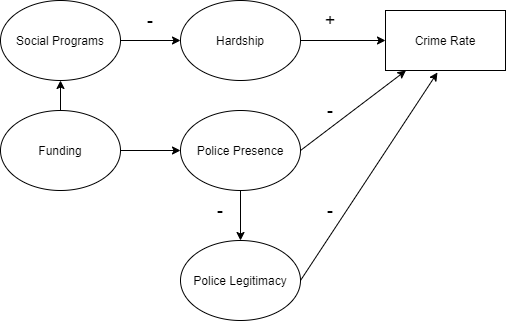
In our conceptual model, we use a term called “hardship,” which is also used by Epstein and Fonoberova et al. Hardship is not well-defined in either those models or in our model, and it is not calibrated on empirical data. In the real world, hardship will correspond to a nonlinear combination of education, income, mental and physical health, and a host of other terms, including interactions between each of them. In our model, it’s just a parameter assigned to the agents, and specifically, it’s the proportion of those factors that lead to an increase in crime.
This conceptual model will be operationalized via an ABM similar to Epstein and Fonoberova et al., but in which both hardship and legitimacy are individual parameters rather than global parameters. Sensitivity analysis will provide insights into specific public policies which might be beneficial.
The purpose of this model is not to be prescriptive to any particular jurisdiction or decision-maker; it is far too simple for that. Rather, it is an exploratory model to evaluate the potential impacts on crime of shifting funding between police and social welfare policies as seen through the lens of police legitimacy and the people’s hardship. This exploration can help inform public policy discussion at a higher level and more detailed decision models can be built from there to capture the specifics of a jurisdiction.
System Model
The layout of this section largely follows the ODD protocol (Overview, Design, Details) for describing Agent-Based Models (Grimm et al. 2020). The goal is to aid in reproducibility to address one of the concerns of Groff et al. (2019).
Model overview
In the model, there are two types of agents placed on a grid: citizens and police. Citizen agents have a “criminal” flag, such that if their “grievance” is above some threshold, the flag is set to “active”. Police move around the grid, and if a police agent sees a criminally-active citizen, the police agent “arrests” the citizen, removing it from the model for a random period of time up to the maximum jail term.
Funding will be shifted between police spending and social spending. Shifting funds to the police and away from social spending increases a “hardship” parameter, which is a factor in determining grievance, but also increases the number of police agents in the grid. Shifting funds in the other direction has the opposite effect.
The model will be run many times with different settings for the funding slider, and the average number of active citizens per day for that run will be recorded (this is a metric used in Fonoberova et al. (2012)).
The model parameters are calibrated on real-world data to address one of the concerns about agent-based models raised by Groff et al. (2019).
Model design and parameters
The citizen agents’ grievance is taken exactly as in Epstein’s (2002) model, that is:
| \[ G = H(1 - L)\] | \[(1)\] |
Hardship and Legitimacy are each set between 0 and 1 in the baseline model for each agent. Hardship represents the portion of Grievance from derived social welfare spending or lack thereof, while Legitimacy is the portion of Grievance affected by police activity.
Citizen agents are also averse to the risk of being arrested. Each citizen agent has a base risk aversion parameter (\(K\)) drawn from a uniform distribution between 0 and 1. A value of 1 indicates that the agent is very risk-averse while a value of 0 indicates that the agent has zero risk aversion. Perceived arrest risk is also impacted by the number of criminals and the number of police in the agent’s vision radius (distance in the number of cells on the grid the agent can use in calculations). Seeing more criminals means a lower arrest risk while seeing more police means a higher arrest risk.
The perceived risk function, as seen in both Epstein (2002) and Fonoberova et al. (2012) is given by:
| \[ P = 1 - e^{\frac{-kC}{A}}\] | \[(2)\] |
The net risk parameter (\(N\)) is a combination of the risk aversion constant and the above risk function, such that:
| \[ N = KP\] | \[(3)\] |
A citizen becomes criminally active when \(G - N > T\), where \(T\) is a criminality threshold, drawn for each agent between 0 and 1. \(T\) represents an individual’s willingness to resort to crime. Someone with a \(T\) of 0 will turn to crime as soon as they have any grievance whatsoever if they don’t think they’ll get caught. Conversely, someone with \(T = 1\) will not turn to crime even with maximum hardship and minimum legitimacy. An active citizen ceases to be active when \(G - N < T\).
So far, all of these parameters have followed Fonoberova et al. (2012) and Epstein (2002). The main difference is that L is a global parameter in those models and a dynamic individual one here. We introduce a few additional parameters. The full list is shown in Table 1.
| Parameter | Description | Value/Range | Source |
|---|---|---|---|
| Hardship (\(H\)) | Baseline hardship. Contributing factor to criminality, affected by social spending | 0 to 1 | Epstein (2002) |
| Legitimacy (\(L\)) | Initial legitimacy. Contributing factor to criminality, affected by police presence | 0 to 1 | Epstein (2002) |
| Risk aversion (\(K\)) | Willingness to become an active criminal when chance of arrest is high | 0 to 1 | Fonoberova et al. (2012) |
| Criminality threshold (\(T\)) | Threshold to determine when a citizen becomes an “active” criminal | 0 to 1 | Epstein (2002) |
| Initial social budget | Initial social budget | $2250 per citizen | Urban Institute (2020), Tax Policy Center (2021) |
| Fraction citizens | What fraction of the grid is populated by citizen agents | 70% | Initial condition similar to Epstein (2002) and Fonoberova et al. (2012) |
| Fraction police | What fraction of the grid is populated by police officers | Determined by police budget, baseline value is 0.36% | Federal Bureau of Investigation (2019b) |
| Legitimacy impact multiplier (\(X\)) | Percentage that legitimacy is decreased when police are active in an area | 0-20% | Sensitivity analysis test parameter |
| Hardship multiplier (\(M\)) | Percent reduction in Hardship as a function of Social spending | 0-100% | Sensitivity analysis test parameter |
| Cost per officer | Annual cost of a police officer | $150000 | See discussion |
| Police vision | Radius of cells that police agents can see | 16 | Initial condition |
| Citizen vision | Radius of cells that citizen agents can see | 14, 16, 18 | Lower, same, and higher than police vision as in Fonoberova et al. (2012) |
| Police | Multiplies the initial police budget | 0-3 | Main test parameter |
| Maximum Jail Term | Maximum jail term for arrested citizens | 30 | Epstein (2002) |
The initial social budget is set at $2250 per citizen agent. This approximates the value we see in the real world, which is roughly $2264 spent per citizen on average on public welfare expenditures (Tax Policy Center 2021; Urban Institute 2020). In principle, we could also have included education and health expenses in this number, since the social budget is what determines “hardship” in our model, and health and education can impact hardship. However, not every dollar spent on public welfare goes to reducing hardship, nor does every dollar spent on education. We assume these effects roughly cancel out and perform sensitivity analysis on this parameter to see how much of an impact this decision has.
The other budgetary parameter we use is the cost per police officer. This also varies by location, but several sources point to a similar range of values. Chicago’s Ward 43 alderman put out a detailed breakdown of the annual cost of a police officer (Chicago Ward 43. 2015), including equipment and supervision, and came up with a value of $149,362. The Boston Police Department has an annual budget of roughly $400 million (City of Boston 2021) and has roughly 2139 uniformed officers (Federal Bureau of Investigation 2019a), leading to an annual cost per officer of around $187,000. Some of these costs will be fixed and some are unrelated to actual policing, so it makes sense that the number is a bit high. Our estimate of $150,000 per officer is in line with what we’d expect in an urban police department. Small deviations from this number didn’t substantially change the behavior of the model.
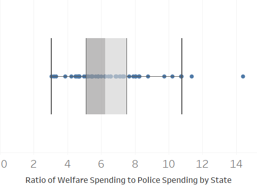
The spending per officer and per citizen need to be multiplied by the number of officers and the number of citizens respectively. We use a grid size of 100 x 100 for 10,000 total cells. 70% are occupied by citizens, for 7000 total. The initial number of police agents is 25, which is 0.36% of the citizen agents. That number lines up closely with the number of police officers per capita in the FBI’s Uniform Crime Reporting data (Federal Bureau of Investigation 2019a). This leads to a baseline budget of $19,500,000, where $15,750,000 is for social welfare and $3,750,000 is for police. The ratio between the two, 4.2, lines up well with real-world data, as seen in Figure 2.
A key part of the model is dynamic legitimacy. When police make an arrest, citizens nearby (determined by their vision) will have their view of legitimacy reduced by the legitimacy impact multiplier. In other words, \(L = L^{'}(1 - X)\).
This isn’t necessarily realistic. Weisburd & Telep (2014) show in their summary article that in some cases police activity increases the view of police legitimacy of the citizens, especially among those with a high view of legitimacy to begin with and among affluent citizens (low hardship). In our model, those with a high view of legitimacy and low hardship are unlikely to become active even if \(L\) decreases by a small percentage. Thus, it doesn’t matter whether \(L\) increases or decreases for them if they don’t become criminally active either way. However, those with a high \(H\), low \(L\), or both (as is often the case in disadvantaged communities), are more likely to become an active criminal when \(L\) is lowered further, and this lines up well with previous research (e.g., Kane (2005)). We perform sensitivity analysis on \(X\), not only to test the robustness of the model but also as a policy lever. As noted earlier, different police tactics can affect the view of police legitimacy, and this parameter gives us a way to model that.
At the end of each tick of the model, half of the missing legitimacy is recovered, meaning:
| \[ L = L + \frac{(L^{'} - L)}{2}\] | \[(4)\] |
This means that occasional encounters with police won’t have a lasting impact, but repeated interactions (as is the case in hot spot policing) will add up over time.
Police vision is set to 16, which means at each step they look in a 16-cell radius to see whether there are any active criminals to arrest. Citizen vision determines net perceived risk and the legitimacy impact of seeing police arrests. Citizen vision was tested at a little lower than, the same as, and a little higher than police vision. This was previously tested by Fonoberova et al. (2012) and found to be significant with regard to the level of crime. With the addition of dynamic legitimacy tied to citizen vision, we expect this to be an important parameter.
The main funding lever is the police budget multiplier. The police budget is determined by the initial police budget ($3,750,000) multiplied by the police budget multiplier. The number of police agents on the grid is equal to the total police budget divided by the cost per officer, rounded down. Increasing the police budget decreases social funding.
As social funding changes, so does hardship. Each agent is assigned a baseline hardship value from 0 to 1, which is then modified by the level of social funding, such that:
| \[ H = H^{'} e^{M(1 - (\frac{SB}{2250})^{2})}\] | \[(5)\] |
where \(SB\) is the social budget per citizen. This is calculated by taking the initial budget of $19,500,000, subtracting the total police budget, and dividing it by 7,000 (the number of citizens). M, the hardship multiplier, is used to test the sensitivity of our model to the assumption that hardship actually changes as the budget changes.
This functional form was chosen so that hardship was bounded as the social budget went to 0. The functional form of \(H = H^{'}(\frac{2250}{SB})\) was also tested, but that leads to infinite hardship as \(SB\) goes to zero.
Model implementation and experimental design
The model was built in NetLogo version 6.2 (Wilensky 1999). We perform global sensitivity analysis (Wagner 1995) using the BehaviorSpace tool within NetLogo. This tool allows us to vary multiple parameters simultaneously. We collect the average number of criminally-active citizens, the average number of jailed citizens, average hardship, and average legitimacy of the citizens for each run.
Each run of the model ran for 100 ticks, which is long enough for the averages to come to an equilibrium. The pseudoavailable is as follows:
- Set police funding and other parameters (e.g. social funding)
- Generate agents on the grid (police and citizen)
- Loop 100 times:
- For each citizen, If citizen \(Grievance -\) \(Net\) \(Perceived\) \(Risk\) \(>\) \(Criminality\) \(Threshold\), become “active”, otherwise inactive
- For each police agent:
- Loop 20 times: If an active citizen is within police vision radius, “arrest” the closest active citizen (set jail term to [0, Max Jail Term])
- Reduce the legitimacy of citizens within citizen vision radius by the legitimacy multiplier
- Else move randomly within police vision radius
- For each citizen, recover half of missing legitimacy
- Recalculate \(Grievance\)
- Increment loop counter
Table 2 shows the parameters which were varied for each run. There were 2,196 combinations of parameters tested.
| Parameter | Range |
|---|---|
| Police funding multiplier | 0-3 in increments of 0.05 |
| Legitimacy Impact multiplier | 0, 0.5, 0.1, 0.2 |
| Citizen Vision | 14, 16, 18 |
| Hardship Multiplier | 0, 0.5, 1 |
We tested the maximum jail term during early runs of the model and found that it had no impact anywhere from 10 to 50, so we kept it at 30 during the main data collection runs. We also tested whether allowing the citizens to move had an impact and found none.
Results
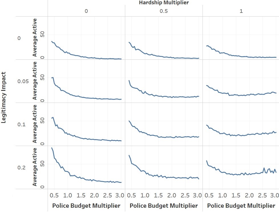
The primary output variable we’re concerned with is the average number of criminally-active citizens per tick, which is a proxy for the crime rate. This was the method used by Fonoberova et al. (2012) to calibrate their model output with FBI crime data. We also consider the average number of citizens in jail per day as a secondary measure. This is a little trickier to tie to a specific real-world value (like the percent of the population that is incarcerated) because our model does not attempt to accurately depict jail terms. However, it does provide insight into how many different citizens commit crimes. For example, in a scenario in which there is a robust social welfare system but a smaller police force, very few people may want to resort to crime, but the ones that do might be harder to catch. On the other hand, in an authoritarian police state with no social welfare system, many people may resort to crime out of desperation but are caught quickly. These situations may end up giving a similar crime rate (or in the model, active citizens per tick), but the reality would be very different, which is why the secondary measure of “average jailed citizens” is used. Figure 3 shows our main results.
There are two ways to interpret this data. The first way, which is most useful for policy-making, is to consider an increase or decrease in funding in one jurisdiction. The second way is to consider differences in funding decisions between jurisdictions. This model was designed with the first interpretation in mind. One benefit of using an ABM is being able to change a policy lever like police funding and keep everything else constant. When comparing different jurisdictions, virtually everything is at least a little different.
We are mainly concerned with the overall shape of the “Average active” curve. Comparing raw numbers across different parameter values isn’t as useful. For example, when legitimacy impact is 0.2, there is simply more crime across all runs compared to when it is 0. However, the crime reduction when going from a budget multiplier of 0.4 to a multiplier of 3 is larger when the legitimacy impact is higher. The shape of the curves changes dramatically as we move from the upper-left corner of Figure 3 to the lower right. When either hardship or legitimacy (or both) is 0, the curves closely fit a power-law relationship. However, when both factors are taken into consideration, a power-law relationship is a very poor match. The best power-law fit generates a 0.984 \(R^{2}\) value for the upper-left graph and only a 0.035 \(R^{2}\) for the bottom-right graph.
Previous research, such as Fonoberova et al. (2012), had output that looked similar to the upper-left chart of Figure 3. As more police were added to the model, crime decreased precipitously. If there were in fact a power-law relationship between police spending and crime, the relation between the two would be much easier to see in empirical studies.
When hardship and legitimacy are taken into account, the curves are much flatter, and therefore the relationship between crime and police spending is much subtler. This flattening mainly occurs when the police budget multiplier is 1.5 or above, which would be a large increase in police funding for a particular jurisdiction. When considering a small change in police funding, say between a 10% decrease and a 10% increase, crime only increases or decreases (respectively) by roughly 3% in the bottom-right graph of Figure 3. Despite the exploratory nature of this model, this value lines up pretty closely with the value of 1.4% in Kovandzic & Sloan (2002).
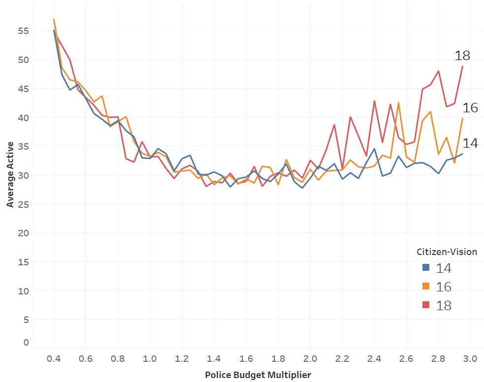
We used a citizen vision value of 16 for the results in Figure 3, meaning both citizen agents can “see” 16 cells away in any direction, but all three values tested were almost identical with one exception. While Fonoberova et al. (2012) found that vision played an important role, the effect was much smaller here. In fact, for the vast majority of runs, citizen vision has no impact. This changed when the police budget multiplier was very high, hardship multiplier was set to 1, and the legitimacy impact was set to 0.2. When a citizen’s vision is greater than the police’s vision where the number of police was very high, crime rates rose (Figure 4).
Instead of just looking at the number of criminally-active citizens, we can also consider the number of people in jail as a metric to determine the effectiveness of budget decisions. Figure 5 shows the same runs as Figure 3 but with the average number of jailed citizens during the run as the dependent variable.
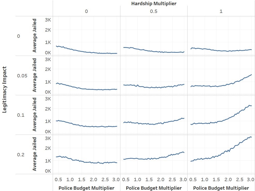
The intuition behind the results in Figure 5 is that the more citizens with a grievance above their criminality threshold, the more people commit crimes. More police officers mean that those active criminals get jailed quickly, and therefore are not active for long, but there are simply a higher number of criminals. When the hardship multiplier and legitimacy impact are 0, there is no increase in grievance, and therefore no increase in criminals as the number of police increases. In fact, the police presence increases the risk of getting arrested and thus prevents citizens with a high grievance from becoming active in the first place. This does not hold when hardship and legitimacy are taken into account. The suppressive effect of having more police cannot keep up with the increase in grievance. Cutting social programs to add more police is counterproductive by this metric under those circumstances.
Post-hoc analysis
One interesting check of the reasonableness of our model is to compare it to empirical data. The difficulty with this, however, is that our model was designed to be different realizations of a single hypothetical jurisdiction, keeping everything else constant. There are too many variables, many interacting in nonlinear ways, to easily compare the impact on crime of funding decisions of different jurisdictions.
That said, a difference between our model and empirical data led to questioning one of the assumptions of the model; that the number of police and the impact on legitimacy per interaction with the police were independent.
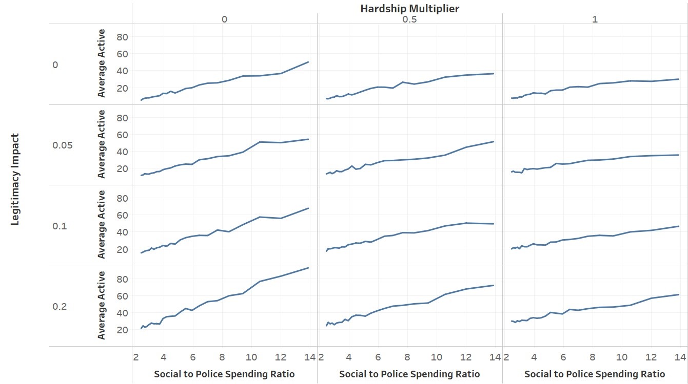
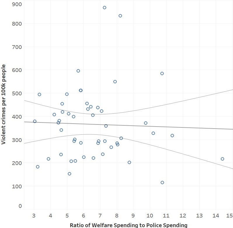
Figure 6 shows our results framed in terms of the ratio between social spending and police spending. Figure 7 shows the same ratio for each US state plotted against the violent crime rate in those states.
The relationship is nearly linear, so to get a clearer picture of the above results, we performed a linear regression in Tableau, and the results are seen in Table 3. There is more crime overall when the legitimacy impact is higher, but within each subset of runs in which the legitimacy impact is held constant, a higher hardship multiplier leads to a flatter relationship between the spending ratio and crime.
| Legitimacy Impact | Hardship Multiplier | Linear coefficient | Standard Error | t-value | p-value |
|---|---|---|---|---|---|
| 0 | 0 | 3.61513 | 0.103748 | 34.8453 | < 0.0001 |
| 0 | 0.5 | 2.81563 | 0.11136 | 25.2841 | < 0.0001 |
| 0 | 1 | 2.17449 | 0.118099 | 18.4124 | < 0.0001 |
| 0.05 | 0 | 4.0493 | 0.120682 | 33.5535 | < 0.0001 |
| 0.05 | 0.5 | 3.09936 | 0.120625 | 25.6942 | < 0.0001 |
| 0.05 | 1 | 2.0549 | 0.113984 | 18.028 | < 0.0001 |
| 0.1 | 0 | 4.51401 | 0.127265 | 35.4695 | < 0.0001 |
| 0.1 | 0.5 | 3.09998 | 0.121379 | 25.5397 | < 0.0001 |
| 0.1 | 1 | 2.30464 | 0.075429 | 30.554 | < 0.0001 |
| 0.2 | 0 | 6.34285 | 0.125712 | 50.4556 | < 0.0001 |
| 0.2 | 0.5 | 4.23944 | 0.121164 | 34.9893 | < 0.0001 |
| 0.2 | 1 | 2.79876 | 0.103947 | 26.9249 | < 0.0001 |
This does not match empirical results when comparing the same spending ratio to violent crime rates for each US state in 2019, as seen in Figure 7. There is simply no relationship between the two without controlling for anything else. This is in line with what Akpom & Doss (2018) found.
As mentioned above, we don’t expect our model to closely match empirical data at this level of analysis since each jurisdiction is a unique complex system, and we were only considering a change in one system with everything else being held constant. When comparing US states, nothing is being held constant. However, this result naturally leads to the question “What would our model need to look like to match the empirical data?”
In our model, we assume that the legitimacy impact of being near a police officer is independent of the number of officers. With many officers, the cumulative impact of interacting with officers leads to a lower legitimacy, but each interaction had the same effect. The intuition behind this assumption is that if more officers are chasing the same or a diminishing number of criminals, the officers may need to bother innocent citizens more often, leading to a larger reduction of legitimacy per interaction. Conversely, if there are few police officers, the interactions they have may be more likely to be seen as legitimate.
To model this, we performed another set of 183 runs in which the legitimacy impact was set to the initial police density (which was the number of police / number of squares in the grid expressed as a percentage), citizen vision was kept at 16, and the rest of the parameters were the same. Thus, if 0.16% of the grid were police officers, the legitimacy impact would be 0.16. This leads to the result seen in Figure 8.
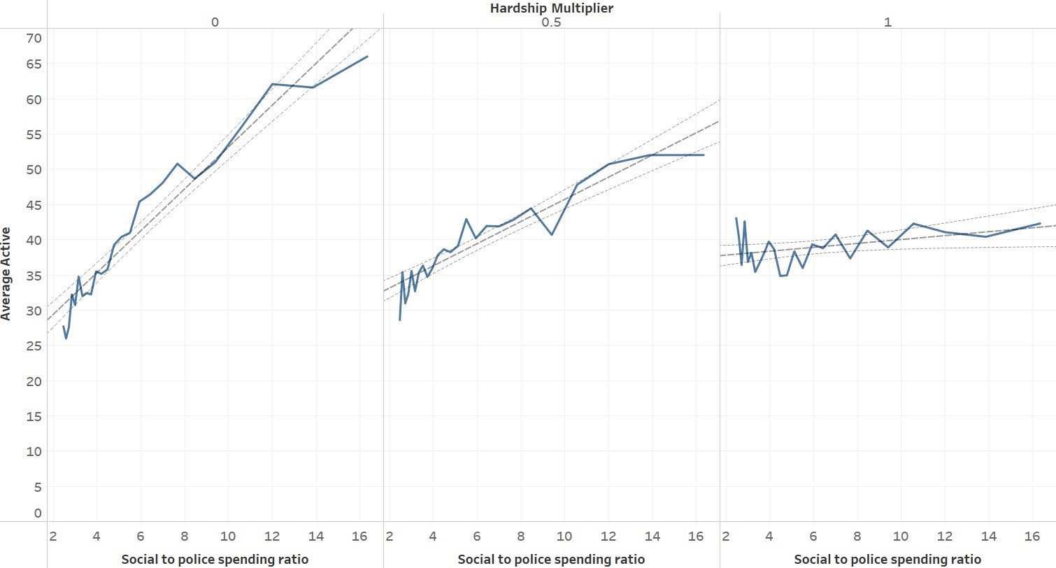
In the case where the hardship multiplier is 1, there is no relationship between the spending ratio and crime in the dynamic legitimacy version of the model.
The decision to reduce police funding to increase social spending is clearer if the jurisdiction in question is better described by this version of the model. This may be the case if there are specific activities by the police that impact legitimacy more than others. Shifting funding from those high legitimacy impact activities to social welfare may be justified.
Discussion
Our results may provide one reason why different funding decisions don’t seem to have a clear impact on crime in the literature. In our model, the crime rate is somewhat insensitive to a large range of funding allocations between police and social spending when hardship and legitimacy are taken into account. Under certain conditions, a dollar spent on either the police or social welfare reduces crime by roughly the same amount. This was an interesting result. We might expect crime to be high when there are no police or there is almost no social funding, so there should be at least one minimum point between the two extremes. The broad, flat area of funding insensitivity was somewhat unexpected.
In our model, this funding insensitivity is particularly prominent when the hardship and legitimacy multipliers are high, or when the legitimacy multiplier is a dynamic value based on police funding as in the post-hoc model. When only hardship or legitimacy is considered separately, this insensitivity is not present. There is a clear decline in crime when police funding is added when considering only hardship or legitimacy; the interaction between the two seems important. This lines up well with Kane (2005) who noted that legitimacy was a predictor of violent crime among disadvantaged populations. If being disadvantaged is interpreted as a hardship in our model, this is the same interaction between hardship and legitimacy our model demonstrates. This further demonstrates that our model can potentially explain empirical results, and thus could have implications for real-world policy levers involving legitimacy and hardship.
The hardship multiplier is related to the efficiency of welfare spending on reducing crime. If real-world social spending is well-targeted to reduce the types of hardship that lead to crime then it correlates to a high hardship multiplier in the model. The legitimacy multiplier is related to public opinion of the police and the willingness of the public to help the police do their jobs. Different police policies and actions may have differing impacts on police legitimacy. In fact, one could imagine a world in which the legitimacy multiplier is negative, meaning interactions with police increase police legitimacy, regardless of starting hardship or legitimacy values.
Combining the above, we conclude that shifting funding away from police activities that have the biggest negative impacts on legitimacy into social funding which has the biggest deterrent on crime could mean either no change in the crime rate or even feasibly a decrease in crime. As each jurisdiction is a unique complex system, as previously described, what might work in one jurisdiction might not work in another.
This naturally leads to the question: “If there is no impact on crime rates, why change funding at all?” The simple answer is that there are more objectives to optimize for in society than the crime rate. Reducing the hardship of its citizens is a reasonable goal for any government. In fact, one interesting question not explored here is to what extent people would actually tolerate an increase in crime in exchange for better social programs.
Conclusions
Revisiting the research questions in the introduction, we find that in our model, what happens to the crime rate when funding is shifted between police and social programs depends on the interaction between legitimacy and hardship. When there is no legitimacy impact of police spending or no hardship impact of social spending, adding more police monotonically reduces crime. However, when both legitimacy and hardship are taken into account, especially when the hardship multiplier is high (meaning the social programs are particularly effective), shifting money away from police to social programs doesn’t have much of an impact on crime rates.
This research has important theoretical and practical implications. Theoretically, this research is a further refinement of Epstein’s (2002) model of civil violence and extends the Fonoberova et al. (2012) application of agent-based modeling to criminology. Where Epstein’s model had hardship and legitimacy as nebulous concepts, we have grounded the two terms in existing criminology research. Notably, we allowed police legitimacy to be heterogeneous and dynamic, which is more realistic and can be an anchor point for future research.
Additionally, our model can help explain the mixed results in empirical criminology research, where neither police spending nor social spending seems to have a clear impact on crime rates. The tradeoff between police and social spending, mediated by the concepts of hardship and legitimacy, can lead to the observed mixed results.
Practically, politicians and administrators can use the insights here as a lens to view their own specific jurisdiction when making budgeting decisions. As they’re deciding what to cut and what to expand, the impact on legitimacy and hardship can help guide their process. For example, if they come across a program or policy that has a large negative impact on police legitimacy (e.g., the “stop and frisk” policy of New York City; Gau & Brunson 2010), scrutiny may be warranted.
This model also demonstrates that there may exist a scenario in which increasing the police budget beyond a certain point can actually increase crime, which is a counterintuitive result. And even if it doesn’t reach that level, there appear to be diminishing returns to simply adding more police. This exploratory model should not be interpreted as prescriptive advice for any particular public policy; rather it shows a plausible interaction between hardship and police legitimacy. A public policy decisionmaker may want to consider these impacts when voting on or implementing new policies or budgets.
Limitations and future research
Our model has some limitations, any of which can lead to opportunities for future research.
In general, this is a very high-level model that cannot provide specific policy recommendations for any specific jurisdiction. A system would need to be modeled in much more detail to be prescriptive. For example, each interaction with police and each crime is considered the same in our model. Different crimes may be impacted by hardship and legitimacy differently, and police interactions may have a heterogeneous impact on legitimacy. There is also a time delay on many interventions. Improving child care or reducing environmental lead may reduce crimes, but it may involve a large lag between when the expenditure is made and when the results are seen.
Another shortcoming is that no attempt was made to model jail terms in any realistic way. This model could in theory be used to examine the effectiveness of different incarceration policies. When a citizen in our model is released from prison, they’re released with the same legitimacy, hardship, risk aversion, and criminality threshold parameters as they went in. In real life, prison might change a person, for good or for ill. This model could be adapted to explore the impacts of prison reform on crime.
One other possibility, as mentioned in Section 6, is to consider the tradeoff between the objectives of reducing crime and providing for the general welfare of the population. People may have differing political opinions and worldviews about what amount of financial hardship is equivalent to the hardship of being the victim of a crime. For example, is it worse to have $100 stolen from you, or to lose $100 in benefits? A version of this model could be used to explore that tradeoff.
Model Documentation
The full model is available on COMSeS Net and can be downloaded at: https://www.comses.net/codebases/60a21669-865b-4ab6-a59d-93f980f89901/releases/1.0.0/
References
AKPOM, U. N., & Doss, A. D. (2018). Estimating the impact of state government spending and the economy on crime rates. Journal of Law and Conflict Resolution, 10(2), 9–18.
AMERICAN Civil Liberties Union. (2020). Defunding the police will actually make us safer. Archived at: https://web.archive.org/web/20220425145817/https://www.aclu.org/news/criminal-law-reform/defunding-the-police-will-actually-make-us-safer.
BUREK, M. W. (2005). Now serving part two crimes: Testing the relationship between welfare spending and property crimes. Criminal Justice Policy Review, 16(3), 360–384. [doi:10.1177/0887403405274782]
CHICAGO Ward 43. (2015). Full cost of a police officer. Archived at: https://web.archive.org/web/20211009021842/https://ward43.org/wp-content/uploads/2015/09/Cost-per-Police-Officer_vF.pdf.
CITY of Boston. (2021). Current and past fiscal year budgets. Available at: https://www.boston.gov/departments/budget#current-and-past-fiscal-year-budgets.
DAHL, R. A. (2020). On democracy. New Haven, CT: Yale University Press.
DEFRONZO, J. (1983). Economic assistance to impoverished Americans. Criminology, 21, 119–136.
DEFRONZO, J. (1996). Welfare and burglary. Crime & Delinquency, 42, 223–229. [doi:10.1177/0011128796042002004]
DONOHUE III, J. J., & Siegelman, P. (1998). Allocating resources among prisons and social programs in the battle against crime. The Journal of Legal Studies, 27(1), 1–43. [doi:10.1086/468012]
EAGLIN, J. M. (2020). To "Defund" the police. Stanford Law Review Online, 73, 120.
EPSTEIN, J. M. (2002). Modeling civil violence: An agent-based computational approach. Proceedings of the National Academy of Sciences, 99(3), 7243–7250. [doi:10.1073/pnas.092080199]
ESTRADA, M. A. R. (2011). Policy modeling: Definition, classification and evaluation. Journal of Policy Modeling, 33(4), 523–536.
FEDERAL Bureau of Investigation. (2019a). Crime in the U. S. Uniform Crime Report. Available at: https://ucr.fbi.gov/crime-in-the-u.s/2019/crime-in-the-u.s.-2019/topic-pages/tables/table-5.
FEDERAL Bureau of Investigation. (2019b). Full-time law enforcement employees. Uniform Crime Report. Available at: https://ucr.fbi.gov/crime-in-the-u.s/2019/crime-in-the-u.s.-2019/tables/table-74.
FONOBEROVA, M., Fonoberov, V. A., Mezic, I., Mezic, J., & Brantingham, P. J. (2012). Nonlinear dynamics of crime and violence in urban settings. Journal of Artificial Societies and Social Simulation, 15(1), 2. [doi:10.18564/jasss.1921]
GAU, J. M., & Brunson, R. K. (2010). Procedural justice and order maintenance policing: A study of inner‐city young men’s perceptions of police legitimacy. Justice Quarterly, 27(2), 255–279. [doi:10.1080/07418820902763889]
GRIMM, V., Railsback, S. F., Vincenot, C. E., Berger, U., Gallagher, C., DeAngelis, D. L., Edmonds, B., Ge, J., Giske, J., Groeneveld, J., Johnston, A. S. A., Milles, A., Nabe-Nielsen, J., Polhill, J. G., Radchuk, V., Rohwäder, M. S., Stillman, R. A., Thiele, J. C., & Ayllón, D. (2020). The ODD protocol for describing agent-based and other simulation models: A second update to improve clarity, replication, and structural realism. Journal of Artificial Societies and Social Simulation, 23(2), 7. [doi:10.18564/jasss.4259]
GROFF, E. R., Johnson, S. D., & Thornton, A. (2019). State of the art in agent-based modeling of urban crime: An overview. Journal of Quantitative Criminology, 35(1), 155–193. [doi:10.1007/s10940-018-9376-y]
HAWDON, J. E., Ryan, J., & Griffin, S. P. (2003). Policing tactics and perceptions of police legitimacy. Police Quarterly, 6(4), 469–491. [doi:10.1177/1098611103253503]
KANE, R. J. (2005). Compromised police legitimacy as a predictor of violent crime in structurally disadvantaged communities. Criminology, 43(2), 469–498. [doi:10.1111/j.0011-1348.2005.00014.x]
KOLLIAS, C., Mylonidis, N., & Paleologou, S. M. (2013). Crime and the effectiveness of public order spending in Greece: Policy implications of some persistent findings. Journal of Policy Modeling, 35(1), 121–133. [doi:10.1016/j.jpolmod.2012.02.004]
KOVANDZIC, T. V., & Sloan, J. J. (2002). Police levels and crime rates revisited: A county-level analysis from Florida (1980-1998). Journal of Criminal Justice, 30(1), 65–76. [doi:10.1016/s0047-2352(01)00123-4]
MACAL, C. M., & North, M. J. (2005). Tutorial on agent-based modeling and simulation. Proceedings of the Winter Simulation Conference (pp. 14-pp). IEEE [doi:10.1109/wsc.2005.1574234]
MAZEPUS, H., & van Leeuwen, F. (2020). Fairness matters when responding to disasters: An experimental study of government legitimacy. Governance, 33(3), 621–637. [doi:10.1111/gove.12440]
MCEVOY, J. (2020). At least 13 cities are defunding their police departments. Forbes. Archived at: https://web.archive.org/web/20220425150714/https://www.forbes.com/sites/jemimamcevoy/2020/08/13/at-least-13-cities-are-defunding-their-police-departments/.
MOULE Jr, R. K., Burruss, G. W., Parry, M. M., & Fox, B. (2019). Assessing the direct and indirect effects of legitimacy on public empowerment of police: A study of public support for police militarization in America. Law & Society Review, 53(1), 77–107. [doi:10.1111/lasr.12379]
OTTERBEIN, H. (2021). A conversation that needs to happen: Democrats agonize over ’defund the police’ fallout. Available at: https://www.politico.com/news/2021/03/23/defund-the-police-democrats-477609.
PEYTON, K., Sierra-Arévalo, M., & Rand, D. G. (2019). A field experiment on community policing and police legitimacy. Proceedings of the National Academy of Sciences, 116(40), 19894–19898. [doi:10.1073/pnas.1910157116]
R., D., & Schargrodsky, E. (2004). Do police reduce crime? estimates using the allocation of police forces after a terrorist attack. American Economic Review, 94(1), 115–133.
RINEHART Kochel, T. (2011). Constructing hot spots policing: Unexamined consequences for disadvantaged populations and for police legitimacy. Criminal Justice Policy Review, 22(3), 350–374. [doi:10.1177/0887403410376233]
ROSENBAUM, D. P. (2006). The limits of hot spots policing. Police Innovation: Contrasting Perspectives, 245–263. [doi:10.1017/cbo9780511489334.013]
SAVAGE, J., Bennett, R. R., & Danner, M. (2008). Economic assistance and crime: A cross-national investigation. European Journal of Criminology, 5(2), 217–238. [doi:10.1177/1477370807087645]
TAX Policy Center. (2021). State and local general expenditures, per capita. Available at: https://www.taxpolicycenter.org/statistics/state-and-local-general-expenditures-capita.
THUNE, J. (2021). Demonizing and defunding police has consequences. Archived at: http://web.archive.org/web/20230322203350/https://www.thune.senate.gov/public/index.cfm/2021/7/demonizing-and-defunding-police-has-consequences.
TYLER, T. R., & Fagan, J. (2008). Legitimacy and cooperation: Why do people help the police fight crime in their communities. Available at: https://scholarship.law.columbia.edu/faculty_scholarship/414/. [doi:10.2139/ssrn.887737]
URBAN Institute. (2020). Public welfare expenditures. Archived at: https://web.archive.org/web/20220425151520/https://www.urban.org/policy-centers/cross-center-initiatives/state-and-local-finance-initiative/state-and-local-backgrounders/public-welfare-expenditures.
WAGNER, H. M. (1995). Global sensitivity analysis. Operations Research, 43(6), 948-969.
WALLNER, J. (2008). Legitimacy and public policy: Seeing beyond effectiveness, efficiency, and performance. Policy Studies Journal, 36(3), 421–443. [doi:10.1111/j.1541-0072.2008.00275.x]
WEISBURD, D., & Telep, C. W. (2014). Hot spots policing: What we know and what we need to know. Journal of Contemporary Criminal Justice, 30(2), 200–220. [doi:10.1177/1043986214525083]
WILENSKY, U. (1999). NetLogo. Center for Connected Learning and Computer-Based Modeling, Northwestern University, Evanston, IL. Available at: http://ccl.northwestern.edu/netlogo/.