Spatial Disparities in Vaccination and the Risk of Infection in a Multi-Region Agent-Based Model of Epidemic Dynamics

and
aCleveland State University, United States; bFordham University, United States
Journal of Artificial
Societies and Social Simulation 26 (3) 3
<https://www.jasss.org/26/3/3.html>
DOI: 10.18564/jasss.5095
Received: 26-Nov-2022 Accepted: 30-Mar-2023 Published: 30-Jun-2023
Abstract
We investigate the impact that disparities in regional vaccine coverage have on the risk of infection for an unvaccinated individual. To address this issue, we develop an agent-based computational model of epidemics with two features: 1) a population divided among multiple regions with heterogeneous vaccine coverage; 2) contact networks for individuals that allow for both intra-regional interactions and inter-regional interactions. The benchmark version of the model is specified using county-level flu vaccination claims rates from California. We isolate the effects of heterogeneity by holding overall vaccination levels constant, while changing the variance in the distribution of regional vaccine coverage. We find that an increase in spatial heterogeneity leads to larger epidemics on average. This effect is magnified when more connections that are inter-regional exist in the contact structure of the networks. The central result in the paper is that there is a non-monotonic relationship between the infection risk and the geographic resolution of vaccination rate measurement. Infection risk of an unvaccinated individual decreases in both the global rate of vaccinations and the rate of vaccination of the individual’s specific contacts. Surprisingly, we find that the vaccination rate in an individual’s home region does not have a significant impact on an individual’s infection risk in our model. This has significant implications for an individual’s vaccine choices. Global and local (network specific) vaccination rates are highly correlated with infection risk and thus should be prioritized as information sources for rational decision-making. Using the region-specific information, however, is likely to lead to non-optimal decisions.Introduction
In recent years, there is growing concern over the spatial heterogeneity of vaccine coverage. The concern grew when recent measles outbreaks in the United States and Europe were traced to pockets of unvaccinated children (CDC 2023). The uneven distribution of the COVID-19 vaccine in developing countries as well as across geographic locations in the United States and Europe has made the issue even more important in both academic and policy discussions.
In particular, the issue of the anti-vaccine movement has sparked a wide spread discussion in academics (Buttenheim et al. 2012; Poland & Jacobson 2001) and the general press (Ingraham 2015; Oster & Kocks 2018). Some of these discussions focus on rates of vaccination refusal in particular locations and the correlation with epidemic size within these locations (Atwell et al. 2013; Feikin et al. 2000). Many other studies examine the demographic correlates of vaccine refusal and try to identify factors that lead to anti-vaccine sentiment or refusal (Atwell et al. 2013; Birnbaum et al. 2013; Gust et al. 2004; McNutt et al. 2016; Sugarman et al. 2010).
Despite the publicity received by this movement, overall levels of vaccination rates have not changed significantly in the years leading up to the COVID-19 pandemic. For example, the US vaccination rate for Measles Mumps and Rubella (MMR) has been relatively stable for two decades. Rates of MMR vaccination for children 19-35 months old have been between 89.7% and 93.0% from 1995 until 2017. Since 2000 the rates are in an even narrower range between 90.0% and 92.1% (with the low in 2009 and the high in 2008.) (CDC 2018). More recently, the CDC estimate of the MMR vaccination rate for entering kindergarten students in the 2021-2022 school year sits at 93.0% (Seither et al. 2023). However, while overall rate of vaccine coverage has not changed dramatically in recent years, there exists an interesting and less discussed feature of vaccine coverage: spatial heterogeneity with vaccine refusal being especially high in particular localized areas (Carrel & Bitterman 2015; Lieu et al. 2015; May & Silverman 2003). As a macro-level example, the MMR coverage data discussed above has a wide variety of vaccine coverage at the state level. In 2017, the state with the lowest MMR coverage was Missouri with just under 86% coverage; Massachusetts, the state with the highest level of coverage, had over 98% coverage.
The wide variation in vaccine coverage across geographic space is not just limited to MMR. A case in point is the influenza vaccine coverage in US. For 2018-19 season, the mean coverage rate for the US was 49.2% with the minimum and the maximum at the state level being 37.8% (Nevada) and 60.4% (Rhode Island), respectively. Table 1 provides the historical data for the period of 2010-2019 as reported by Center for Disease Control (CDC). It is clear that the wide variation in vaccine coverage has persisted over time.
| Season | US % | CI | Min state | Max state |
|---|---|---|---|---|
| 2018-19 | 49.2 | (\(\pm\)0.3) | 37.8 | 60.4 |
| 2017-18 | 41.7 | (\(\pm\)0.3) | 35.3 | 50.1 |
| 2016-17 | 46.8 | (\(\pm\)0.5) | 36.1 | 55.4 |
| 2015-16 | 45.6 | (\(\pm\)0.4) | 36.8 | 56.6 |
| 2014-15 | 47.1 | (\(\pm\)0.3) | 39.2 | 59.6 |
| 2013-14 | 46.2 | (\(\pm\)0.4) | 36.4 | 57.4 |
| 2012-13 | 45.0 | (\(\pm\)0.4) | 34.1 | 57.5 |
| 2011-12 | 41.8 | (\(\pm\)0.4) | 32.6 | 51.1 |
| 2010-11 | 43.0 | (\(\pm\)0.4) | 36.5 | 55.6 |
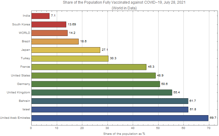
Another case in point, though at a much larger scale, are the current COVID-19 vaccine rates. The prevailing scientific view is that the wide disparities between countries in vaccine availability and its distribution as well as vaccine refusal are among the major determinants of the evolving rates of disease at both national and global levels (Aschwanden 2021). Figure 1 plots the share of the population fully vaccinated against COVID-19 as of July 28, 2021 for a select group of countries. The wide disparities in vaccine distribution even in this limited sample are quite striking as we observe the percentage shares ranging from 7.1% for India to 69.7% for United Arab Emirates with the global average (WORLD) being only around 14.2% - largely driven by low vaccine rates in very populated countries such as India.
All of these observations lead us to the following question: Does spatial heterogeneity in vaccine coverage, independent of the overall level, affect the dynamic and the ultimate severity of the epidemic? If so, what are the implications for the assessment of an unvaccinated individual’s risk of infection as measured at different levels of information aggregation such as global, regional, or individual network-specific infection rates?
These questions can be partially answered using the standard analytical models that exist in the epidemiology literature such as the SIR model. However, the inherent complexities in the structure of the web of contact networks through which an infectious disease may propagate present a substantial barrier to gaining further insights strictly within an analytical framework. In this paper, we propose to explore the issues identified above by developing an agent-based computational model of an epidemic process in a population distributed across geographic regions, in which individuals interact through their intra- and inter-regional contact networks. The benchmark model specifies the distribution of the regional vaccine coverage using the county-level flu vaccination claims rates from California. In order to isolate the effect of only spatial heterogeneity we change the variance in the distribution of vaccination coverage across regions while holding the population level vaccination rate constant. By isolating the variance apart from overall vaccination coverage, we can better understand how regions with low levels of vaccination coverage affect the overall epidemic process and how vaccine refusal by a collection of individuals in the same location affects regional and network based neighbors.
We find that spatial heterogeneity by itself increases epidemic size on average. The effect is larger when there are more inter-regional connections in the contact network. We also examine the infection risk of an individual (the likelihood that an unvaccinated individual is infected) as a function of global and regional rates of vaccination. Not surprisingly, we find that increases in global vaccination rates decrease both epidemic size and individual infection risk. Surprisingly, we find that the vaccination rate of a region is uncorrelated with the infection risk of individuals in the region, even though regions with low vaccination rates have larger epidemics on average. However, infection risk of an individual is negatively correlated with the number of unvaccinated direct network contacts. Thus, in our model, there exists a non-monotonic relationship in the resolution of vaccine coverage and individual infection risk. Macro level and individual level measures of vaccine coverage are good predictors of individual infection risk. But vaccination coverage at an intermediate (regional) resolution may not be closely tied to likelihood of infection. This result has important policy considerations. Individuals who use regional (e.g., school district, neighborhood, or community) levels of vaccinations are unlikely to make accurate predictions of their infection risk. Thus, they are not likely to make optimal decisions with regard to vaccine usage.1
Network based computational and mathematical models of disease transmission, similar to the one implemented in this paper, are frequently used to understand epidemic processes (Epstein 2009; Eubank et al. 2004). These models are used in a variety of ways. In some instances, computational models are used to predict epidemic outcomes as they progress (Tizzoni et al. 2012). The majority aim to investigate epidemic outcomes as a function of complex network variables and behavioral or interaction based assumptions of agents within these models (see, for example, Smith et al. 1999; Bansal et al. 2006; Barrat et al. 2010; Del Valle et al. 2013; Germann et al. 2006; Gersovitz 2013; Stroud et al. 2007; Tassier et al. 2017; Vardavas & Marcum 2013). The unique contribution of our paper is proposing a model that explicitly separates the effect of changes in spatial vaccine coverage heterogeneity from changes in population level vaccination coverage.
Standard \(SIR\) Model of Infectious Disease
One of the simplest mathematical models of disease spread is the SIR model. It belongs to a class of models referred to as compartmental models. In these models, the population is assigned to compartments representing specific states such as \(S\) (susceptible), \(I\) (infectious), or \(R\) (recovered). Individuals can move between compartments as their state changes. The name of the model typically indicates the order of flow between compartments. For example, the \(SIR\) model implies a typical individual moves from susceptible state, \(S\), to infectious state, \(I\), and then to recovered state, \(R\). In most applications, the \(SIR\) model is constructed to capture the disease spread for a single population in a perfectly closed region. In section 2.1, we provide a brief description of such a standard single-region \(SIR\) model. Given our interest in this paper of studying the spread of disease in a multi-regional framework, we then provide, in section 2.2, a limited extension of the SIR model in which the population is distributed between two regions. While this simple extension gives us a clear view of the specific ways in which the added region may influence the epidemic dynamics, the complex interaction across even more regions undermines analytical tractability and severely limits the scale and scope of our investigation. The agent-based model proposed in this paper is meant to surmount the difficulty of analyzing a many region model by agentizing the standard \(SIR\) model in a general multi-regional setting and performing a computational analysis of the epidemic dynamics.
It should be noted that the \(SIR\) model described in this section is the simplest possible analytical model of infectious disease, and our intention here is to show that even within this simple setup the consideration of multi-regional infection spread can significantly raise the level of analytical complexity. Once the number of regions rises above two, the analytical tractability is difficult to sustain and a computational modeling approach becomes the only viable option. As such, the purpose of the discussions in this section are to “motivate” and “justify” the use of our agent-based modeling approach rather than to engage in a direct comparative analysis of the two approaches.
Single-region \(SIR\) model
The discrete time version of the usual \(SIR\) model for a single isolated population takes the following form:
| \[ S(t+1) = S(t) - C T S(t) \frac{I(t)}{N}\] | \[(1)\] |
| \[ I(t+1) = I(t) + C T S(t) \frac{I(t)}{N} - (\frac{1}{D}) I(t)\] | \[(2)\] |
| \[ R(t+1) = R(t) + (\frac{1}{D}) I(t)\] | \[(3)\] |
The most important measure in the standard \(SIR\) model is the basic reproduction number, \(R_{0}\), which is the average number of people a typical infected person can infect when the entire population is susceptible. In our framework, this implies:
| \[ R_{0}= C T D\] | \[(4)\] |
A related concept is the "effective reproduction number," \(R\), which is defined as the average number of people a typical infected person can infect in a given period \(t\) when there are a fraction \(\frac{S(t)}{N}\) of susceptible people in the population:
| \[ R = R_{0} \frac{S(t)}{N}\] | \[(5)\] |
Another notable measure is the "herd immunity threshold," \(h(t)\), which is the proportion of the population that need to be immune in order to prevent an infectious disease outbreak within a region. Note that this level is attained when each case of infection leads to exactly one (or fewer) new case in the standard model such that \(R=1\). Or, \(R=R_{0} \frac{S(t)}{N} = 1\). Since the fraction of susceptible individuals is then \(\frac{S(t)}{N} = \frac{1}{R_{0}}\), the herd immunity threshold takes the following form:
| \[ h(t)=1 - \frac{1}{R_{0}}\] | \[(6)\] |
Two-Region \(SIR\) Model
Suppose now that the population of \(N\) individuals is divided into two spatially distinct regions, 1 and 2, such that each individual belongs to only one of the two regions. Hence, we have \(N= N_{1} + N_{2}\), where \(N_{i}\) is the number of individuals belonging to region \(i\) (\(i=1,2\)).
An individual mainly interacts with other individuals in his/her own home region, but there is always some possibility that he/she may be exposed to someone from the foreign region. To be specific, let us denote by \(\beta\) the probability that an individual is in contact with another individual from the home region; hence, the same individual can come into contact with another person from the foreign region with a probability \(1 - \beta\).
The original \(SIR\) model can be extended to describe the epidemic process in the two-region case. Using the subscripts to denote the two regions, we may write the two-region version of the \(SIR\) model as follows:
| \[ S_{k}(t+1) = S_{k}(t) - C T S_{k}(t) [\beta \frac{I_{k}(t)}{N_{k}} + (1 - \beta) \frac{I_{\overline{k}}(t)}{N_{\overline{k}}}]\] | \[(7)\] |
| \[ I_{k}(t+1) = (1 - \frac{1}{D}) I_{k}(t) + C T S_{k}(t) [\beta \frac{I_{k}(t)}{N_{k}} + (1 - \beta) \frac{I_{\overline{k}}(t)}{N_{\overline{k}}}]\] | \[(8)\] |
| \[ R_{k}(t+1) = R_{k}(t) + (\frac{1}{D}) I_{k}(t)\] | \[(9)\] |
For expositional and analytical simplicity, we may rewrite the above equations in terms of the regional rates (instead of numbers) of susceptibility, infection, and recovery (for regions 1 and 2) such that:
| \[ s_{k}(t+1) = s_{k}(t) - C T s_{k}(t) [\beta i_{k}(t) + (1 - \beta) i_{\overline{k}}(t)]\] | \[(10)\] |
| \[ i_{k}(t+1) = (1 - \frac{1}{D}) i_{k}(t) + C T s_{k}(t) [\beta i_{k}(t) + (1 - \beta) i_{\overline{k}}(t)]\] | \[(11)\] |
| \[ r_{k}(t+1) = r_{k}(t) + (\frac{1}{D}) i_{k}(t)\] | \[(12)\] |
The first property we can identify from the two-region \(SIR\) model is that the impact of \(\beta\) on the infection rate of a given region depends on its current rate of infection relative to that of its neighbor:
| \[ i_{k}(t+1)|_{\beta < 1} \gtreqless i_{k}(t+1)|_{\beta = 1}\] | \[(13)\] |
Hence, cross-regional contacts adversely affects a region if its regional rate of infection is lower than that of the neighboring region, and vice versa. Furthermore, once the cross-regional contact is allowed so that \(\beta < 1\), the size of \(\beta\) similarly affects the regional rate of infection:
| \[ \frac{\partial i_{k}(t+1)}{\partial \beta} \gtreqless 0\] | \[(14)\] |
The main insight here is that the cross-regional contact affects the more infected region favorably and the less infected region adversely. Hence, we may view the cross-regional spillover as a negative externality for the currently safer region and as a positive externality for the less safe region.
We have, thus far, focused on the epidemic implications for each individual region. A bigger question is how cross-regional contacts may affect the spread of the infectious disease at the global level. In other words, how does \(\beta\) affect \(i(t+1)\), where \(i(t+1)= \frac{I_{1}(t+1) + I_{2}(t+1)}{N}\)? The answer to this question is not straightforward, as multi-regional contacts create a positive externality for one region, while they simultaneously create a negative externality for the other region. If these countervailing effects are equal in magnitudes, they may neutralize each other and have no consequence for the global epidemic. But there is no reason to assume that the effects are equally strong. As such, we specifically look at the global infection rate next.
For expositional ease, we express the division of the global population between the two regions using a proportion \(\alpha\) such that \(N_{1} = \alpha N\) and \(N_{2} = (1 - \alpha) N\). The global rate of infection may be written as \(i(t+1)= \alpha i_{1} (t+1)+(1 - \alpha) i_{2} (t+1)\) such that:
| \[ \begin{split} i(t+1) = (1 - \frac{1}{D}) i(t) + C T [i_{1}(t) \{\alpha \beta s_{1} (t) + (1 - \alpha) (1 - \beta) s_{2}(t)\} + & \\ i_{2} (t) \{(1 - \alpha) \beta s_{2} (t) + \alpha (1 - \beta) s_{1}(t)\}] \end{split}\] | \[(15)\] |
When there is no cross-regional contact such that \(\beta = 1\), the equation simplifies to:
| \[ i(t+1)|_{\beta = 1} = (1 - \frac{1}{D}) i(t) + C T \{ \alpha i_{1}(t) s_{1} (t) + (1 - \alpha) i_{2}(t) s_{2}(t)\}\] | \[(16)\] |
We observe the following property when comparing the global infection rate with and without the cross-regional contacts:
| \[ i(t+1)|_{\beta < 1} \gtreqless i(t+1)|_{\beta = 1}\] | \[(17)\] |
This property indicates that the impact of the cross-regional contacts on the global rate of infection depends both on the ratio of the regional infection rate, \(\frac{i_{1}(t)}{i_{2}(t)}\), and the ratio of the regional susceptibility rates, \(\frac{s_{1}(t)}{s_{2}(t)}\). The exact nature of the dependence may be stated as follows:
- Cross-regional contact raises the global infection rate if \(\{\frac{i_{1}(t)}{i_{2}(t)} < 1 \; and \; \frac{s_{1}(t)}{s_{2}(t)} > \frac{1 - \alpha}{\alpha}\}\) or \(\{\frac{i_{1}(t)}{i_{2}(t)} > 1 \; and \; \frac{s_{1}(t)}{s_{2}(t)} < \frac{1 - \alpha}{\alpha}\}\)
- Cross-regional contact reduces the global infection rate if \(\{\frac{i_{1}(t)}{i_{2}(t)} > 1 \; and \; \frac{s_{1}(t)}{s_{2}(t)} > \frac{1 - \alpha}{\alpha}\}\) or \(\{\frac{i_{1}(t)}{i_{2}(t)} < 1 \; and \; \frac{s_{1}(t)}{s_{2}(t)} < \frac{1 - \alpha}{\alpha}\}\)
- Cross-regional contact has no impact on the global infection rate if \(\frac{i_{1}(t)}{i_{2}(t)} = 1\) or \(\frac{s_{1}(t)}{s_{2}(t)} = \frac{1 - \alpha}{\alpha}\)
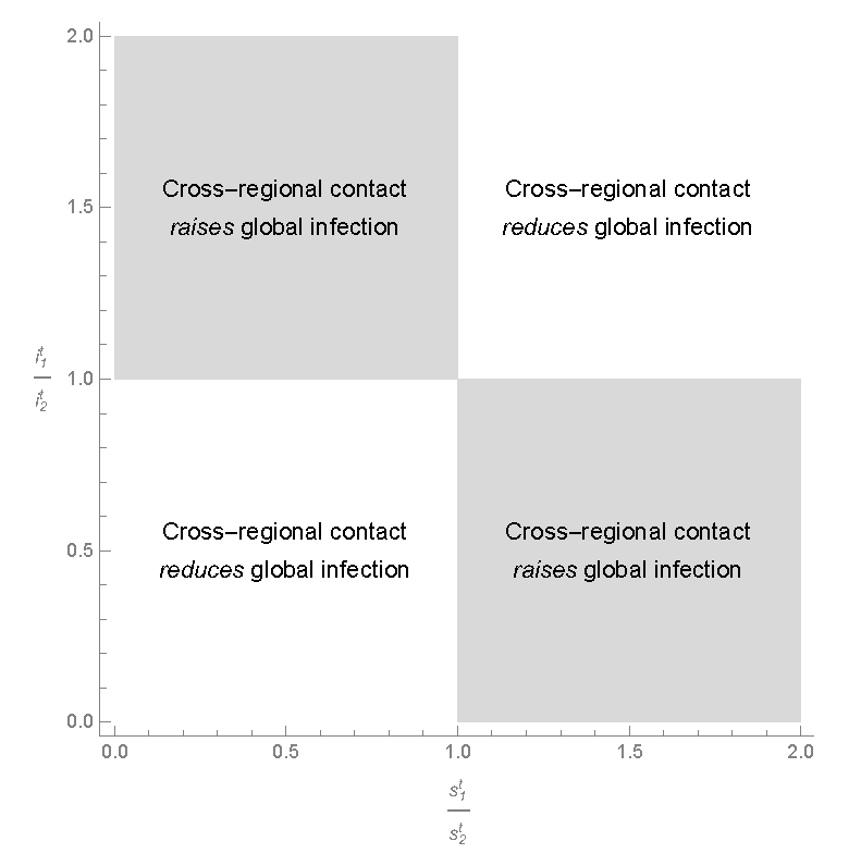
It is instructive to consider a special case where the two regions are of equal size so that \(\alpha = \frac{1}{2}\). In this case, the above property can be visualized as in Figure 3, where the space of the two ratios is divided into four areas with the corresponding property for each area. We can summarize the results as follows:
- The cross-regional contacts raise global infection if a given region has a higher (lower) infection rate but a lower (higher) susceptibility rate;
- The cross-regional contacts reduce global infection if one of the two regions has both a higher rate of infection and a higher rate of susceptibility;
- The cross-regional contacts have no impact on global infection if either the infection rates or the susceptibility rates are equal between the two regions.
Intuitively, the condition for the first case allows cross-regional infection to take place easily from the highly infected region to the highly susceptible region. In contrast, the condition for the second case implies that both infection and susceptibility are concentrated in one region; hence, the cross-regional contacts, by promoting interaction of the individuals from the region with higher infection to the other region with more immune population, result in reducing the global rate of infection.
Agentizing the model of epidemics
There have been many extensions pursued in the analytical tradition so as to treat different types of infectious diseases – e.g., \(SEIR\) model, \(SIS\) model, etc. However, as shown above, a simple extension of the standard \(SIR\) model to include a second region already introduces a substantial degree of complexity to the analysis, significantly limiting the range of questions that can be asked.2 Retaining sufficient analytical tractability typically requires making strong assumptions on the nature of interactions between individuals that influence the contact and transmission rates as well as the state of vaccination in specific regions – e.g., uniform contact probabilities with respect to the rest of the population and homogeneous vaccination across all regions. When the research questions of interest involve spatially defined interactions that require differentiating between the contacts in terms of their proximity or of the nature of their relationships to the given individual, the assumptions needed for tractability become untenable.
In order to circumvent this obstacle without compromising the integrity of our research objective, we propose in this paper an agent-based model of infection spread, which is rooted in the standard \(SIR\) model but is also capable of capturing the complex interactions between individuals from the bottom up. We accomplish this by foregoing the purely analytical methodology and pursuing in its stead a computational model and analysis of the changes in the states of individuals over time. This trade-off is worthwhile in view of the expanded scope of investigation thus achieved. In the next section, we present the agent-based model of epidemics and show how such a formulation expands the space of parameters that we can examine for richer analysis.
A significantly simplified version of our agent-based model was presented in Chang & Tassier (2021) as the first step toward agentizing the multi-regional infection dynamics. In that paper, the authors made a simplifying assumption that all regions are separated into two groups based on two fixed vaccination rates – high vaccination regions (with the vaccination rate fixed at a high level) and low vaccination regions (with the vaccination rate fixed at a low level). It was, hence, a two-region model in essence. This simplification allowed them to focus on the precise details of how the positive externality and the negative externality arise from the inter-regional contacts between the two types of regions as infection spreads across regions. In contrast, our model in the current paper is a “generalized” version of the multi-region model where the regional vaccination rates are specified using a beta distribution across all regions (100 regions in our experiments). The use of a beta distribution is motivated by and specified on the basis of the empirical data on the county-level flu vaccination claims rates from California. This refinement allows us to gain insights of sufficient generality into the relationship between the rates of vaccination and the risk of infection at the individual network level, regional level, and the global level.
Agent-Based Model
The agent-based model presented here is a bottom-up version of the standard \(SEIR\) model, where an individual moves between four states of susceptible (\(S\)), exposed (\(E\)), infectious (\(I\)), and recovered (\(R\)).3 A substantially simplified two-region version of this model was presented in Chang & Tassier (2021). The model presented in this paper is a generalized version, which allows the number of regions to be more realistically large. We combine this model with data from the US Department of Health and Human Services (HSS) on Medicare fee for service beneficiaries. We then run a series of computational simulations over the parameter space of the model.4
A brief description of the model is presented in Appendix A in a format that follows the ODD protocol as proposed by Grimm et al. (2006), Grimm et al. (2010) and Grimm et al. (2020). The following discussion in the remaining part of this section offers a full description of the model.
The infection dynamics modelled in this paper are loosely based on the seasonal influenza virus. In our model an infectious disease propagates over a complex web of interconnected contact networks. We assign agents in the model to one of a set of non-overlapping regions. The regions may be thought of as geographic areas where most person-to-person interactions take place within the area. Each agent is connected to a subset of other agents in the population. Most of the contacts come from the agent’s own region (local contacts) but a small percentage come from outside the agent’s region (global contacts). A region in our model is, hence, defined by the characteristics of the individual contact networks, where the individuals within a given region have higher probability of physical interaction with one another than with those outside of the region. Examples would include school districts with the children having higher rates of contact with other children in the same school district or local communities within which people reside and maintain social interactions through churches, workplaces, and local social gathering places.5
In this paper, agents are assigned a vaccination status exogenously based on the rate of vaccine coverage in their region. We then allow an epidemic process to propagate across the network. By holding the mean vaccination level across the population constant but changing the distribution of vaccine coverage across the regions, we can analyze the effect of spatial heterogeneity in vaccine coverage.
Agents and contact networks
We specify a fixed population of 10,000 agents, \(Z \equiv \{1, \dots, 10000\}\), distributed in a physical space. Each agent belongs to a single region; there are 100 non-overlapping regions. Denote by \(h(i)\) the home region for agent \(i\) such that the group of agents belonging to a region \(k \in \{1, \dots, 1000\}\) is denoted by \(\Gamma_{k}\), where \(\Gamma_{k} \equiv \{\forall i \in Z| h(i) = k\}\). Because each agent belongs to only one region, we have \(\cup_{k = 1}^{100} \Gamma_{k} = Z\) and \(\sum_{k = 1}^{100} \lvert \Gamma_{k} \rvert = 10000\).
Our contact network model is a variant of the well-known stochastic block models (Abbe 2018). Each agent \(i\) has a contact network, \(C(i)\), which consists of those individuals that it regularly interacts with such that transmission of the disease can occur. These networks are, on average, of a size \(c\). In this paper we set \(c=20\). We create the network for each individual by randomly matching agents, in a sequential manner, until the average size of the networks in the population reaches 20. We mix local and global contacts in individual networks in a manner similar to the canonical models of Watts & Strogatz (1998). We create a parameter \(\phi\), which controls the "local specificity" of contact networks. Specifically, \(\phi\) share of agent \(i\)’s contacts come from \(\Gamma_{h(i)} - \{i\}\), while the remaining share (1-\(\phi\)) of i’s contacts come from \(Z - \Gamma_{h(i)}\). Higher values of \(\phi\) imply more local, or regional, contact networks. Lower values of \(\phi\) imply a larger percentage of global contacts in the networks. The contacts within an agent’s network are long lasting; once created, the agent maintains the same contact network for the duration of a replication of the model.
Vaccination rates
We introduce spatial heterogeneity in vaccination rates in our model by allowing the vaccination rates to vary across regions. Such heterogeneity can be due to various socio-demographic factors – e.g., age, education levels, income levels, etc. – which may contribute to spatial/regional differences in vaccine rates, but it may also arise from conscious vaccine refusals by individuals and/or disparities among regions (or countries) in their technological capacity to produce and distribute the vaccine. In this model, we do not address how specific factors can lead to differential vaccine rates, but instead we take the existence of heterogeneity as exogenously given (from data) and examine its implications on the severity of epidemics and the risk of infection for individuals.
To control the degree of spatial heterogeneity systematically, we assume a base distribution for the regional vaccination rates and then specify the fraction of the vaccinated individuals in each region based on that distribution. The vaccination status of an individual at the start of a season is assigned probabilistically according to the specified vaccine coverage rate of his home region. The infection and transmission of the disease then take place, given the underlying vaccination state of the regional population for the season.
Specifically, each region \(k\) has a fixed rate of vaccination coverage, \(\pi_{k}^{v}\), such that \(\pi_{k}^{v} \times \lvert \Gamma_{k} \rvert\) agents in that region are vaccinated in the given season on average, where \(k \in \{1, 2, 3, \dots, 100\}\). For the experiments performed in this paper, we hold \(\pi_{k}^{v}\) fixed for all periods within a given season. Furthermore, \(\pi_{k}^{v}\) is specific to each region and can be heterogeneous across regions. How \(\pi_{k}^{v}\) is specified across regions is central to our investigation.
We perform a set of computational experiments associated with the vaccination rates. We first establish a benchmark for our analysis by considering the case of perfectly homogeneous vaccine coverage: Each region of the population has the same rate of vaccination, \(\pi_{k}^{v} = \pi^{v}\) for all \(k\). We then compare the benchmark case to a set of cases of heterogeneous vaccine coverage where we draw the vaccination rate for each region from a data-driven distribution.
In order to provide an empirical basis for the distribution, we use the county-level flu vaccination claims rates from California, made publicly available by the U.S. Department of Health and Human Services (HHS) at https://www.hhs.gov/. HHS tracks the weekly geographic trends in flu vaccination rates among Medicare fee-for-service beneficiaries for every state, county, and zip code in the United State. The data we use is for the state of California, where the total number of beneficiaries per county as well as the number of flu vaccine claims relative to the number of beneficiaries are reported for all counties for the flu season of 2016-2017. The dataset used in the paper is provided in its entirety in Appendix B. The mean (\(\hat{\mu}\)) and variance (\(\hat{\upsilon}\)) of the vaccination rates are, respectively, \(\hat{\mu} = 0.41329\) and \(\hat{\upsilon} = 0.00812873\).
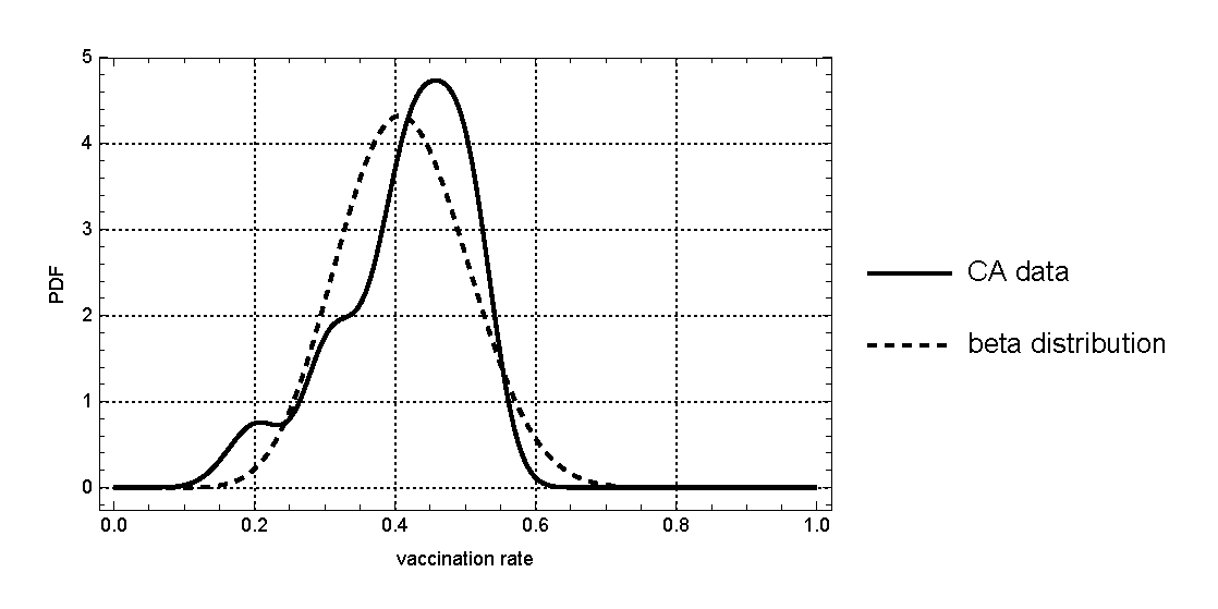
For our comparative analysis, we assume that the county-level vaccination rate is a random variable distributed according to Beta distribution. The Beta distribution gives us the flexibility to easily isolate the effects of changes in variance apart from changes in mean. The distribution is specified with two shape parameters, (\(\rho_{1}, \rho_{2}\)), where the mean of the random variable is \(\frac{\rho_{1}}{\rho_{1} + \rho_{2}}\) and the variance is \(\frac{\rho_{1} \rho_{2}}{(\rho_{1} + \rho_{2})^{2} (\rho_{1} + \rho_{2} + 1)}\) We can solve for the values of \(\rho_{1}\) and \(\rho_{2}\) which give us the distribution having the same mean and variance as the California vaccination rates, \(\hat{\mu}\) and \(\hat{\upsilon}\), by simply setting \(\hat{\mu} = \frac{\rho_{1}}{\rho_{1} + \rho_{2}}\) and \(\hat{\upsilon} = \frac{\rho_{1} \rho_{2}}{(\rho_{1} + \rho_{2})^{2} (\rho_{1} + \rho_{2} + 1)}\), and solving for \(\rho_{1}\) and \(\rho_{2}\). The corresponding values are: \(\rho_{1} = 11.9152\) and \(\rho_{2} = 16.9149\). We will use these values (and the corresponding Beta distribution) as the baseline for our analysis. In Figure 4, we plot the probability density function given the above values for the two shape parameters (dotted curve) as well as the kernel density estimates of the actual California data (solid curve) for visual comparison. Obviously, the Beta density has the same mean and variance as the original California data.
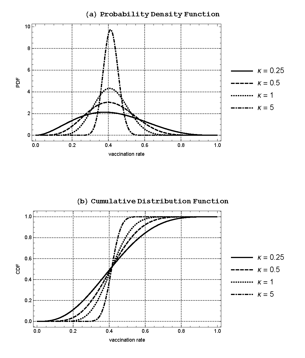
Given the baseline values for \((\rho_{1}, \rho_{2})\), it is straightforward to manipulate the Beta distribution function, changing the variance of the distribution while keeping the mean fixed by scaling the two shape parameters. We define a scale parameter \(\kappa\) such that \(\hat{\rho_{1}} = \kappa \rho_{1}\) and \(\hat{\rho_{2}} = \kappa \rho_{2}\). The mean of the Beta distribution is then independent of \(\kappa\), while the variance is negatively related to \(\kappa\). For our experiments, we consider four different values of \(\kappa\) such that \(\kappa \in \{0.25, 0.5, 1.5\}\). The values of \((\hat{\rho_{1}}, \hat{\rho_{2}})\) as well as the mean and variance of the corresponding Beta distribution are provided for each value of \(\kappa\) in Table 2.
| \(\hat{\rho_{1}}\) | \(\hat{\rho_{2}}\) | \(E[X]\) | \(Var[X]\) | |
|---|---|---|---|---|
| \(\kappa = 0.25\) | 2.9788 | 4.22874 | 0.41329 | 0.0295437 |
| \(\kappa = 0.5\) | 5.9576 | 8.45747 | 0.41329 | 0.0157301 |
| \(\kappa = 1.0\) | 11.9152 | 16.9149 | 0.41329 | 0.00812873 |
| \(\kappa = 5.0\) | 59.576 | 84.5747 | 0.41329 | 0.00167055 |
We show in Figure 5 the probability density functions (PDF) and the cumulative distribution functions (CDF) of the Beta distribution for the chosen values of \(\kappa\), where the variance is greater (smaller) for lower (higher) values of \(\kappa\) while the mean stays fixed at \(\hat{\mu}(=0.41329)\). Note that \(\kappa = 1\) corresponds to the baseline Beta distribution that generates the same mean and variance as the California vaccination data. Using these Beta distributions, we can generate the random variates that will give us the vaccination rates for each region in our computational model. For each season, we take each region within the model and draw a vaccination coverage variable from the Beta distribution. Each region has an independent draw of vaccination coverage. Then we randomly vaccinate each individual agent within each region with a probability equal to the draw for that particular region.
Spatial infection dynamics
Each computational experiment performed for a given set of parameter values consists of multiple seasons, where each season is indexed by \(s\). These seasons are independent in that we assume each season starts with a new strain of virus, which spreads in the population through the contact networks of individual agents as described in Section 3.1.
The underlying mechanism for the infection dynamics is the \(SEIR\) (Susceptible-Exposed-Infectious-Recovered) epidemic process, which is an extended version of the standard \(SIR\) model. In this framework, when a susceptible (unvaccinated) agent comes in contact with an infectious agent, the susceptible agent moves into the exposed state with a fixed probability, \(\omega\). The agent in the exposed state then moves into the infectious state and then to the recovered state after a fixed number of periods. An agent thus recovered stays immune to future infection for the current season. A vaccinated agent immediately moves into the recovered state, becoming immune for the rest of the season.
Specifically, at \(t=0\) of each season we assign the vaccination status – i.e., vaccinated (\(V\)) or unvaccinated (\(NV\)) – to all agents, using the regional vaccination rates as described in Section 3.2. The vaccination status, once specified in \(t=0\), remains fixed for the remainder of the season.
At each time period, \(t \geq 1\), of a given season, \(s\), the state of an agent, \(i\), is defined by his vaccination status, \(v_{i}(s) \in \{V, NV\}\), and his infection status, \(f_{i}^{t}(s)\), where, \(f_{i}^{t}(s)\), can take one of the following four states: 1) susceptible (\(S\)); 2) exposed (\(E\)) – infected but not yet infectious; 3) infected and infectious (\(I\)); 4) recovered and immune (\(R\)). We initiate the contagion dynamic in each season by seeding the population with a small number of infected agents at the beginning of the season. These seed agents, chosen randomly with uniform distribution from the unvaccinated population, have their state set to (\(NV\), \(E\)) at \(t=1\). In all our computational experiments, we set the number of seed agents at 10, sufficiently low to guarantee that the epidemic dynamics are driven by the interactions of agents in the model. All other unvaccinated agents in the population are specified to be susceptible at \(t=1\).
The spread of the disease over time is then captured by how the members of the population, given their vaccination status and infection status in \(t=1\), update their infection state over time, as they interact with one another through their contact networks each period. The interactions with the close contacts take place simultaneously for all agents in the population and we update their infection states simultaneously at the end of each period. Specifically, a susceptible (unvaccinated) agent (i) can get infected through contact with an infectious agent in his network, \(C(i)\). Let \(n_{i}^{t}(s)\) be the number of ‘infectious’ agents in \(C(i)\) in period \(t\) of a given season, \(s\). The transmission of the virus between individuals is probabilistic in that a susceptible agent, when he comes into contact with an infectious agent, gets infected with a fixed probability \(\omega\). Hence, given \(n_{i}^{t}(s)\) infectious agents in \(C(i)\), the likelihood of a susceptible agent i getting infected is \(q(n_{i}^{t}(s))\) where:
| \[ q(n_{i}^{t}(s)) = 1 - (1 - \omega)^{n_{i}^{t}(s)}\] | \[(18)\] |
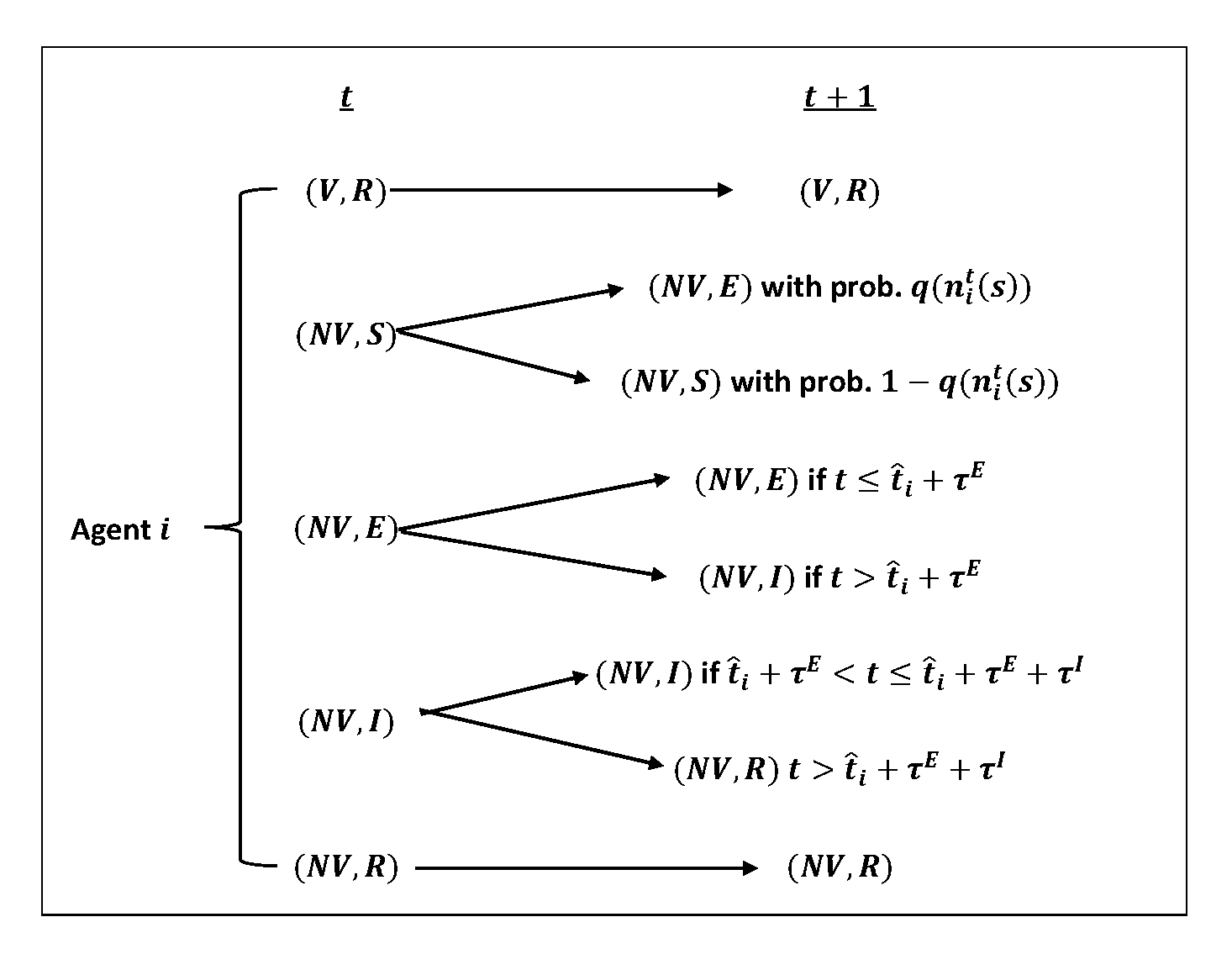
Hence, a susceptible agent \(i\) becomes exposed (\(E\)) in \(t+1\) with probability\(q(n_{i}^{t}(s))\). Denote by \(\hat{t_{i}}(s)\) the first period agent \(i\)’s infection state became \(E\). The state transition rules for an individual agent from \(t\) to \(t+1\) of a typical season may then be summarized as:
- Those agents who were vaccinated in \(t=0\) become immune (\(R\)) to the virus and remain protected for the entire season.
- An unvaccinated agent who is susceptible (\(S\)) gets infected and enters the exposed state (\(E\)) with a probability, \(q(n_{i}^{t}(s))\), where \(n_{i}^{t}(s)\) is the number of agents in \(C(i)\) who are infectious in \(t\). With probability \(1 - q(n_{i}^{t}(s))\), the agent avoids infection and stays susceptible.
- An agent who is infected but not yet infectious (\(E\)) remains in that state for \(\tau^{E}\) periods after the date of infection, \(\hat{t_{i}} (s)\). Once past the \(\tau^{E}\) periods, he becomes infectious (\(I\)) himself.
- An agent who was infected at \(\hat{t_{i}} (s)\) gets infectious (\(I\)) starting \(\hat{t_{i}} (s) + \tau^{E}+1\). The state of \(I\) lasts for \(\tau^{I}\) periods – i.e., from \(\hat{t_{i}} (s) + \tau^{E}+1\) to \(\hat{t_{i}} (s) + \tau^{E}+ \tau^{I}\) – at the end of which the infected agent recovers and becomes immune (\(R\)) to the virus for the remainder of the season.
- A recovered agent remains in that state (\(R\)) for the remainder of the season.
- The seasonal epidemic ends when there is no infected agent in the population – i.e., no one is in the state of (\(NV\), \(E\)) or (\(NV\), \(I\)). This is an absorbing state for the population, since, once it reaches this state, there is no one who can pass on the infection to others either in the current period or in the future periods.
Note that this model produces results as a theoretical exercise and it is not intended to specifically mimic an observed real-world outcome. Thus, we do not “validate” our model in comparison to existing data as is sometimes done with agent-based models. We do perform a wide range of sensitivity analysis across many model parameters as described below. We also emphasize that the underlying distribution used to set the heterogeneous regional vaccination coverage comes from existing data as described above.
Design of Computational Experiments
We simulate a sequence of 100 ‘epidemic seasons’ (replications) for each parameter set considered and report averages and other statistics over these replications. For each season, we exogenously assign each agent in the population a vaccination status in \(t=0\) as described above. This gives us \(v_{i}(s)\) for all \(i \in Z\) in the given season \(s\). All agents who are vaccinated, \(v_{i}(s) = V\), gain immunity such that \(f_{i}^{1}(s) = R\). Those agents who are unvaccinated, \(v_{i}(s) = NV\), become susceptible such that \(f_{i}^{1}(s) = S\). We randomly pick ten (10) of these unvaccinated agents as seed agents. For each seed agent, \(k\), we specify \((v_{k}(s), f_{k}^{1}(s)) = (NV, E)\), setting \(\hat{t_{k}}(s) = 1\) (the date of infection for the seed agent \(k\)).
Given \((v_{i}(s), f_{i}^{1}(s))\) for all \(i \in Z\), we follow the previously specified state transition dynamic from \(t=1\) and on, keeping track of \((v_{i}(s), f_{i}^{t}(s))\) for all agents each period. Figure 6 provides a visualization of the state transition rule for an individual agent from \(t\) to \(t+1\) as described in Section 3.3.
The epidemic continues as long as there are individual agents who are infected. The epidemic ends when no one in the population is in the state of exposed (\(E\)) or infectious (\(I\)) such that the population contains only susceptible (\(S\)) and/or immune (\(R\)) individuals. Denote by \(\hat{T}(s)\) the earliest period that we observe no infected individual in the population. Once the population reaches \(\hat{T}(s)\), there is no possibility of further contagion. A new season, \(s+1\), starts where the population goes through the same sequence of events until it reaches \(\hat{T}(s+1)\).
For each season, the epidemic is the chain of infections by the individuals in the population. We indicate the “size” of an epidemic with the total number of people who were infected over the course of the epidemic. The simulation outputs on the epidemic sizes are collected for all 100 seasons. We analyze how the relevant parameters affect the distribution of these outputs.
Recall that we construct the contact networks of all individuals in a structured way such that each agent has \(\phi\) fraction of his network composed of individuals from his own region and \(1 - \phi\) fraction from outside the region. We carry out a comparative dynamics analysis with respect to the network structure by considering multiple values for \(\phi\), where \(\phi \in \{0.99, 0.975, 0.95, 0.9, 0.8\}\).
For the infection dynamic, we assume that an infected person remains in an exposed (latent) state for two periods (days) before becoming infectious, hence, \(\tau^{E} = 2\). Once an agent becomes infectious, he remains in that state for seven periods (days) before recovering such that\(\tau^{I} = 7\). The probability that the virus is transmitted from an agent to anther agent is set to be \(\omega = 0.02\).
Results
Preliminary results
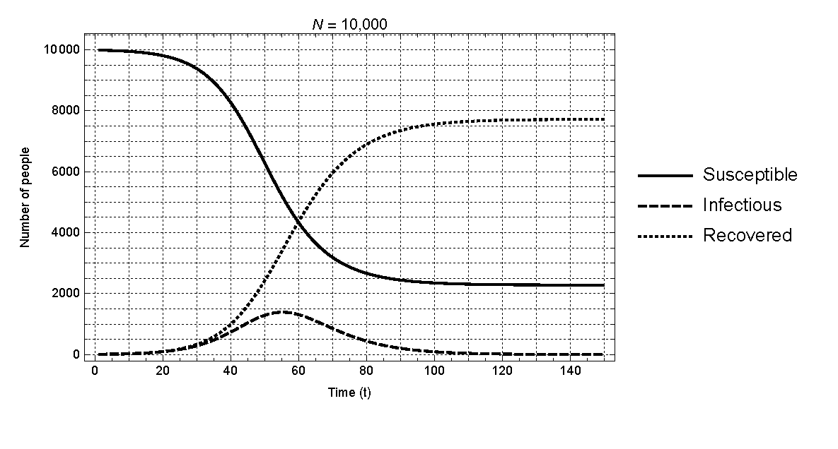
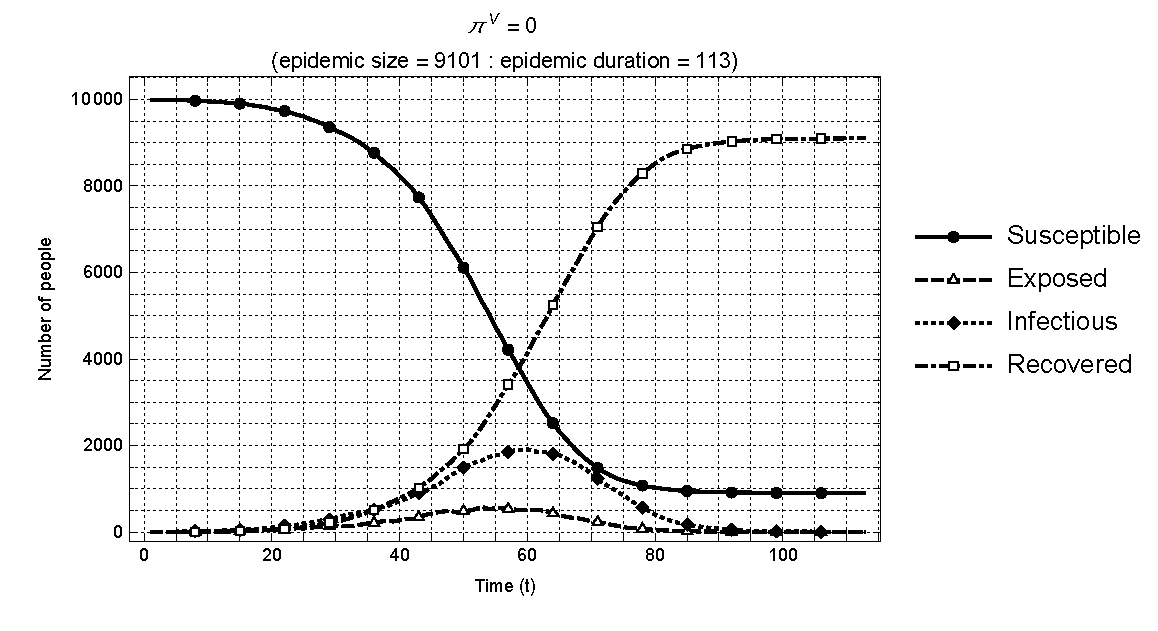
Prior to carrying out the planned experiments, we verify the consistency in the behavior of epidemic dynamics in our agent based model with that of the standard \(SIR\) model. In particular, we track the time series output of the numbers of people in the four states (\(S\),\(E\),\(I\),\(R\)) as the infection spreads in a population. For comparison with the standard \(SIR\) model as described previously, we assume no vaccination in the population for this exercise – i.e., \(\pi_{k}^{v} = 0\) for all \(k\). Figure 7 shows the time paths for susceptible, exposed, infectious, and recovered individuals in a typical season when the population consists of 10,000 individuals. As shown, the results are fully consistent with those capturing the same variables in the standard model as previously shown in Figure 2.
Having checked the consistency of our model with the standard model, we proceed to first consider a simple experiment in which the entire population has the uniform rate of vaccination such that \(\pi_{k}^{v} = \pi^{v} \geq 0\) for all 100 regions. Hence, there are no regional differences in the percentage of individuals who are vaccinated. The main purpose of this experiment is to demonstrate that the base model produces results that are qualitatively consistent with our expectation and to provide a benchmark for our main experiments involving heterogeneous vaccine coverage. It should be noted that the benchmark experiment was first reported in Chang & Tassier (2021). We review it here for the purpose of providing a proper context for our main experiment.
A comprehensive set of values are considered for \(\pi^{v}\) in the benchmark case, where \(\pi^{v} \in \{0, 0.1, 0.2, \dots, 0.9\}\). In t=0 of each season, (\(\pi^{v}\times 10000\)) agents are randomly selected from the population and vaccinated. Of the remaining population of unvaccinated agents, ten are randomly selected as the seed agents and artificially infected in \(t=1\) to start the epidemic process.
The results on the size of the epidemics (averaged over the 100 seasons) are visualized in Figure 8 for all \(\pi^{v} \in \{0, 0.1, 0.2, \dots, 0.9\}\) and \(\phi \in \{0.99,0.975,0.95,0.9,0.8\}\). The impacts of \(\pi^{v}\) and \(\phi\) on global epidemics are captured as: (a) surface plot and (b) contour plot. We make the following observations: 1) The mean size of the epidemics decreases with \(\pi^{v}\) in all five cases; and 2) a decline in the local specificity of the contact networks – i.e., an increase in the share of inter-regional linkages – raises the mean size of the epidemics, when the rate of vaccination is low enough to induce epidemics of significant size. These results are intuitive and as expected: A higher rate of vaccination reduces the size of the epidemics, while more globally connected contact networks tend to further increase the size of the epidemic when the rate of vaccination is relatively low – when the rate of vaccination is high, the sizes of the epidemics are too small for the resulting comparisons to have any statistical significance.6 The central property can then be summarized as: When vaccination rates are uniform across all regions, the average size of an epidemic increases with the share of the inter-regional linkages.
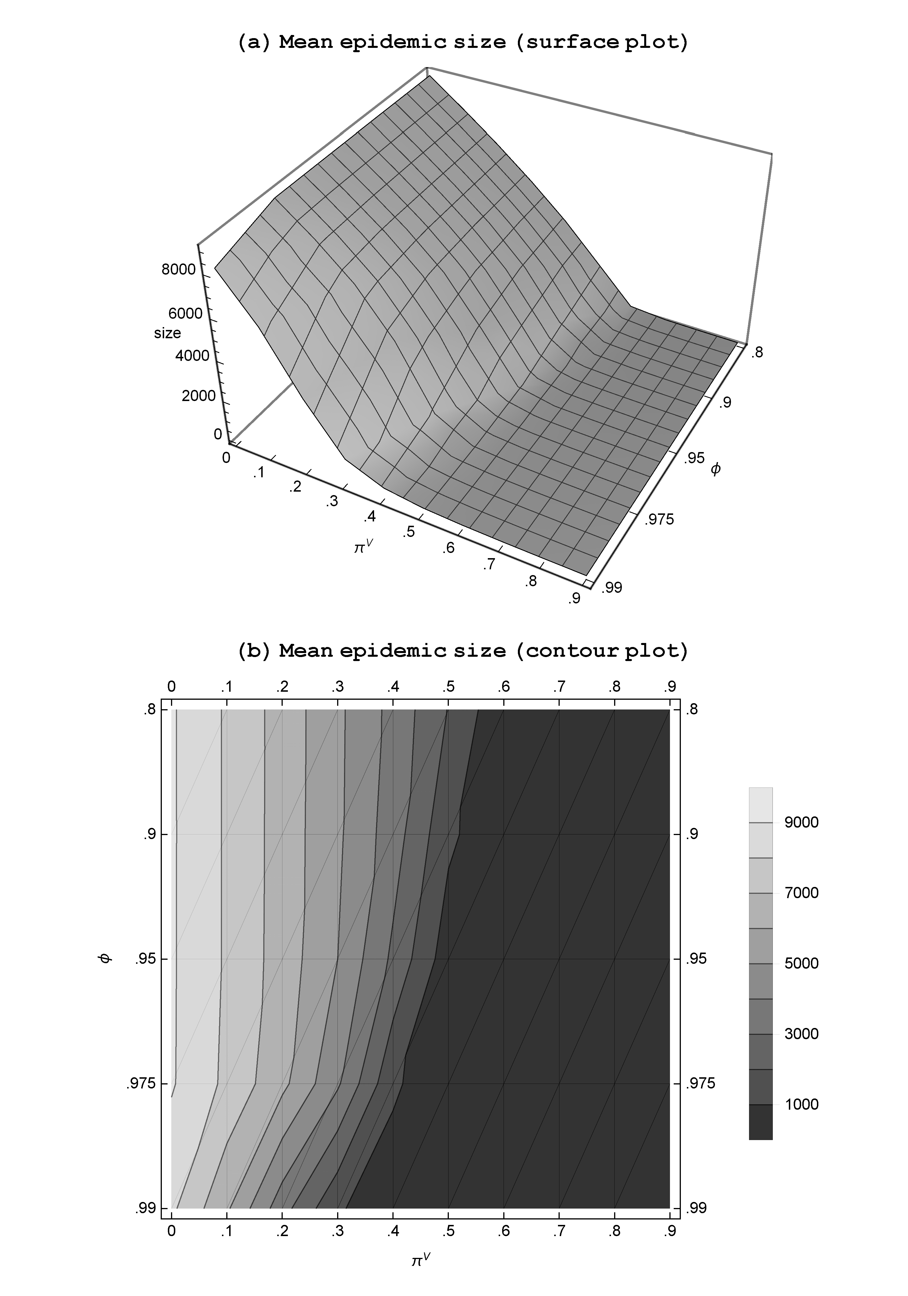
The obvious implication of this property is the increasing importance of vaccinating the population as the contact networks become more inter-regional. If the globalization in the social and economic activities leads to a general increase in the interactions between people of distant regions, an outbreak in one region is likely to have severe and far-reaching consequences; a significant increase in the vaccination effort will be required to keep the epidemic under control. The recent COVID-19 experience offers a clear view of this inherent property where an epidemic involves multiple regions (countries) with cross-regional contacts by the members of the population.
When vaccination rates are spatially heterogeneous
We now introduce spatial heterogeneity in vaccination rates in our model by allowing the regional vaccination rates to vary across regions. This is done by assuming a base distribution for the regional vaccination rates and then specifying the fraction of the vaccinated individuals in each region based on that distribution. The vaccination status of an individual in \(t=0\) can be assigned probabilistically according to the specified rate of his home region. The infection and transmission process follow the dynamic as described in Section 3.3, given the vaccination state of the population.
The first step in the process is to specify the base distribution for the regional vaccination rates. This is done according to the procedures described in Section 3.2.
Size of the global epidemics
We first establish the relationship between the variability in the regional vaccination rates (as captured by \(\kappa\)) and the characteristics of the resulting epidemics. We further examine how this relationship is influenced by the structure of the contact networks, \(\phi\). In characterizing an epidemic, we focus on the mean size of epidemic in a given season, which is simply the number of individuals in the global population who were infected and recovered over the course of the epidemic.
We simulate 100 independent epidemics for each pair of \(\kappa\) and \(\phi\), where \(\kappa \in \{0.25,0.5,1,5\}\) and \(\phi \in \{0.99,0.975,0.95,0.9\}\). The mean and the standard deviation of the epidemic sizes from the 100 independent seasons are reported in Table 3. It is clear that a reduction in the variance of the vaccination rates (higher value of \(\kappa\)) reduces the size of an epidemic, while a higher share of the inter-regional linkages (lower value of \(\phi\)) in individual contact networks raises the size of an epidemic. This result confirms and generalizes the property identified in the case of the two-region model of Chang & Tassier (2021).
| \(\kappa\) | |||||
|---|---|---|---|---|---|
| 0.25 | 0.5 | 1 | 5 | ||
| \(\phi\) | 0.99 | 643.10 (306.76) | 486.69 (211.03) | 398.13 (165.11) | 331.29 (138.57) |
| 0.975 | 1839.64 (686.39) | 1422.86 (559.10) | 1158.13 (542.11) | 877.08 (451.13) | |
| 0.95 | 3207.16 (355.45) | 2960.41 (344.47) | 2686.81 (404.92) | 2561.93 (422.48) | |
| 0.9 | 3606.50 (309.88) | 3459.54 (268.41) | 3335.28 (248.75) | 3241.72 (202.28) | |
Assessing the risk of infection by a susceptible individual
While the "size" of an epidemic gives us the most straightforward indication of the impact vaccination has on the infection dynamic, another impact is measured by the rate of infection, which is defined as the proportion of those at risk – i.e., unvaccinated – who get infected over the course of the epidemic season:
| \[ rate \; of \; infection = \frac{number \; of \; infected \; individuals}{number \; of \; unvaccinated \; individuals}\] | \[(19)\] |
This rate of infection may be viewed as the risk that an agent would face if he remains unvaccinated. This risk, however, may be measured at different levels, depending on which group of the population one is looking at.7 First, it may be measured using global information such as the fraction of infected agents of those unvaccinated in the entire population. We will call this the "global" rate of infection. Second, we may focus on the vaccination and infection data at the regional level – the fraction of infected agents of those unvaccinated in the agent’s home region. We shall call this the "regional" rate of infection. Finally, we can measure the infection risk at the individual agent level – the fraction of infected agents of those unvaccinated in the agent’s specific contact network. This is the "network-specific" rate of infection. Considering the infection risk at these distinct levels is important when we consider the actual decision mechanism that may form the basis for the vaccination rates assumed exogenously in the current model. Although we do not endogenize the vaccination decisions in this paper, we take a preliminary step in this direction by exploring the implications of assessing the risk of infection using these different measures, each of which may play a role in real-life vaccination decisions.
Global rate of infection
The mean and standard deviation of the global rate of infection are reported in Table 4 for all values of \(\kappa\) and \(\phi\). We find that the global risk of infection increases when there is a greater variability in the regional vaccination rates (\(\kappa\) decreases) and a greater share of cross-regional linkages in the contact networks (\(\phi\) decreases).
| \(\kappa\) | |||||
|---|---|---|---|---|---|
| 0.25 | 0.5 | 1 | 5 | ||
| \(\phi\) | 0.99 | 0.109 (0.051) | 0.083 (0.035) | 0.068 (0.028) | 0.056 (0.024) |
| 0.975 | 0.313 (0.113) | 0.242 (0.094) | 0.197 (0.091) | 0.149 (0.076) | |
| 0.95 | 0.544 (0.049) | 0.503 (0.051) | 0.457 (0.065) | 0.436 (0.070) | |
| 0.9 | 0.613 (0.036) | 0.589 (0.034) | 0.568 (0.034) | 0.553 (0.031) | |
Property 1: The global rate of infection is positively related to the variability in the regional vaccination rates and negatively related to the local specificity of the contact networks: (a) The more variable the regional vaccination rates, the higher is the global rate of infection; (b) the larger the share of the cross-regional linkages in the contact networks, the higher is the global rate of infection.
For each pair of values for \(\kappa\) and \(\phi\), we have 100 independent replications (seasons). In Table 5, we provide the correlations between the realized global rates of vaccination and the global rates of infection from those replications for the complete set of values for \(\kappa\) and \(\phi\). In all cases, we see negative and large correlations. The correlation increases in magnitude when the vaccination rates become more variable (\(\kappa\) decreases) and the contact networks more cross-regional (\(\phi\) decreases).
| \(\kappa\) | |||||
|---|---|---|---|---|---|
| 0.25 | 0.5 | 1 | 5 | ||
| \(\phi\) | 0.99 | -0.250947 | -0.238528 | 0.028857 | -0.0852782 |
| 0.975 | -0.419644 | -0.393557 | -0.322155 | -0.289305 | |
| 0.95 | -0.698763 | -0.623428 | -0.530409 | -0.410916 | |
| 0.9 | -0.767432 | -0.729904 | -0.752709 | -0.445848 | |
Regional rate of infection
The next step is to get a finer-grained perspective by zooming in on the relationships between the regional vaccination rates and the regional infection rates. Recall that the population in our model is distributed among 100 regions, each region having 100 agents. For a given season (replication), there are then 100 observations of regional vaccination rates and infection rates. Since we run 100 independent replications, this gives us a total of \(10,000\) (\(=100 \times 100\)) observations of the two rates for any given set of parameter values. A macro-level view of the relationship between vaccination and infection can be obtained by simply plotting these 10,000 observations of the vaccination and infection rates against each other. In Figure 5 we offer for each value of \(\kappa\) a scatter plot of all observed rates of vaccination and infection on the left and the histogram of the infection rates on the right; for all these replications the local specificity of the networks was held fixed at the baseline level of \(\phi = 0.95\).
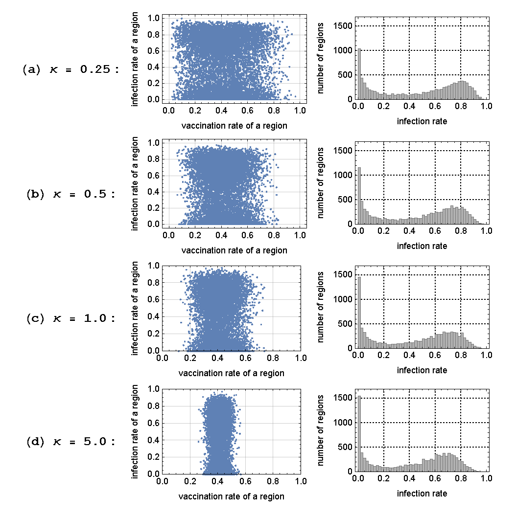
The most striking aspect of these plots is the bimodality in the histograms of the infection rates: there is a cluster of cases near zero infections and another cluster of cases around a positive and substantial rate of infection (\(\approx 0.8\)). The bimodality result implies a rather significant gap in the local infection rates that could exist between neighboring regions – i.e., in some regions, the unvaccinated individuals may be infected at a high rate, while a similar group in their neighboring regions may remain free of the epidemic.
The scatter plots (for all values of \(\kappa\)) also show that there is no significant correlation between the regional vaccination rates and the regional infection rates. Whether or not an unvaccinated agent gets infected depends more on the randomness in the location of the initial source of the outbreak as well as the random realization of the transmission linkages (via contact networks), rather than the vaccination rate of the home region. It should be noted that this absence of correlation is with respect to the regional infection rate, and not the regional epidemic size. The regional epidemic size, which is the absolute number of the infected individuals in the region, is negatively correlated with the regional vaccination rate, as expected, such that those regions with high vaccination rates will experience a smaller number of infected individuals on average. The regional epidemic size, however, is only one measure of the impact that vaccination has on the infection process, as the number of infected individuals is directly influenced by the number of vaccinated individuals; the higher the rate of vaccination, the lower is the number of unvaccinated individuals, which also implies a lower number of infected individuals.
Figure 10 gives us similar relationship between the regional rates of vaccination and infection for various values of \(\phi\), given \(\kappa = 1\). When \(\phi = 0.99\), the regions are relatively segregated. The outbreaks tend to be local and limited to those regions randomly seeded with the initial infection at \(t=0\); many regions remain free of infection. As \(\phi\) is lowered from 0.99 to 0.975, we notice that those regions without the seed infection may experience an outbreak if some of their members are connected to the infected individuals in the seeded regions – we start observing the previously mentioned bimodality in the distribution of infection rates. As \(\phi\) is further lowered, an increasing number of regions experience significant outbreaks – all regions are vulnerable by the time we get to \(\phi = 0.9\). We then observe from Figure 10 the general movement of the points from the cluster representing the low rate of infection to that representing the high rate of infection, as the value of \(\phi\) goes down.
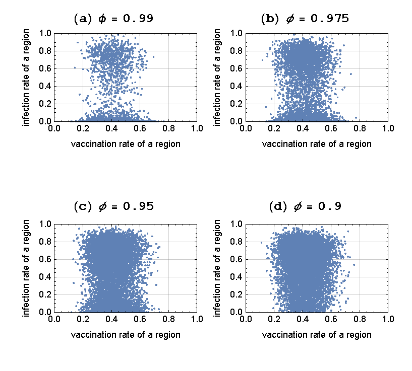
As observed in Figure 9 for various values of \(\kappa\), there is again a lack of correlation between the regional rates of vaccination and the regional rates of infection. This property is shown to hold more generally in Table 6: We detect no significant correlation between the two rates for all pairs of \(\kappa\) and \(\phi\) considered in this paper.
| \(\kappa\) | |||||
|---|---|---|---|---|---|
| 0.25 | 0.5 | 1 | 5 | ||
| \(\phi\) | 0.99 | -0.0150282 | -0.0297019 | -0.0100962 | 0.0185661 |
| 0.975 | -0.066773 | -0.0276384 | -0.0103178 | -0.00127095 | |
| 0.95 | -0.076256 | -0.0691128 | -0.0376693 | -0.029411 | |
| 0.9 | -0.0498369 | -0.0491849 | -0.0534663 | -0.0260599 | |
Property 2: There is no relationship between the regional rate of vaccination and the regional rate of infection.
Network-specific rate of infection
The last measure of the infection risk is that which is assessed at the level of the individual agent’s contact network. We saw from the previous section that the regional rate of vaccination gives us no indication of the risk of infection within that region. The question we ask now is whether the rate of vaccination within an individual agent’s contact network is an indicator of the risk of infection for the agent.
For each season, we have a population of 10,000 agents. Given the vaccination rates specified for the season, some of these agents are vaccinated, while others are unvaccinated and are susceptible to infection. Because vaccination is perfect in our model, the risk of infection is a relevant issue only for the unvaccinated population. As such, our focus will be strictly on the unvaccinated agents in the population for this measure of the infection risk. For each unvaccinated agent, \(k\), such that \(v_{k}(s) = NV\), let us examine their contact networks, \(C(k)\), and count the number of contacts who are also unvaccinated. Define \(G(k)\) as the set of unvaccinated agents in the population who have exactly \(K\) number of unvaccinated contacts in their networks. Further define \(g(K) \subseteq G(K)\) as the set of those in \(G(k)\) who ended up being infected during the season. The likelihood of an unvaccinated agent with \(K\) unvaccinated contacts getting infected may then be expressed as: \(\gamma (K) \equiv \frac{\lvert g(K) \rvert}{\lvert G(K) \rvert}\). \(\gamma (K)\) is, hence, the fraction of the susceptible agents with \(K\) unvaccinated contacts who are eventually infected during the season. It is a measure of how likely it is for an unvaccinated agent having \(K\) unvaccinated contacts to become infected. In Figure 11 we plot \(\gamma (K)\) for the baseline case of \(\phi = 0.95\).
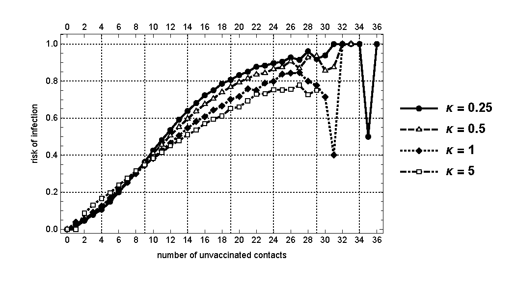
The main insight here is that for all values of \(K\) such that there are sufficient numbers of unvaccinated agents, \(\gamma (k)\) is positively related to \(K\): Those unvaccinated individuals with a greater number of unvaccinated contacts are more likely to be infected. Furthermore, the network-specific risk of infection tends to be higher for lower values of \(\kappa\). Note that the plots are quite noisy for high values of \(K\) (above 27). This is due to the fact that there are few contact networks with such high numbers of unvaccinated contacts; hence the results are not statistically significant for this range of values of \(K\).
In Figure 12, we plot \(\gamma (K)\) for \(\phi \in \{0.99,0.975,0.9\}\) and confirm that the above result is robust to varying the structure of the networks.
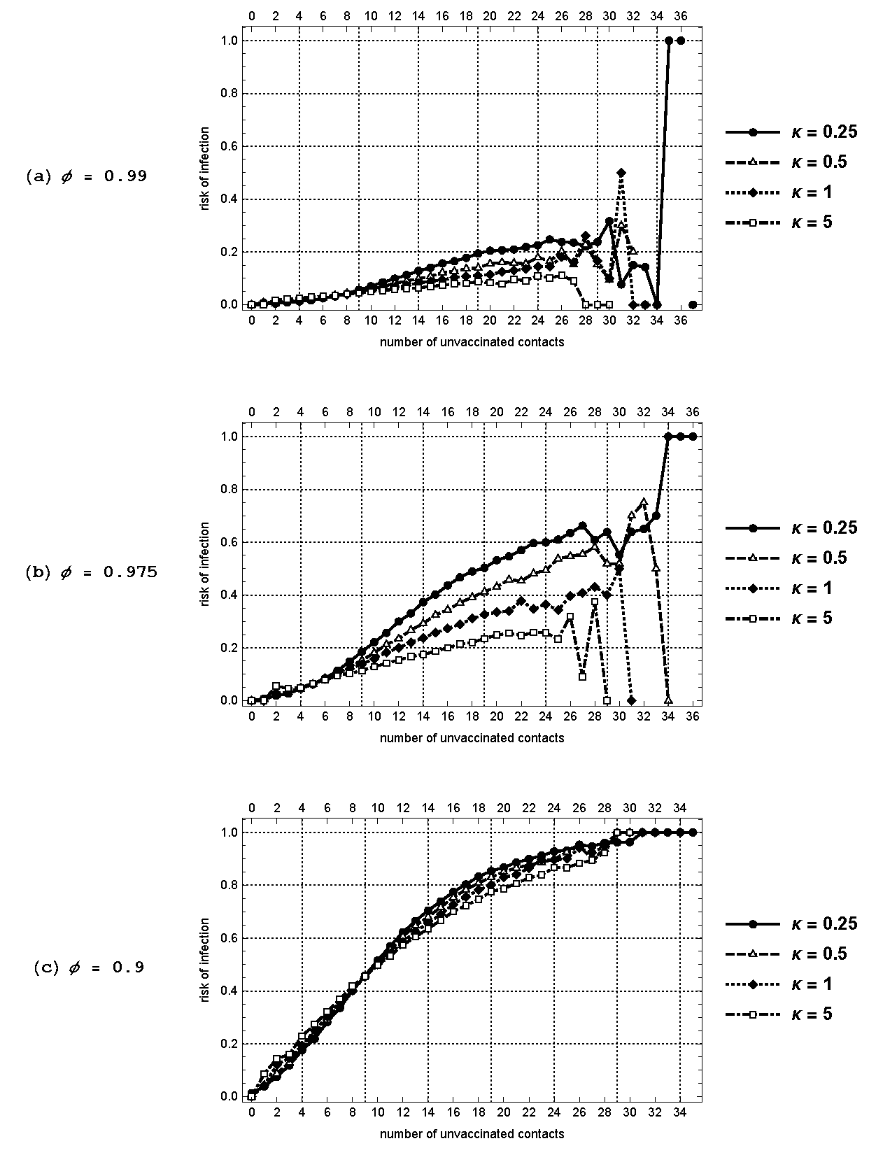
Property 3: Individuals with a larger number of unvaccinated contacts are more likely to be infected and the risk of infection is higher when the vaccination rates are more variable across regions.
Properties 1-3, taken together, suggest non-monotonicity in the relationship between local vaccine information and rate of infection at varying levels of aggregation. Rate of infection is highly correlated with the global rate of unvaccinated individuals and the number of direct contacts who are unvaccinated. However, the rate of vaccination in one’s own region is not significantly correlated with rate of infection. This gives clues as to what information would be useful to agents’ decision making with respect to vaccination. Very precise contact level information or global vaccination information is likely to lead to an accurate assessment of infection risk. However, intermediate level information about one’s region does not in our model.
Finally, our result on regional rate of infection (Property 2) is of particular interest when we consider its implications in the context of the on-going COVID-19 pandemic. As is observed on a daily basis, the national media in various countries often focus on reporting their own internal rates of vaccination and infection without a comparable coverage over the state of pandemic in neighboring countries and the potential for cross-border interactions. The implicit signal here is that the causal relationship exists only between the internal rate of vaccination and internal rate of infection. Clearly, our findings suggest that the vaccine policy based on this belief is likely to be inadequate. The vaccine strategy at the national level requires a coordination with those of other countries through extensive sharing and dissemination of information.
Conclusion
MEDITATION XVII, Devotions upon Emergent Occasions, John Donne
In this paper we investigate the impact that heterogeneity in regional vaccine coverage have on global epidemics. Addressing this issue requires a model with two essential features: 1) population divided among multiple regions with heterogeneous vaccine coverage; 2) interconnected contact networks that allow individuals to have both intra-regional interactions and inter-regional interactions. These two features call for an approach which has the capacity to go beyond what is allowed by the standard compartmental models. In order to add these essential features without losing analytical tractability, we develop an agent-based computational model of infectious disease with spatial heterogeneity in vaccine coverage. The model isolates the effects of heterogeneity by holding overall vaccination coverage rates constant. We find that spatial heterogeneity by itself has significant implications for understanding epidemic dynamics. Specifically, an increase in spatial heterogeneity leads to larger epidemics on average. This effect is magnified when more interregional connections exist in the contact structure of the model.
In the model we find non-monotonic relationships in infection risk of unvaccinated individuals. Infection risk of an unvaccinated individual decreases in both the global rate of vaccinations and the rate of vaccination of the individual’s specific contacts. But, surprisingly, we find that the vaccination rate in an individual’s home region does not have a significant impact on an individual’s infection risk in our model. This has significant implications for an individual’s vaccine choices. Global and local (network specific) vaccination rates are highly correlated with infection risk and thus should be prioritized as information sources for an agent’s rational decision making. Using regional (e.g., school or neighborhood) specific information is likely to lead to non-optimal decisions unless those regional vaccination rates are highly correlated to global vaccine coverage (as in the uniform vaccine coverage example) or if the vaccination rates of individual level contacts match regional rates.
The cross-regional/cross-border contact networks in our model may be viewed as arising endogenously from the more general and larger system of complex and interconnected networks that characterize the global transport network, supply chains, and the financial systems. While acknowledging the substantial social and economic benefits from the rapid diffusion of knowledge and the flexible migration of resources over these underlying networks, we must also recognize the potential systemic risks in the form of catastrophic damages to ecological, environmental, and public health state of the population at the global scale. The agent-based computational approach as proposed in this paper represents a step toward understanding the risks inherent in such complex interconnected systems and developing an effective coordination mechanism for reducing the potential damage.
Appendix A
| Overview(O) | 1. Purpose and Patterns | To trace the infection status of the multi-regional population given spatially heterogeneous vaccination rates |
| 2. Entities, State Variables and Scales | A population of 10,000 autonomous agents, spread among 100 separate regions; | |
| State variables include the vaccination state and the infection state of the individual agents. | ||
| 3. Process Overview & Scheduling | A sequence of 100 epidemic seasons; | |
| Each season starts with artificial introduction of infectious virus into a population of agents; | ||
| The infection spreads through SEIR process; | ||
| A season ends only when there is no infected individual in the population; | ||
| The total number of people who were infected is recorded for each season. | ||
| Design(D) | 4. Design Concepts | The individual agents are connected through their contact networks, where each agent’s contact network contains 20 other agents; |
| The regionality of the population depends on the proportion of the individuals in an agent’s contact network who are from his/her own region. | ||
| Details(D) | 5. Initialization | Vaccination rates in each season are exogenous; |
| Each region is given a mean vaccination rate which is a draw from a beta distribution based on the County-level flu vaccination claims rates for California from 2016-2017 (the data in the Appendix B); | ||
| In each season, the infection process starts with 10 seed agents who get artificially infected; | ||
| The probability that the virus is transmitted from one agent to another is set to be 0.02. | ||
| 6. Input Data | Beta distribution fitted to the county-level flu vaccination claims rates for California from 2016-2017 (see Appendix B). | |
| 7. Submodels | Contact networks; | |
| \(SEIR\) process of infection spread. |
Appendix B
- Beneficiaries: The total number of Medicare fee-for-service beneficiaries for the county
- Vaccination Claims Rate: The number of flu vaccine claims relative to the number of beneficiaries
- Source: https://www.hhs.gov/nvpo/about/resources/interactive-mapping-tool-tracking-flu-vaccinations/index.html (last accessed: 1/10/2018)
| County | Beneficiaries | Rate | County | Beneficiaries | Rate |
|---|---|---|---|---|---|
| Alameda | 88,457 | 46.63 | Orange | 173,864 | 49.71 |
| Alpine | 187 | 20.86 | Placer | 31,501 | 52.95 |
| Amador | 7,096 | 49.86 | Plumas | 4,288 | 21.60 |
| Butte | 40,306 | 40.34 | Riverside | 102,217 | 40.94 |
| Calaveras | 9,211 | 40.50 | Sacramento | 81,305 | 47.16 |
| Colusa | 2,696 | 40.99 | San Benito | 5,860 | 50.17 |
| Contra Costa | 66,924 | 48.12 | San Bernardino | 72,573 | 32.36 |
| Del Norte | 4,685 | 38.14 | San Diego | 179,490 | 43.49 |
| El Dorado | 21,179 | 49.45 | San Francisco | 59,899 | 44.32 |
| Fresno | 67,823 | 46.50 | San Joaquin | 47,402 | 45.23 |
| Glenn | 4,584 | 35.93 | San Luis Obispo | 42,374 | 49.79 |
| Humboldt | 22,099 | 40.52 | San Mateo | 46,165 | 52.17 |
| Imperial | 20,948 | 33.53 | Santa Barbara | 49,909 | 49.25 |
| Inyo | 3,824 | 43.51 | Santa Clara | 100,846 | 53.08 |
| Kern | 52,954 | 37.75 | Santa Cruz | 34,663 | 51.29 |
| Kings | 11,225 | 36.97 | Shasta | 39,276 | 43.04 |
| Lake | 13,613 | 28.54 | Sierra | 701 | 20.11 |
| Lassen | 4,270 | 30.47 | Siskiyou | 10,182 | 30.96 |
| Los Angeles | 501,496 | 41.86 | Solano | 30,236 | 37.76 |
| Madera | 12,200 | 39.79 | Sonoma | 43,086 | 48.11 |
| Marin | 25,920 | 51.93 | Stanislaus | 34,454 | 44.36 |
| Mariposa | 3,546 | 31.02 | Sutter | 13,418 | 51.33 |
| Mendocino | 17,039 | 27.97 | Tehama | 10,667 | 42.22 |
| Merced | 25,393 | 42.72 | Trinity | 2,880 | 30.24 |
| Modoc | 1,856 | 16.86 | Tulare | 41,070 | 43.65 |
| Mono | 1,210 | 31.82 | Tuolumne | 12,202 | 46.75 |
| Monterey | 47,314 | 45.13 | Ventura | 75,213 | 48.11 |
| Napa | 14,057 | 45.52 | Yolo | 12,617 | 52.58 |
| Nevada | 19,143 | 49.46 | Yuba | 9,030 | 41.66 |
Notes
Although not reported in this paper, these results are confirmed for the comparable county-level data from three other representative states as well as the zip code-level data from a selected group of metropolitan cities, hence, demonstrating their robustness across different scales of spatial interactivity.↩︎
For some recent analytical attempts in this direction, see Chen et al. (2014) and Brugnano et al. (2021).↩︎
This model adds an extra state of \(E\) (exposed) to the original \(SIR\) model. An individual in the exposed state is infected but not yet infectious. This is in contrast to an individual in the infectious state (\(I\)) who is infected and also fully infectious.↩︎
The source code for the main experiments reported here was written in Wolfram Mathematica Version 10.4. The original source codes in Mathematica notebook format (.nb) as well as in PDF format are available at: https://myongchang.github.io/research/SourceCodes.html.↩︎
Abbe (2018) provides a survey of recent developments in mathematical models of networks that enable detection of such inter-linked communities. Our model of multi-regional contact networks falls in the category of “stochastic block models” in this literature.↩︎
it is not until \(\pi^{v}\) is sufficiently low that the typical epidemic takes off and proceeds in a manner governed by the complexities of the contact network structure.↩︎
The empirical relevance of the spatial resolution is suggested by a recent study, Baltrusaitis et al. (2018), which examines the impact of the spatial resolution on the correlations between different influenza surveillance systems. Comparing the data at the national, northeast regional, Massachusetts, and the greater Boston levels, they find that an increase in the spatial resolution tends to decrease the correlation values between the different systems.↩︎
References
ABBE, E. (2018). Community detection and stochastic block models: Recent developments. Journal of Machine Learning Research, 18, 1–86.
ASCHWANDEN, C. (2021). Five Reasons Why COVID Herd Immunity Is Probably Impossible. Nature. Available at: https://www.nature.com/articles/d41586-021-00728-2 [doi:10.1038/d41586-021-00728-2]
ATWELL, J. E., van Otterloo, J., Zipprich, J., Winter, K., Harriman, K., Salmon, D. A., Halsey, N. A., & Omer, S. B. (2013). Nonmedical vaccine exemptions and pertussis in California, 2010. Pediatrics, 132(4), 624–630. [doi:10.1542/peds.2013-0878]
BALTRUSAITIS, K., Brownstein, J., Scarpino, S., Bakota, E., Crawley, A., Conidi, G., Gunn, J., Gray, J., Zink, A., & Santillana, M. (2018). Comparison of crowd-Sourced, electronic health records based, and traditional health-Care based influenza-Tracking systems at multiple spatial resolutions in the United States of America. BMC Infectious Diseases, 18, 403. [doi:10.1186/s12879-018-3322-3]
BANSAL, S., Pourbohloul, B., & Meyers, L. A. (2006). A comparative analysis of influenza vaccination programs. PLoS Medicine, 3(10), e387. [doi:10.1371/journal.pmed.0030387]
BARRAT, A., Berthelemy, M., & Vespignani, A. (2010). Dynamical Processes on Complex Network. Cambridge: Cambridge University Press.
BIRNBAUM, M. S., Jacobs, E. T., Ralston-King, J., & Ernst, K. C. (2013). Correlates of high vaccination exemption rates among kindergartens. Vaccine, 31(5), 750–756. [doi:10.1016/j.vaccine.2012.11.092]
BRUGNANO, L., Iavernaro, F., & Zanzottera, P. (2021). A multiregional extension of the SIR model, with application to the COVID-19 spread in Italy. Mathematical Methods in the Applied Sciences, 44, 4414–4427. [doi:10.1002/mma.7039]
BUTTENHEIM, A., Jones, M., & Baras, Y. (2012). Exposure of California kindergartners to students with personal belief exemptions from mandatory school entry vaccinations. American Journal of Public Health, 102(8), e59–e67. [doi:10.2105/ajph.2012.300821]
CARREL, M., & Bitterman, P. (2015). Personal belief exemptions to vaccination in California: A spatial analysis. Pediatrics, 135(1), 80–88. [doi:10.1542/peds.2015-0831]
CDC. (2018). 1995 Through 2017 Childhood Measles, Mumps, and Rubella (MMR) Vaccination Coverage Trend Report. Available at: https://www.cdc.gov/vaccines/imz-managers/coverage/childvaxview/data-reports/mmr/trend/
CDC. (2023). Measles Cases and Outbreaks. Available at: https://www.cdc.gov/measles/cases-outbreaks.html
CHANG, M.-H., & Tassier, T. (2021). Spatially heterogeneous vaccine coverage and externalities in a computational model of epidemics. Computational Economics, 58, 27–55. [doi:10.1007/s10614-019-09918-7]
CHEN, Y., Yan, M., & Xiang, Z. (2014). Transmission dynamics of a two-City SIR epidemic model with transport-Related infections. Journal of Applied Mathematics, 2014, 1–12. [doi:10.1155/2014/764278]
DEL Valle, S. Y., Mniszewski, S. M., & Hyman, J. M. (2013). Modeling the impact of behavior changes on the spread of pandemic influenza. In P. Manfredi & A. D’Onofrio (Eds.), Modeling the Interplay Between Human Behavior and the Spread of Infectious Diseases. Springer. [doi:10.1007/978-1-4614-5474-8_4]
EPSTEIN, J. M. (2009). Modelling to contain epidemics. Nature, 460(6), 687.
EUBANK, S., Guclu, H., Kumar, V. S. A., Marathe, M. V., Srinivasan, A., Toroczkai, Z., & Wang, N. (2004). Modelling disease outbreaks in realistic urban social networks. Nature, 429, 180–184. [doi:10.1038/nature02541]
FEIKIN, D. R., Lezotte, D. C., Hamman, R. F., Salmon, D. A., Chen, R. T., & Hoffman, R. E. (2000). Individual and community risks of measles and pertussis associated with personal exemptions to immunization. Journal of the American Medical Association, 284(24), 3145–3150. [doi:10.1001/jama.284.24.3145]
GERMANN, T., Kadau, K., Longini, I. M., & Macken, C. A. (2006). Mitigation strategies for pandemic influenza in the United States. Proceedings of the National Academy of Sciences, 103(15), 5935–5940. [doi:10.1073/pnas.0601266103]
GERSOVITZ, M. (2013). Mathematical epidemiology and welfare economics. In P. Manfredi & A. D’Onofrio (Eds.), Modeling the Interplay Between Human Behavior and the Spread of Infectious Diseases. Springer. [doi:10.1007/978-1-4614-5474-8_12]
GRIMM, V., Berger, U., Bastiansen, F., Eliassen, S., Ginot, V., Giske, J., Goss-Custard, J., Grand, T., Heinz, S. K., Huse, G., Huth, A., Jepsen, J. U., Jørgensen, C., Mooij, W. M., Müller, B., Pe’er, G., Piou, C., Railsback, S. F., Robbins, A. M., … DeAngelis, D. L. (2006). A standard protocol for describing individual-based and agent-based models. Ecological Modelling, 198(1–2), 115–126. [doi:10.1016/j.ecolmodel.2006.04.023]
GRIMM, V., Berger, U., DeAngelis, D. L., Polhill, J. G., Giske, J., & Railsback, S. F. (2010). The ODD protocol: A review and first update. Ecological Modelling, 221(23), 2760–2768. [doi:10.1016/j.ecolmodel.2010.08.019]
GRIMM, V., Railsback, S. F., Vincenot, C. E., Berger, U., Gallagher, C., DeAngelis, D. L., Edmonds, B., Ge, J., Giske, J., Groeneveld, J., Johnston, A. S. A., Milles, A., Nabe-Nielsen, J., Polhill, J. G., Radchuk, V., Rohwäder, M. S., Stillman, R. A., Thiele, J. C., & Ayllón, D. (2020). The ODD protocol for describing agent-Based and other simulation models: A second update to improve clarity, replication, and structural realism. Journal of Artificial Societies and Social Simulation, 23(2), 7. [doi:10.18564/jasss.4259]
GUST, D. A., Strine, T. W., Maurice, E., Smith, P., Yusuf, J., Wilkinson, M., Battaglia, M., Wright, R., & Schwartz, B. (2004). Underimmunization among children: Effects of vaccine safety concerns on immunization status. Pediatrics, 114(1), e16–e22. [doi:10.1542/peds.114.1.e16]
INGRAHAM, C. (2015). The Devastating Impact of Vaccine Deniers, in One Measles Chart. Washington Post. Available at: https://www.washingtonpost.com/news/wonk/wp/2015/01/22/the-devastating-impact-of-vaccine-deniers-in-one-measles-chart/
LIEU, T. A., Ray, G. T., Klein, N. P., Chung, C., & Kulldorff, M. (2015). Geographic clusters in underimmunization and vaccine refusal. Pediatrics, 135(2), 280–289. [doi:10.1542/peds.2014-2715]
MAY, T., & Silverman, R. D. (2003). Clustering of exemptions as a collective action threat to herd immunity. Vaccine, 21(11–12), 1048–1051. [doi:10.1016/s0264-410x(02)00627-8]
MCNUTT, L.-A., Desemone, C., DeNicola, E., El Chebib, H., Nadeau, J. A., Bednarczyk, R. A., & Shaw, J. (2016). Affluence as a predictor of vaccine refusal and underimmunization in California private kindergartens. Vaccine, 34(14), 1733–1738. [doi:10.1016/j.vaccine.2015.11.063]
OSTER, E., & Kocks, G. (2018). After a Debacle, How California Became a Role Model on Measles. New York Times. Available at: https://www.nytimes.com/2018/01/16/upshot/measles-vaccination-california-students.html
POLAND, G. A., & Jacobson, R. M. (2001). Understanding those who do not understand: A brief review of the anti-vaccine movement. Vaccine, 19(17–19), 2440–2445. [doi:10.1016/s0264-410x(00)00469-2]
SEITHER, R., Calhoun, K., Yusuf, O. B., Dramann, D., Mugerwa-Kasujja, A., Knighton, C. L., & Black, C. L. (2023). Vaccination Coverage With Selected Vaccines and Exemption Rates Among Children in Kindergarten - United States, 2021–22 School Year. Morbidity and Mortality Weekly Report (MMWR). Available at: https://www.cdc.gov/mmwr/volumes/72/wr/mm7202a2.htm?s_cid=mm7202a2_w [doi:10.15585/mmwr.mm7202a2]
SMITH, D. J., Forrest, S., Ackley, D. H., & Perelson, A. S. (1999). Variable efficacy of repeated annual influenza vaccination. Proceedings of the National Academy of Sciences, 96(24), 140001–140006. [doi:10.1073/pnas.96.24.14001]
STROUD, P., Del Valle, S., Sydoriak, S., Riese, J., & Mniszewski, S. (2007). Spatial dynamics of pandemic influenza in a massive artificial society. Journal of Artificial Societies and Social Simulation, 10(4), 9.
SUGARMAN, D. E., Barskey, A. E., Delea, M. G., Ortega-Sanchez, I. R., Bi, D., Ralston, K. J., Rota, P. A., Waters-Montijo, K., & Lebaron, C. W. (2010). Measles outbreak in a highly vaccinated population, san diego, 2008: Role of the intentionally undervaccinated. Pediatrics, 125(4), 747–755.
TASSIER, T., Polgreen, P., & Segre, A. (2017). Network position and healthcare worker infections. Journal of Economic Interaction and Coordination, 12, 277–307. [doi:10.1007/s11403-015-0166-4]
TIZZONI, M., Bajardi, P., Poletto, C., Ramasco, J. J., Balcan, D., Gonçalves, B., Perra, N., Colizza, V., & Vespignani, A. (2012). Real-time numerical forecast of global epidemic spreading: Case study of 2009 A/H1N1pdm. BMC Medicine, 165, 2012. [doi:10.1186/1741-7015-10-165]
VARDAVAS, R., & Marcum, C. S. (2013). Modelling influenza vaccination behavior via inductive reasoning games. In P. Manfredi & A. D’Onofrio (Eds.), Modeling the Interplay Between Human Behavior and the Spread of Infectious Diseases. Springer. [doi:10.1007/978-1-4614-5474-8_13]
WATTS, D. J., & Strogatz, S. H. (1998). Collectives dynamics of small-world networks. Nature, 393, 440–442. [doi:10.1038/30918]