DARTS: Evolving Resilience of the Global Food System to Production and Trade Shocks

,
and
aWageningen Plant Research, Wageningen University and Research, Wageningen, The Netherlands; aWageningen Plant Research, Wageningen University and Research, Wageningen, The Netherlands; bNetherlands Institute of Ecology (NIOO), Wageningen, The Netherlands
Journal of Artificial
Societies and Social Simulation 27 (2) 1![]()
<https://www.jasss.org/27/2/1.html>
DOI: 10.18564/jasss.5307
Received: 04-Aug-2022 Accepted: 21-Jan-2024 Published: 31-Mar-2024
Abstract
This paper presents a new agent-based modelling (ABM) framework to investigate the resilience of food systems against a variety of shocks. We modelled food security as an emergent property from a network of agents that produce, trade and consume food. The network consists of different regions (mimicking the different hemispheres, an equatorial region and a city state with corresponding growing seasons). Each region in turn consists of a rural and urban area. Rural consumers have access to only regionally produced goods, whereas urban consumers can access both intra- and inter-region trade. We studied food security in a hierarchy of 4 archetypical food systems (or ‘Worlds’) evolving from a simple food system in which regions are not urbanised and there is no trade between regions to a globalised World, with a fully connected food system, which is highly urbanised (including a city state with little national food production) and highly interconnected. We investigated the baseline performance of these food systems (no shocks) and the effect of an export ban of one region on food security. We showed first and second-order effects of such a shock in the short- and medium-term, and how these effects differ across food systems. We found that international trade increases food security in the baseline and shock scenario, but also that it can introduce the potential for poor populations to suffer from food system shocks of distant origins. Future work will extend the set of investigated shocks to provide a broader understanding of food systems resilience, possibly in more realistic scenarios.Introduction
Over the past two millennia, food systems have followed three global trends that are visible almost everywhere in the world; globalisation (Ortiz-Ospina et al. 2018), urbanisation (Ritchie & Rosen 2018) and productivity increases (Roser 2013). These developments, together with a substantial increase in wealth across the Western World and (to a lesser degree) the global South (Roser 2013) have caused high levels of food security for the majority of the World population, combined with persistent food insecurity for a substantial minority (Collier 2007). Recent crises (2007-2008 World food price crisis, COVID-19, the Ukrainian war) have shown that food security can be substantially affected by adverse events. Where historically speaking, food security crises were caused by local events (droughts, floods, political unrest), recent crises have generally been caused by a diverse range of global causes. Globalisation has fundamentally changed the network structure of the food system, which in turn, has had a multitude of effects on food security, such as changes in dietary patterns and product convergence and standardisation. With regards to food production and distribution, we can distinguish three major effects of globalisation, two positive (see chapter 2 in Anderson 2016) and one negative:
- Efficiency: many populations now source their food globally. This has two advantages: first, when depending on local production only, food can only directly be sourced during harvest seasons and has to be stocked for the rest of the year. When food from other harvest seasons around the World becomes available, the reliance on food stocks decreases, which thus improves efficiency. Second, each region can now specialise on food it can most optimally produce, which increases the efficiency of world food production generally and reduces costs and prices.
- Risk diversification: since food production is spread across the globe, localised shocks only affect populations that exclusively source food locally. Other populations simply switch to another geographical location to source the same food item, or replace consumption with a comparable food item.
- Unequal risk distribution: food system integration also causes ripple effects of shocks. The global food price crisis of 2007-2008 is a prime example, where a combination of factors (disappointing harvests in Australia and India, increases in oil prices causing increases in fertiliser prices, replacement by biofuel) and hoarding (Conceição & Mendoza 2009, see Dawe 2012 and Slayton 2009 for a detailed discussion on the food price crisis in the rice market) caused food commodity prices to rise dramatically. This in turn had the effect of some large exporting nations to restrict exports, which drove prices up further (Headey 2011). The result was decreased food security for populations, who on the one hand did not have sufficient access to locally produced food and were too poor to afford international prices.
Another important development that has evolved in parallel with globalisation is urbanisation. By 2050 it is projected that more than two thirds of the world population will be living in cities (Ritchie & Rosen 2018). Urbanisation intersects with food security especially in Low- and Middle-Income Countries (LMIC). In many cases, urban populations depend on international markets for food commodities, whereas rural populations depend on locally produced food (Berazneva & Lee 2013). Here, the role of smallholder farmers is especially important, since they constitute a significant portion of both the food producers and the food consumers of the rural poor. Urbanisation therefore exposes the rural poor and urban poor to different risk categories. Whereas the urban poor suffer from unequal risk distribution, since dependence on international markets combined with their weak financial position makes them vulnerable to international price shocks, the rural poor are very vulnerable to local (production) shocks.
Both globalisation and urbanisation have been made possible by a dramatic increase in agricultural yield, caused by the development of high-yielding crops and artificial fertilisers and pesticides to optimise yield (Jain 2010). However, this development has been unevenly distributed across the World. Whereas farming in the developed world has been fully ‘industrialised’, many smallholders in LMICs often make limited use of these techniques.
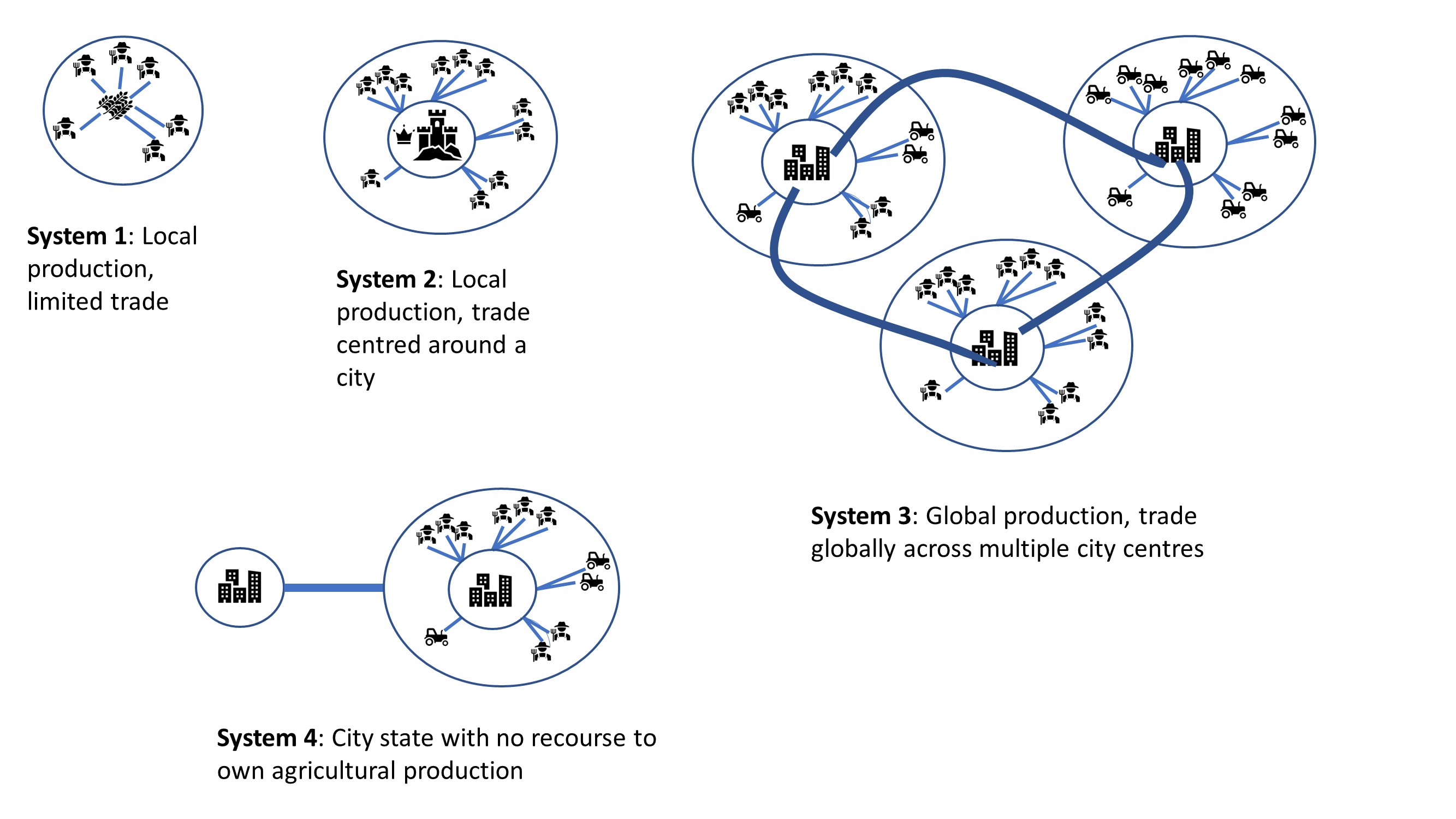
The causal relationship between increases in food production, globalisation of trade and urbanisation are still under debate. However, these factors do suggest a pattern of progression through four food system archetypes, which roughly mimic the development of real food systems in history (Tauger 2010) and are shown in Figure 1. System 1 represents the most localised food system where food production supports subsistence, but with little surplus for trade. System 2 shows the first steps towards larger settlements (urbanisation) where food surpluses lead to specialisation and increased social hierarchies, although the direction of causality between food surpluses on the one hand and specialisation and social hierarchies on the other remains unclear. Trade within system 2 is substantial, whereas trade between different instances of system 2 (e.g., between ancient Rome and ancient China) is limited to non-perishables and non-food commodities. System 3 is characterised by a higher degree of urbanisation, the introduction of industrial agriculture and the widespread trade of commodities and perishables between regions/countries. We have deliberately chosen to represent regions in this system as cities and their (agricultural) hinterland. These regions can be thought of as abstractions of regions, countries and even continents. System 4 represents the extreme of this food system development pattern, in which one region (e.g., a city state such as Singapore) has only very limited local food production and is completely dependent on global markets. It should be noted that food systems can develop further towards even stronger integration (following the narrative described above) or towards disintegration or deglobalisation, as some have suggested is already occurring after the Corona pandemic and the Ukrainian war.
The development of food systems and the ways these systems support food security has been extensively studied both empirically and in modelling studies. Many empirical studies have focused on the national level since this level of analysis is best supported by data. For instance, d’Amour et al. (2016) analysed trade data to identify countries that are heavily reliant on imports and that are thus vulnerable to trade shocks. Marchand et al. (2016) studied the role of national food reserves in mitigating the effects of supply shocks. Puma et al. (2015) analysed the full trade networks for wheat and rice and superimposed shocks on these networks to evaluate their fragility. Ge et al. (2021) extended the analysis of national trade networks by creating a relation-based Agent-based model (ABM) in which trade between countries is determined by their wealth, trust and familiarity. Dolfing et al. (2019) analysed in an abstract network model the effects of an "export ban" shock on carrying capacity, and how shock effects are moderated by the seasonality of food production, size of the food trade network and centrality of position within the food trade network. Their studies showed that trade between North and South, with different harvest seasons, dampens risks. Gaupp et al. (2020) suggest increasing risk of synchronous crop failures in different breadbaskets of the World.
Other studies have focused on food security at the household or farm level. For example, Dobbie et al. (2018) developed an ABM to simulate food security for Malawi farmer households and workers under scenarios with varying population growth and climate change. Kremmydas et al. (2018) reviewed the use of ABMs in agricultural policy evaluation. Lloyd & Chalabi (2021) focused on how different farming styles (including agro-ecology and entrepreneurial) influence food security (in terms of quantity and quality) under different policy scenarios, with an emphasis on transitions of households between styles. Wens et al. (2020) developed an Agent-based model with which they investigated how different adaptive behavioural theories influence the adaptation of Kenyan farmers to droughts.
Most of these studies focus on either the international, national or household level. Therefore, we lack a good understanding of how the architecture of a food system spanning all these levels influences the food security of its groups. The Food and Agriculture Organization of the United Nations (FAO) defines food security as (FAO 2008 p. 1):
food security exists when all people, at all times, have physical and economic access to sufficient safe and nutritious food that meets their dietary needs and food preferences for an active and healthy life.
The FAO further defines four dimensions of food security: availability, accessibility, utilisation and stability. Later, the FAO added agency and sustainability as additional dimensions (HLPE 2020). Other scholars and movements, such as the food rights and food sovereignty movements (Holt-Giménez & Wang 2011), have stressed the systemic injustices present in current food systems and their role in the food insecurity of disadvantaged populations.
Here, we focus on the resilience of food systems, which is predominantly related to the stability dimension of food security, against shocks and changes. Lack of food security during business-as-usual times generally results in severe food insecurity during adverse events. It is not sufficient to understand food systems in terms of their local productive capacity, (international) trade flows and the income distribution across the system: shocks activate buffers (both individual and systems-level) if available, which are often not part of traditional (economic) food systems models. Moreover, in many cases there is a strong temporal element on food security. For instance, smallholders in LMICs suffer from food insecurity during the months leading up to the next harvest (hunger months), as their food stocks become more and more depleted. This paper develops a modelling framework (DARTS) that models food production, trade and consumption between agents embedded in food systems with different levels of agricultural productivity, interconnectivity and urbanisation, while taking into account stocks and temporal effects (harvest periods, hunger months). Using this framework, we have designed artificial ‘Worlds’ which follow the development stages in Figure 1. This allows us to compare food security between these Worlds in terms of their business-as-usual performance and during shocks. We hypothesise that, although the absolute number of food secure agents increases with higher development stages, substantial populations with high food insecurity remain, despite the presence of sufficient food overall.
Methods
Overview
DARTS simulates food systems in which agents produce, consume and trade food. Here, food is a summary item that roughly corresponds to commodity food types (e.g., rice). No other food types are taken into account. Each food system (World) consists of its own distribution of agents, regions and connections between agents. Agents differ in their ability to produce food, earn off-farm income and trade food. The agents aim to satisfy their food requirements (which are fixed and equal across agents) by either their own food production or by food purchases. Each simulation step represents one month, in which agents can produce (if they have productive capacity and it is a harvest month for their region), earn off-farm income, trade food (both buy and sell) and consume food. We evaluated the performance of the food system by averaging the agents’ food satisfaction, which is defined as the ratio of the food consumed by each agent at the end of each month divided by her food requirement. At each step, any of the abovementioned attributes related to the agents’ ability to satisfy their food requirement can (temporarily) be shocked. These shocks include reducing the amount of food they produce, removing their ability to trade locally or internationally and reducing their cash savings. Food satisfaction is quantified (both immediately after the shock and in the year following the shock) to evaluate food security of a particular food system, both at the level of agent types (e.g., the urban poor and the rural poor) and at the systems level. Thus, the effects of shocks on food security can be related to the food system’s structure. The following sections provide a high-level overview of DARTS. For a more detailed description following the ODD protocol (Grimm et al. 2006, 2020), see Appendix A: The ODD Protocol. The full model is archived at: https://www.comses.net/codebases/62b474c3-9247-4265-88d7-ea7472d5e1ab/releases/1.0.0/.
Worlds
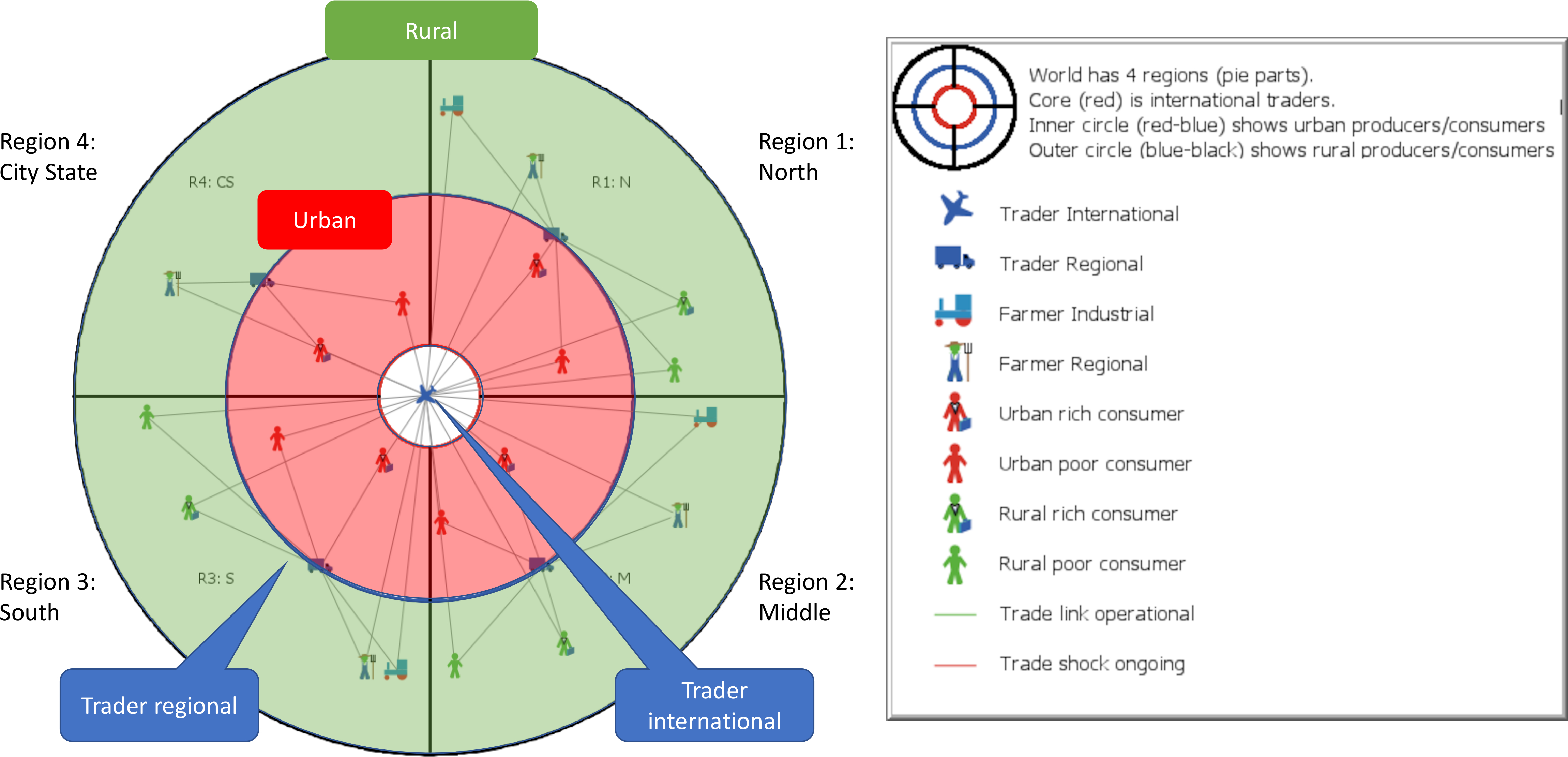
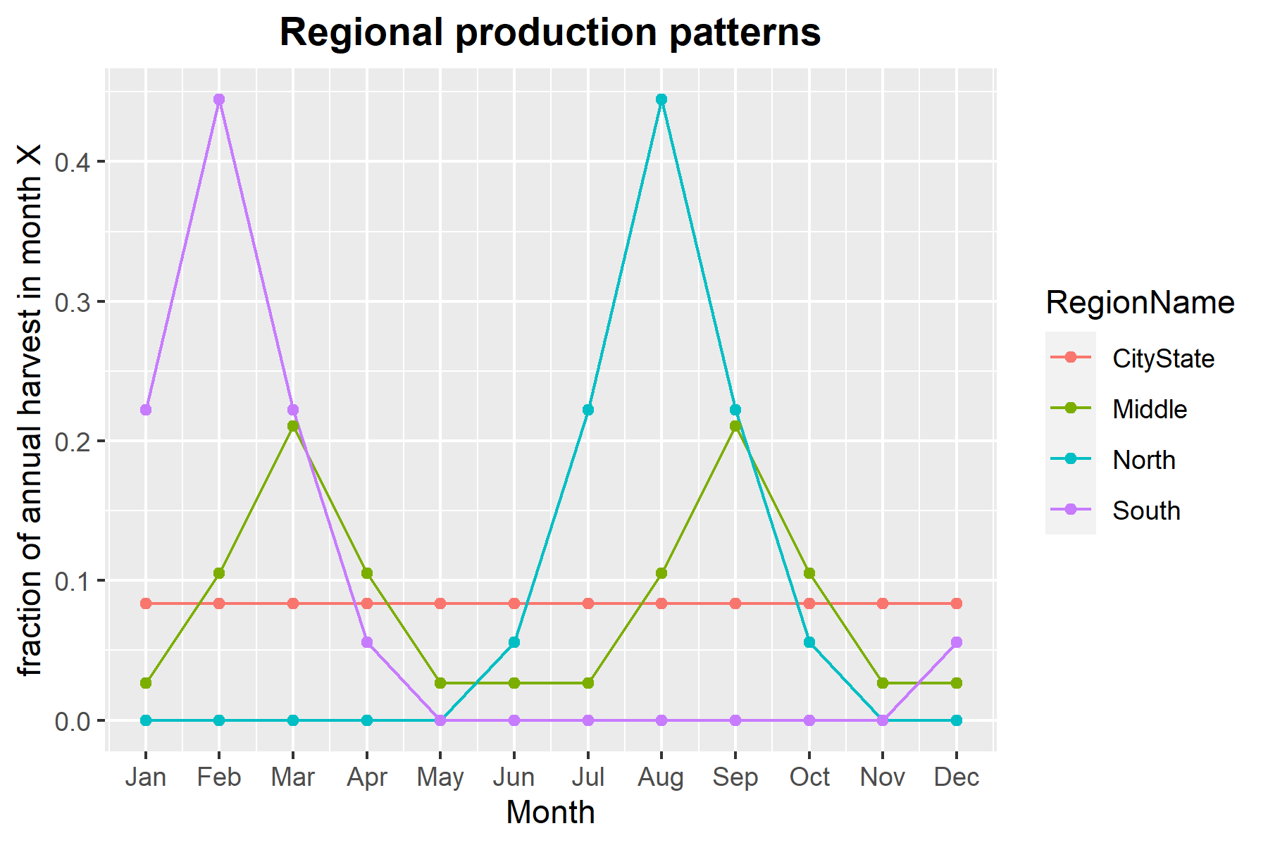
Figure 2 shows a schematic overview of the DARTS modelling framework. DARTS is not an acronym but instead is named after the pub game darts, because of the resemblance between a darts board and the visualisation of the simulated Worlds (see Figure 2). Each food system/‘World’ is subdivided into different regions with different concentric areas that indicate the difference between rural/urban/international trade areas. These areas are populated by different agent types. The number of agents and regions is defined in input files. For simplicity, Figure 2 shows only one agent per agent type per region. Each region has a rural area (outer green area) and an urban area (middle red area). Food producing agents are positioned only in the outer rural area. The World regions 1 to 4 represent a northern hemisphere region, an equatorial region, a southern hemisphere region and a city state, respectively, although some food Worlds do not include the city state. City states are distinct from other region because their rural population is near zero and their food production is substantially lower than other regions. The City states World was broadly inspired by countries such as Singapore, which do have some regional production, predominantly of perishable products like eggs and vegetables which are produced year round (Teng 2020). The differences across regions are mainly expressed through their different harvest months (Figure 3).
Comparison between food system archetypes/Worlds
Each World corresponds to the different food system archetypes shown in Figure 1. Our analysis is focussed on the impact of the structure of the global food system on its resilience. This structure we defined through:
- The distribution of the population over different agent-types, across the urban/rural divide and between regions,
- The trade-patterns between different regions and across the urban/rural divide.
To compare how food security is affected across the different food system archetypes in a consistent manner, we defined a set of parameters for population and food production, such that each World has the same properties at World scale when summed over all regions and agent types:
- World population: 12,000
- World food production: 42,022,840 MJ year\(^{-1}\)
- World food requirement: 37,440,000 MJ year\(^{-1}\)
- production / requirement: 1.12
The chosen World population was a compromise between precision and computational speed. Food production was set to a value larger than food requirement to account for food loss. Food production was set so that even in a World without shocks, a small fraction of World population would suffer from hunger periodically, when regional and/or international stocks run out. This serves to illustrate one important aspect of the DARTS model which is to show how intra-annual food security depends on intra-annual food stock dynamics. In the following sections, we present the parameters for the agents in the 4 Worlds (Figure 1) and the 4 regions within each World (Figure 2).
Agents
Each instance of DARTS is populated by two classes of agents: ConsumerProducers and Traders.
ConsumerProducers
ConsumerProducers aim to satisfy their food requirements by:
- Producing food
- Earning income by off-farm income or by selling food
- Maintaining a food stock and cash stock such that food requirements are met for the current and following month(s)
- Spend on non-food items
ConsumerProducers therefore hold two types of stock (cash and food). Consumers-producers are subdivided into 6 sub-categories, each with their own combination of food production capacity and off-farm income (food requirement is kept equal across ConsumerProducers): regional farmers, industrial farmers, rural poor, rural rich, urban poor and the urban rich.
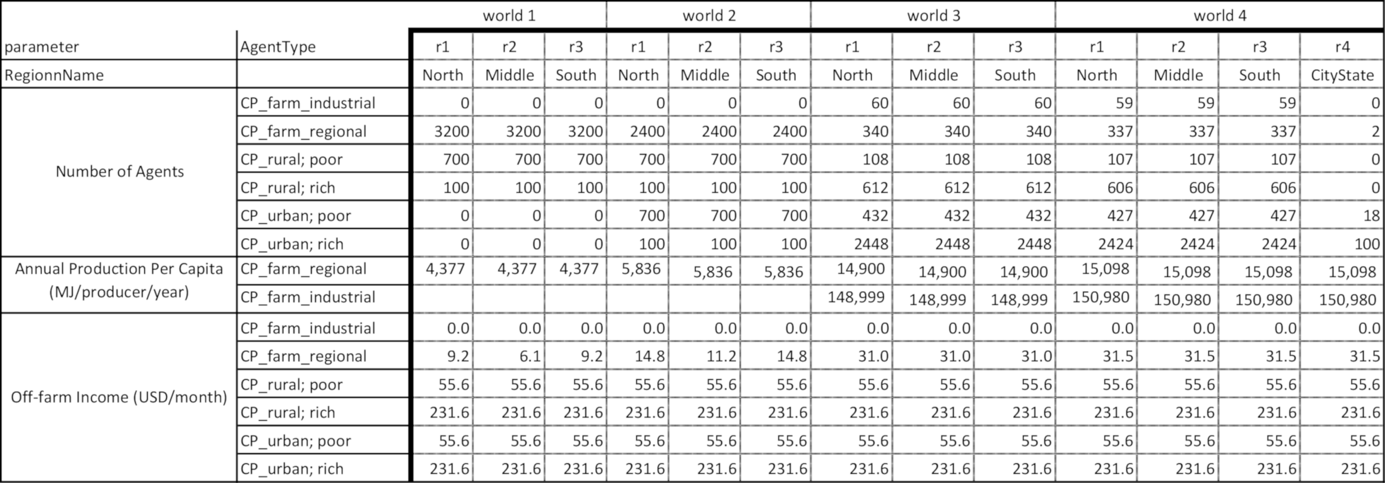
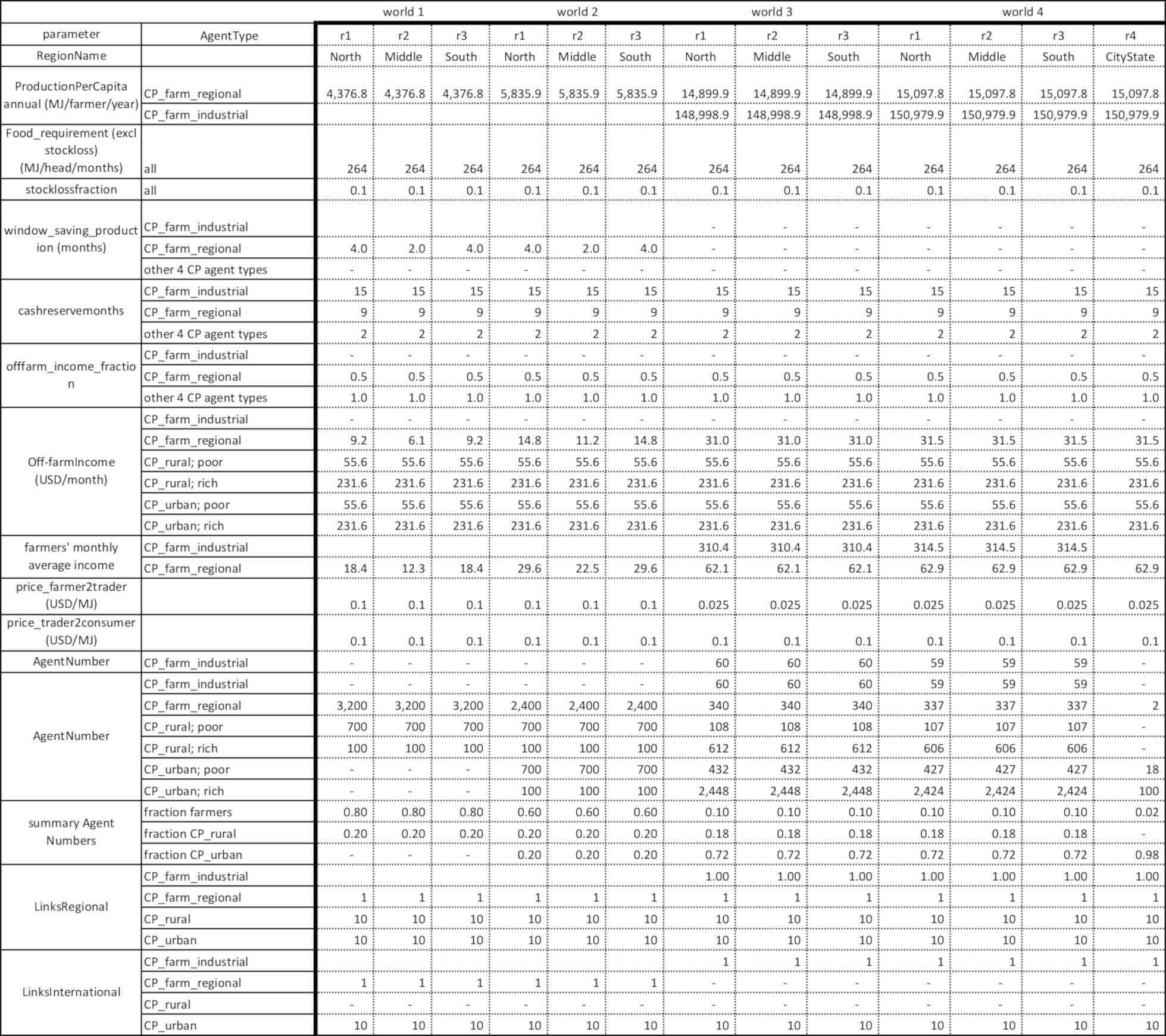
Table 1 lists a selection of the ConsumerProducers parameters in the 4 Worlds and 4 regions (see Table 6 in the ODD for full details). Table 7 list the rationale (often based on real-world data) for the derivation of the parameters. For instance, monthly production per farmer is calculated by multiplying the monthly harvest fraction with annual per capita production.
Traders and the trade network
Traders buy and sell food from and to ConsumerProducers. The price of food is fixed (Table 6). We define two Trader subtypes: international Traders (Figure 2: airplane symbol in the white core) and regional Traders on the border between the rural and urban ring (truck symbol in Figure 2). The subtype of the ConsumerProducer and Trader defines their trade links: regional farmers and rural consumers can only trade with regional Traders; whereas industrial farmers and urban consumers both preferentially trade with international Traders (but can also trade with regional Traders). These trade networks to a large extent mimic the situation in LMICs, where urban populations are more dependent on internationally traded food, but rural populations have lower access to internationally traded food and therefore depend more on local food production (Berazneva & Lee 2013).
Traders connect to all ConsumerProducers that they are allowed to link to following the rules described above: regional traders link to all consumers in their respective region, international traders link to industrial farmers and to urban consumers in all world regions. The number of Traders is defined in Table 2. Both Traders and ConsumerProducers hold stocks, which are prone to losses, thus Traders also have a stock loss fraction. Traders do not receive off-farm income and have no food requirement.
| parameter | Agent Type | world 1 | world 2 | world 3 | world 4 | unit |
|---|---|---|---|---|---|---|
| AgentNumber | T_international | 10 | 10 | |||
| T_regional | 10 | 10 | 10 | 10 | ||
| stocklossfraction | all | 0.05 | 0.05 | 0.05 | 0.05 | \(-\) |
Food security statistics
We quantify food security by averaging food satisfaction (defined as the amount of food consumed at the end of each month divided by the food requirements at the agent level) across regions and agent types. We average food satisfaction across the months following a shock to evaluate the immediate and longer-term effects of shocks. More specifically we compute a 3-months and a 12-months average food satisfaction as an indicator for short-term and medium-term food security.
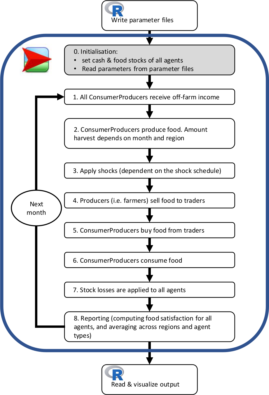
Simulation steps
Figure 4 shows the simulation steps. The main simulation is performed in Netlogo 6.2.0, initializing parameter files and post-hoc analyses are performed in R 4.2.1. We used the ‘snowfall’ package in R (Knaus et al. 2009) to parallelise computations. Each combination of World and shock scenario is run for 100 iterations with different random seeds. Although DARTS is largely deterministic, the ordering in which agents trade is random (for agents with equal properties). Running multiple iterations of the same world-scenario combination allows us to average across these stochastic effects. A closer analysis (not shown) revealed an inconsequential minor variation in model output over 100 iterations, hence here, we present only results as averages over the 100 iterations and not the range within the 100 outcomes per simulation.
ConsumerProducer agents (but not Traders) receive at each iteration a fixed off-farm income. This income is equal across agents within the same agent type but differs between agent types. The urban/rural rich receive more income than the urban/rural poor. Step 2 consists of food production. Each ConsumerProducer follows a production schedule, depending on their subcategory and region. Only regional and industrial farmers have non-zero production schedules. Step 3 applies shocks (if specified) to the agents. Shock types include production shocks (yield losses), trade shocks (e.g., export bans) and cash shocks (cash loss). Steps 4 and 5 constitute the trading steps. In step 4, each farmer (industrial first in random order, then regional in random order) visits all Traders to which she is connected (international Traders first in random order then regional Traders, in random order) and attempts to sell her surplus (production – food stock requirement). If the Trader has enough cash, the sale is concluded, otherwise the next Trader is visited. In step 5, each ConsumerProducer (ordered from high to low cash stock) visits the Traders to which she is connected (international Traders first, then regional Traders, both randomly ordered). See Section Sub-models in Appendix A: The ODD Protocol for a more detailed description of steps 4 and 5, including pseudo-code.
Four Worlds and their variations
The four food systems we study follow the archetypical food systems that we have introduced in Figure 1 and are hierarchically organised. We used a numbering scheme to denominate each World (see Table 3).
| u | Indicates |
|---|---|
| 1 | No urban population, No global trade links |
| 2 | 1 + urban population |
| 3 | 2 + global trade trade links |
| 4 | 3 + city state |
Scenarios: Baseline and export ban shock
Food security exhibits important dynamics during ‘business-as-usual’ scenarios and especially during shocks. The evaluation of food security during shocks is aided by direct comparison with a baseline scenario that is equivalent, except for the application of the shock itself. We therefore evaluated both a baseline and a shock scenario for all Worlds.
More specifically, the evaluation of baseline scenarios allows us to study the spatial and temporal dynamics of food security in food systems with varying degrees of trade connectivity. To what extent does trade mitigate temporal local shortages (hunger months) and is this mitigation effective for all groups within the food system? For the shock scenario, we have selected an export ban in the North, applied at June 1st (start of the harvesting season in the North) and continuing for 3 months. This allows us to investigate the resilience of groups across the food system against the first and second order effects of such an export ban. Shocks are applied during the 7th year of the simulation, to allow for initialisation effects to be minimised. Thus, the first month of the shock is the 90th month (7.5 \(\times\) 12) and we ended the simulation 12 months later (102th month) to allow for the evaluation of the 12-month average food satisfaction.
Scenario evaluation
For each scenario, we calculated food security (aggregated across agent types and areas/regions) over time and we calculated average food security over a 3-month and 12 month period starting in June of the 7th year of the simulation. The 3-month period of short-term food security measure coincides with the hunger months of the North, as well as with the moment of the application of the shock in shock scenarios.
Sensitivity analyses
We performed selective sensitivity analyses on the baseline scenario. The DARTS model presents a large parameter space to perform sensitivity analyses, so exhaustive sensitivity analyses are therefore computationally expensive. Moreover, many parameters are interdependent, which precludes manipulating one parameter while keeping others fixed. We have therefore performed sensitivity analyses for 5 parameters in a one-factor-at-a-time design (ten Broeke et al. 2016), while keeping all other parameters constant. These parameters are: N (total number of agents), the ratio of the total food production of a world and the total food requirement, the price traders pay producers for food (and by the same proportion the price consumers pay traders for food), the ratio of productivity or industrial versus regional farmers and the ratio of food spending for rich producers/consumers, which indirectly sets their off-farm income (see Table 7). We perform all sensitivity analyses on World 4 for the baseline scenario.
Results
We demonstrate the ability of DARTS to simulate food security for different food systems under a variety of different scenarios by running two scenarios and analysing the outcomes in-depth for each food system x World combination.
Baseline
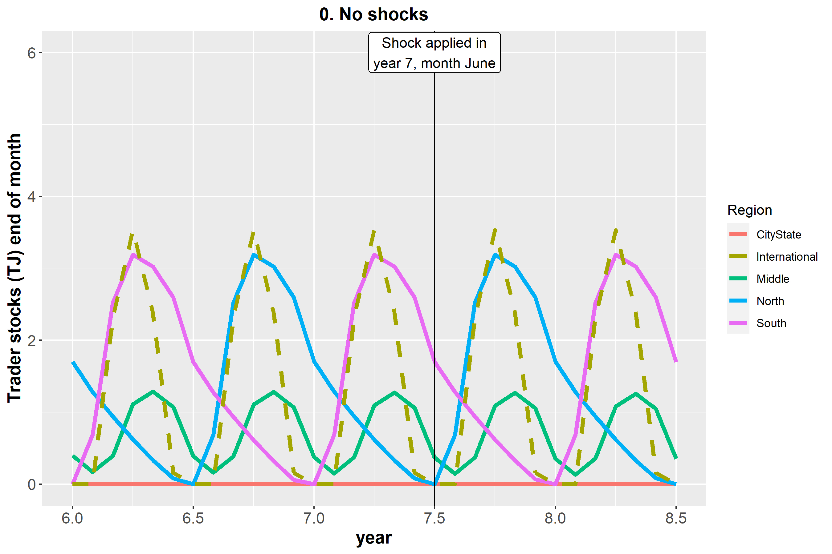
Stock dynamics
Figure 5 shows how regional and international stocks fluctuate within the year in World 4 for the Traders. ConsumerProducers are not shown since they hold no stock by the end of the month in World 4. In other Worlds (1 & 2), farmers do stock part of their harvest for their own consumption in which case, ConsumerProducers’ stocks do exhibit non-trivial dynamics. ConsumerProducers also hold stocks in case of hoarding (not considered here) or when farmers cannot export while at the same time regional Traders do not have enough cash to buy the food offered for sale by the farmers. Figure 5 shows stocks held at the end of the month, when both the trade from farmers to Traders and from Traders to consumers has been completed. This leads to a small lag visible between Figure 3 and Figure 5. The North already harvests in June (Figure 3), all of which is sold to the international market in June, which in turn is immediately bought by urban consumers around the World, leading to a zero international stock in year 6.5 and 7.5 in Figure 5.
Figure 5 shows two critical moments for food security in World 4. In June, the North is faced with both low regional stocks and low international stocks. The South experiences the same critical moment in December. The Middle region experiences two moments per year when stocks are low, in July and January, but regional stocks are never completely empty, indicating that there is always sufficient food available. Finally, the City State is vulnerable whenever international stocks are low, since it depends predominantly on international markets. The World presented here is simple with only 3 food producing regions (North, Middle, South) with harvest seasons as shown in Figure 3. A model containing more regions with more variation in harvest seasons would lead to a smoothing out of stock dynamics compared with the dynamics shown in Figure 4, i.e., with lower peaks in March/Sept and showing less depletion in June and December.
Food security fluctuates throughout the year along with these stock dynamics. This is one of the reasons for studying intra-annual variation in food security. The 3-months and 12-months average food satisfaction are shown in Figure 6 and Figure 7 and discussed in the following sections.
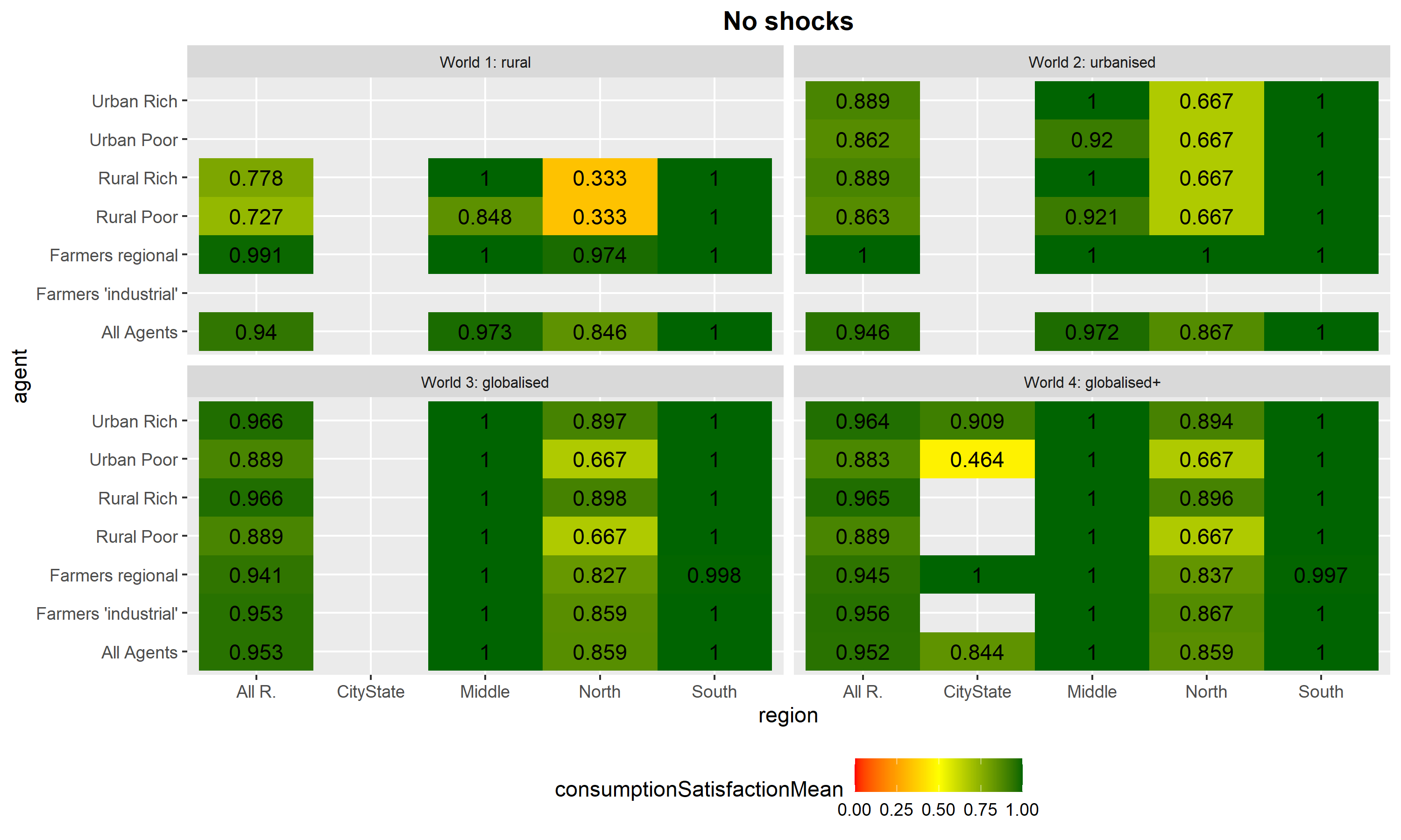
Baseline 3-months average food satisfaction
Figure 6 shows that for the 3-months average food satisfaction, only in the North region is food satisfaction below 1. This is caused by the alignment of the measurement period with the hunger months. The effect of this alignment differs across groups and Worlds and will therefore be addressed separately for each group \(\times\) World combination. In the first two Worlds, there is no trade between regions and ConsumerProducers only trade within their own region. The effect of the hunger months is therefore most pronounced in these Worlds, since rural and urban groups fully depend on trade with farmers in their own region. In the first months of the harvest period, farmers produce a limited amount of food, which they keep as stock for their own food security. This means that in World 1, for the first 2 months of the evaluation period no food is available for trade to rural consumers, which leads to low average food satisfaction (Figure 6, World 1, North: 0.333). In World 2, the regional farmers are more productive and support a larger proportion of non-food-producing agents. This means that the share of production the farmers stock for their own food security decreases, which leads to more food on the market earlier in the harvest months and a less severe reduction in food satisfaction for the non-food-producing agents (rural/urban poor/rich, 0.667 for all agent types). In Worlds 1 and 2, there is no difference between the rich and poor, because both are faced with a complete lack of food in the last of the hunger months, and therefore differences in cash holdings do not play a role.
World 3 shows the effect of integration between the regions by international trade. Compared with World 2, overall food security changes little (from 0.946 to 0.953) and also the food security of the North changes little (from 0.867 to 0.859). The first big difference between Worlds 2 and 3 is that differences appear between rich and poor. These differences hardly exist in Worlds 1 & 2, whereas in World 3, the rich are much better of than the poor. A second big difference is that in World 3, farmers are more food insecure. The latter occurs because we have deliberately chosen to decrease the food stocks that farmers will seek to hold. This is in line with modern trade where farmers generally sell all their produce and where farmers specialise in (cash) crops and rarely produce the full set of crops for a complete and healthy diet. Modern farmers like modern consumers, buy their food on the market rather than sourcing it from their own stocks. This means that during the harvest months, more food becomes immediately available on the market and that the farmers themselves suffer from shortages on these same markets. In Worlds 1 and 2, the North faces hunger in June because domestic stocks are depleted. In World 3 ideally hunger would be less if North could buy from the international market at a time when domestic stocks have run out. However, with the current parameter settings, coincidentally international stocks are also depleted in June (Figure 5). In this case, the international market provides no relief to all inhabitants in the North. The rich in the North do benefit from international trade (overall satisfaction increases from 0.667 to 0.897), but this improvement for the rich is offset by worsening food security of farmers in the North.
World 4 differs from World 3 only by the introduction of a City State. Urban consumers in the city state are almost completely dependent on the international market. Urban poor in the City state are particularly vulnerable since in this international market they compete unsuccessfully with the urban rich in their own region and with the rich in the other regions of the world. This is reflected in the low satisfaction of 0.464 for the City state urban poor.
Baseline 12-months average food satisfaction
Figure 7 shows the 12-months average food satisfaction for all Worlds in the baseline scenario. Despite World production being 12% higher than World food requirements, all Worlds experience moments of food shortage, which must be caused by stock losses and by food not being in the right place at the right time. Global mean annual food satisfaction is 0.917 in Worlds 1 and 2 and it is 0.973 in Worlds 3 and 4 indicating higher overall food security in these Worlds with international trade.
For Worlds 1 and 2 (no international trade), Figure 7 shows equal food satisfaction (0.882) between the North and South region. In these Worlds, the Middle regions shows highest overall food satisfaction (\(> 0.98\)). In the Middle region, two harvests are available per year instead of 1 in the North/South regions. During the first harvest months, farmers in North/South regions stock more food (since they need to survive more months without harvest) than farmers in the Middle region. Therefore, in the Middle region, food reaches the regional markets earlier, which reduces the impact of hunger months. Furthermore, with food being stocked for longer in the North and South (from one harvest to the next), total stock losses are also larger in the North and South than in the middle region with two harvests per year. Farmers in the North/South show higher food satisfaction than the other groups, because they stock food for almost as long as needed. In World 2, it is interesting to note that there is no difference between urban and rural. In these Worlds, there is no international market and therefore not difference in market access between rural and urban populations.
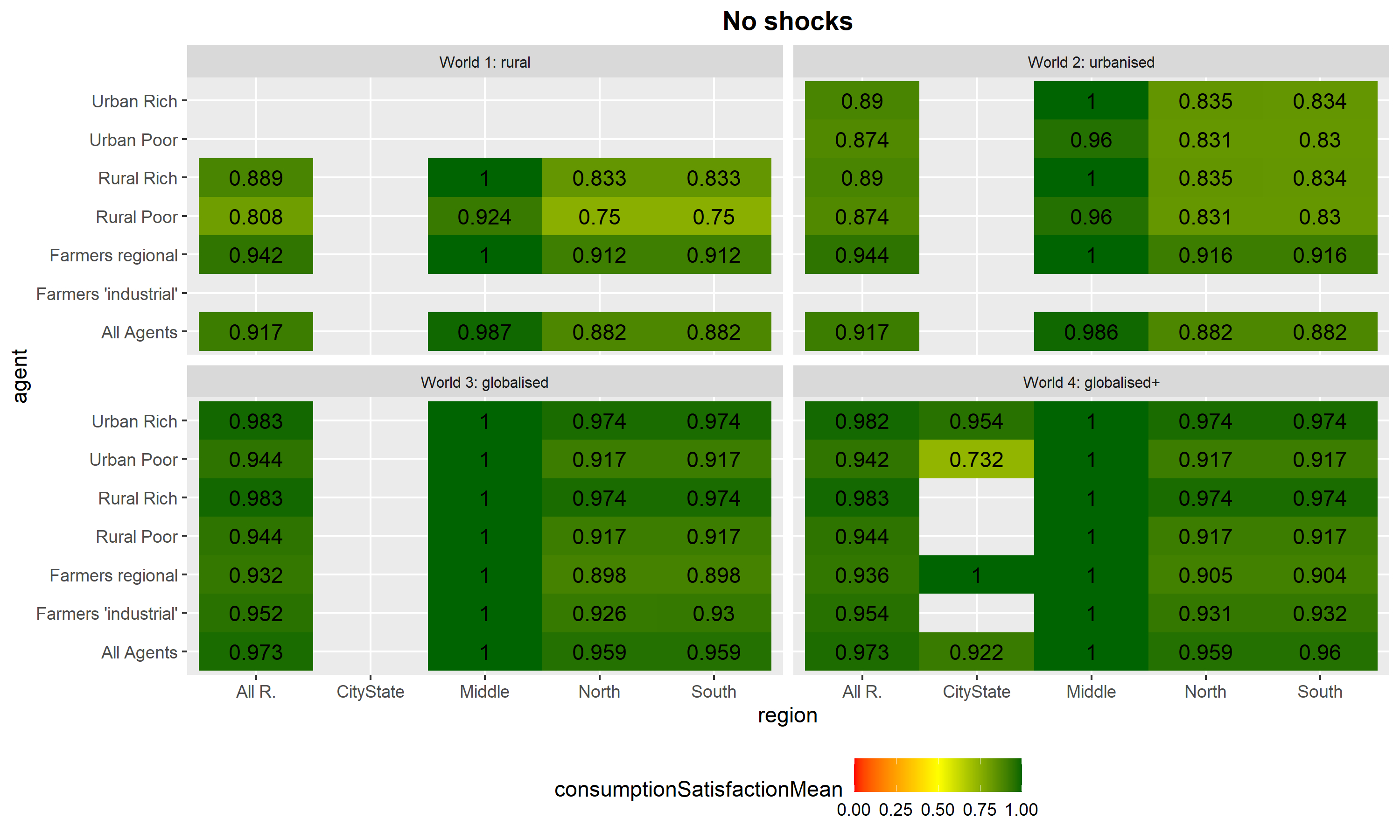
In Worlds 3 and 4, the introduction of the international market increases overall food security (from 0.917 in Worlds 1 and 2 to 0.973 in Worlds 3 and 4). This improvement is most pronounced in the North and South regions (satisfaction increases from 0.882 to 0.959). In the North/South regions, the farmers now show a slightly lower food satisfaction compared to the other consumer groups. In these Worlds, farmers do not stock food for their own consumption but sell everything immediately to the market. In Worlds 3 and 4, urban and rural consumers show the same food satisfaction (for instance, in World 3 urban/rural rich = 0.974, urban/rural poor = 0.917). Urban consumers preferentially shop internationally. This reduces pressure on regional markets. In months where the international markets are well stocked, this leads to maximum food satisfaction for urban and rural consumers. When the international markets are depleted, both urban and rural consumers trade on the same regional markets with the same income, therefore there are no differences between both populations.
World 4 shows only substantial differences with World 3 in the City State populations. In World 4, the urban rich of the City State show slightly lower food satisfaction (0.954) than the urban rich of the other regions (0.974), which is caused by their lack of recourse to a (significant) regional market in times when the international markets are depleted. In World 4, the urban poor are the most vulnerable population in this World (food satisfaction of 0.732), since they cannot fall back to their own regional market.
Shock scenario: Export ban for farmers in the North
We now analyse the effects of a shock scenario where farmers in region North cannot trade with the international market during their harvest months. In the following, we analyse differences in food satisfaction with respect to the baseline scenario.
Shock scenario: Difference in 3-months average food satisfaction to Baseline scenario
Figure 8 shows the difference in food satisfaction between the shock scenario and the baseline scenario. For Worlds 1 and 2 there is no difference, since in these Worlds there is no international markets and export bans have no effect. In World 3, there is no effect in the North as consumers in the North only suffer from low food satisfaction during the hunger months, in which export plays no role. The South and Middle regions do experience increased food insecurity (Middle/South = -0.212/-0.097), since the export ban in the North decreases the availability of food on the international market. The urban/rural poor in the Middle region (-0.546) show a higher decrease in food satisfaction than the South region (-0.333). This difference is caused by the fact that both regions rely more heavily on their regional markets at the time of the shock. However, the stocks of the regional Traders in the Middle region are smaller because food production in the Middle is more spread out (over two harvest seasons), which leads to lower maximum stocks. The regional farmers in the South region also show a substantial decrease in food satisfaction (-0.35). The shock occurs during a period that is outside the Southern harvesting period. In Worlds 3 and 4, the farmers do not stock food they produce, but sell all of it to the market, mimicking practices in the industrial World. Therefore, if international stocks are less available than is normally the case, the South (including their regional farmers) have to rely on regional markets for buying food, which is depleted during the shock.
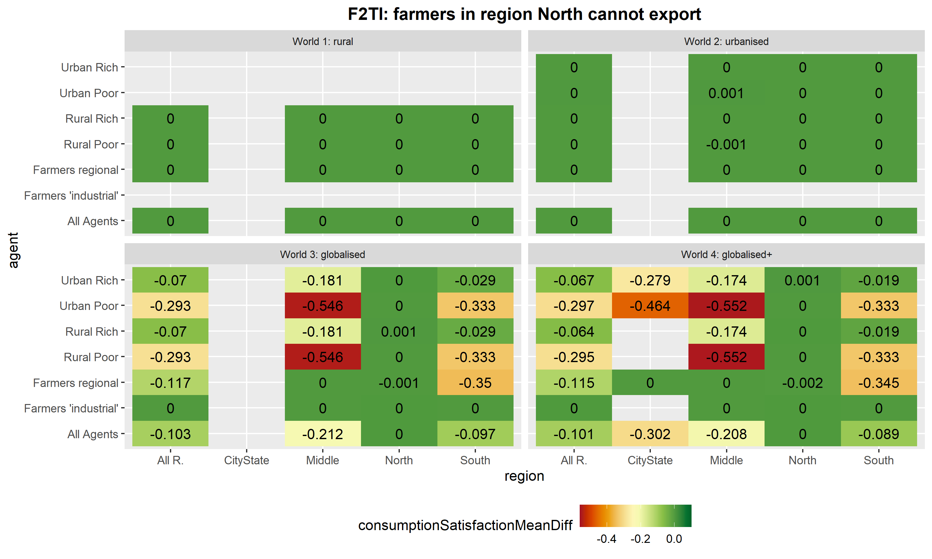
The addition of the City State in World 4 demonstrates the consequences of relying solely on international markets in this World. When supply to these markets is lower (due to the export ban in the North) and there is no alternative regional market, even the Urban rich show a substantial decrease in food satisfaction (-0.279), in contrast to the other regions, where the Urban poor/rich also have access to their respective regional markets. This effect is even stronger for the urban poor in the City State (-0.464), because of their unfavourable income position.
Shock scenario: Difference in 12-months average food satisfaction to Baseline scenario
Figure 9 shows the longer-term effects of the shock scenario when compared to the baseline. Again, Worlds 1 and 2 show no effect, since export does not play a role in these Worlds. In Words 3 and 4, the export shock leads to an increase in regional stocks in the North (slightly benefiting the Northern farmers) but, more importantly, to a decrease in the international stocks, which severely affects the other regions (for instance in World 3, Middle/South = -0.165/-0.166). It is interesting that this redistribution has such profound asymmetrical effects on food satisfaction. The effects of the export ban are largely comparable between the Middle and South regions, since they depend equally on international markets for their food security.
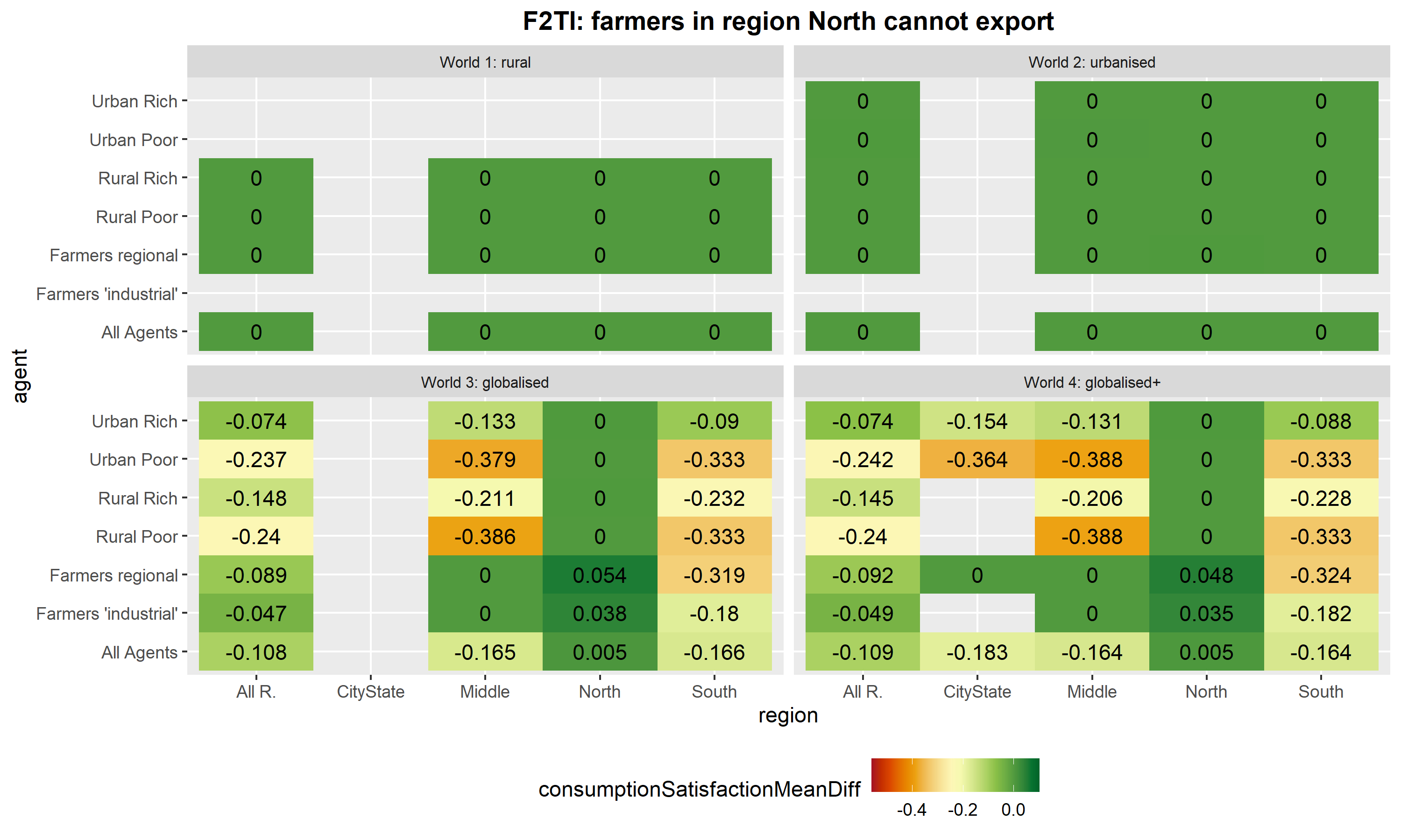
Figure 10 demonstrates further temporal effects of the export ban for World 3. In the North, the normal hunger months at the end of the 12 months following the shock disappear, since regional stocks have been unusually high because of the export ban. The Middle and the South regions experience the opposite effect, as since international stocks have not been sufficiently supplied, the Middle and South experience extensive (and recurring) periods of decreased food satisfaction. The Middle region benefits from harvests in the middle of this 12-month period, whereas for the South, the harvest period only occurs at the end of the evaluation period.

Sensitivity analyses results
Figure 12 in Appendix B: Sensitivity Analyses shows the results of the sensitivity analyses. Varying the total number of agents in the simulation (\(N\)) leads to negligible differences in food satisfaction, demonstrating that \(N=8000\) or \(12000\) is sufficiently high to avoid possible numerical artefacts that may occur with very low \(N\).
The ratio between the total food production in the world and the total food required in the world has a substantial effect on food satisfaction: reducing production increases hunger across the world, whereas with increased production hunger disappears. However note that this effect is non-linear, saturating. Overall satisfaction strongly increases from 0.771 to 0.953 (+0.184) along with a global production: requirement ratio increasing from 85% to 105%. When there is not enough food in the world, increasing production helps. Further raising the production: requirement ratio from 105% to 125% has little effect, because already almost all agents are at their maximum satisfaction of 1.0. And so, with a production: requirement ratio increasing from 105% to 125%, overall satisfaction increases only from 0.953 to 1.0 (+0.047). Comparing the 85% and 105% scenario we can see especially the food security of the poor improves, which is consistent with the model assumption of the poor being last in cue for food purchases. Recall the current sensitivity analysis is for the baseline scenario in which all trade links are effective. One could readily imagine that increasing production would not be effective in case of broken or dysfunctional trade links. Once again, this highlights how sensitivity analyses outcomes could be quite different depending on combinations of parameters (food systems architecture and food production). Something which also seen in the comparisons between worlds, where for the same global production: requirement ratio of 105%, overall satisfaction is higher in a world with globalised trade (Figure 7, Worlds 3 & 4) than in worlds without global trade (Figure 7, Worlds 1 & 2).
Varying food prices by \(\pm\) 50% (compared to the price used in the main results) has minimal effects on food satisfaction, demonstrating that in this price range, food satisfaction in relation to cash holdings of consumers is mainly affected by the order in which the consumers trade (rich consumers first). Note though that in the current configuration the poor spend 50% of their income on food (Appendix A: The ODD Protocol, Figure 11). Therefore, if prices increase by a factor of 2 (+100%), the poor would be spending all of their income on food and if prices increase by more than 100%, incomes of the poor would be chronically insufficient and we would expect satisfaction to become sensitive to even the smallest changes in the food price parameter. We can further deduce that, if food prices increase by more than 100% in region A, food purchases from region A would drop leading to more food available on the international market and thus the poor in other regions might benefit, thus dampening global effects of local price increases. More elaborate sensitivity analyses with wider parameter ranges and parameter changes in particular regions only were beyond the scope of the current simulation but illustrate the interconnectedness of food security around the world and the non-linear relations between parameters and food security that exist for many of the DARTS parameters.
The combination of lower industrial production and higher regional production leads to higher incomes for the regional farmers which in turn leads to higher satisfaction for the regional farmers. This combination leads to less food on the international market which, in turn, leads to decreased food security for the urban poor in the City state. The opposite combination (higher industrial production, lower regional production) leads to the opposite effects, i.e., improved food security for the poor in the City State, because of increased international trade, but decreased food security for the regional farmers (due to lower incomes), overall resulting in a slightly increased average world food satisfaction. Finally, changing the income of rich consumers does not change global food satisfaction, but does lead to a small shift in satisfaction between rich consumers (small reduction in satisfaction) and the industrial farmers (satisfaction increases slightly). Such a shift in food security between industrial farmers and rich consumers occurs because for a large part of the year, industrial farmers have higher savings, which positions industrial farmers ahead of rich consumers in the queue of agents visiting traders when purchasing food.
Discussion
This paper has introduced an agent-based model, DARTS, which provides an in silico laboratory for studying the effects of different trade architectures and other design factors on the resilience of food systems. Resilience in food systems is interpreted as the immediate and second order effects of shocks on the ability of populations to satisfy their food requirements. Here, we introduced the model by analysing the effects of two stylised scenarios: a baseline scenario without shocks and a scenario in which the North imposes an export ban. In the baseline scenario, the endogenous temporal dynamics of production, stocking, trade and consumption cause temporary drops in food satisfaction (i.e., hunger months). In contrast, the export ban scenario shows widespread decreases in food satisfaction, but only in Worlds where international trade is important. It is especially interesting to see that the export ban leads to second-order effects, in which food satisfaction returns to baseline levels after the immediate shock but then again drops.
Although generated by a simplified, abstract model, such second-order effects (or ripple effects) are seen in real-World food systems as well. The 2007-2008 global food price crisis started locally with droughts causing reduced harvests in some exporting countries, but then quickly became global when multiple exporting countries imposed export bans to secure the food supply of their own populations (Dawe 2012). Moreover, the trade-off between food systems depending on local production (Worlds 1 and 2) and food systems with international trade (Worlds 3 and 4) is already clearly demonstrated by the two scenarios. International trade provides some protection against the effects of the hunger months but can make populations vulnerable to export policies in other countries/regions. Although the fact that export bans only affect Worlds with international trade is trivial, it is instructive to analyse the different fates of poor and rich consumers in Worlds 3 and 4. Because of international trade, all consumers that are linked by international trade effectively act on the same markets and their absolute wealth differences determine whether they can purchase food. This suggests that international trade is only beneficial to food security, insofar as the population it concerns is sufficiently wealthy to compete on the international market place.
DARTS adds to existing food systems models by its emphasis on trade links within countries/regions: whereas many models focus on the household level, with few to no details on the trade arrangements between these households, or the country level, which leaves the distribution of food within countries unexamined, DARTS explicitly models trade between households within and across regions. However, it is extremely difficult to obtain data for this intermediate level of trade, as this would require access to the trade data of many private actors both in urban and in rural areas. DARTS can simulate intra-annual dynamics of regionally and internationally held food stocks (Figure 6). Quantitative data on stock dynamics are critical for understanding fluctuations of food security within the year, yet empirical data on government and privately held stocks are currently difficult to obtain. DARTS therefore contains only a relatively coarse description of the trading process, but which still allows an examination of the effects of local and global shocks.
DARTS keeps the behavioural affordances of the agents simple, i.e., agents can produce food, receive a fixed off-farm income and use the thus obtained financial means to satisfy their food requirements. Thus, DARTS focuses on the capacity of agents to absorb the shocks, both in terms of their food/cash stocks and their integration into local and global trade networks. DARTS therefore does not address adaptive and transformative capacities that are often discussed in the resilience literature (Folke et al. 2010). These capacities include the ability to adopt the agents’ earning capacity (e.g., new forms of production, different off-farm income opportunities) or the potential to migrate to different regions. However, including these possibilities would move the focus of the study away from the immediate impact of the shocks and substantially increase the behavioural complexity of the agents. Few agent-based models include such complexity and it would be difficult to argue for instance the empirical grounding of behavioural rules that decide migration decisions (but see Klabunde & Willekens (2016) for an overview of models for decision making in ABMs of migration). Moreover, including migration (most probably rural to urban) into the model would also require incorporating the effects of both a less populated rural area (does land ownership accumulate to the agents that remain?) and a more populated urban area (are there sufficient job opportunities for the arriving agents, does an increased labour force put pressure on their income?). These are all important and fascinating questions that will be addressed in future iterations of DARTS.
Another area of (deliberate) behavioural simplicity is trade: i.e., prices are set a priori and agents form a queue at their linked Traders in order of their cash holdings. Rich ConsumerProducers trade first and poor ConsumerProducers trade later and therefore more likely to encounter empty stocks. A mechanism for price discovery would be a more elegant solution and such mechanisms are indeed implemented in some agent-based studies (e.g., Farmer et al. 2005). Future work will explore which market microstructure is most suitable in the context of DARTS.
Agent-based models exist in many different forms. One dimension to categorise ABMs is with respect to their intended realism: empirical ABMs (Smajgl & Barreteau 2017) ideally include both data to inform behaviour at the agent-level (in essence what decision models are used and how they are parameterised) and data on the macro-level behaviour of the system under investigation. The macro-level data can consist of stylised facts (e.g., wealth distribution generally follow power laws) but also macro-level data (economic output, food security) that are both time- and place-specific. A different class of models sacrifices realism and focuses on simple and abstract descriptions of systems and their ability to reproduce stylised facts (for instance the Sugarscape model by Epstein & Axtell 1996). Such models are believed to be more easily generalizable, especially if the stylised facts are replicated over many different parameter initialisations, but the stylised facts that can be reproduced by these models are often very general. DARTS leans more towards the abstract and simple class of ABMs, mainly because detailed trade data are missing from real-world food systems. Moreover, DARTS was specifically designed to study a range of food systems archetypes. In each DARTS World, parameter initialisation was informed by real-world data as much as possible, but in many cases, guesstimates were necessary where real-world data were not readily available.
We acknowledge that, just as the original sugar-scape model is not a realistic land-use model, DARTS does not provide a representation of the real-world food trade system, which is in reality far more complex than represented here in DARTS. Rather, the model and its simulations can be considered a thought experiment that, with all the caveats and abstractions noted, can help to understand how global food security can be influenced by trade-links, urbanisation, harvest patterns, food reserves held in different parts of the world by different agents, agents’ wealth and shocks in this food system.
In conclusion, this paper has introduced and described the DARTS modelling framework in detail and has demonstrated its behaviour by analysing two scenarios. Follow-up work will focus on a broader set of shock scenarios (including shocks to productions and trade links) and will generalise the effects of these scenarios to evaluate the resilience of the food system archetypes against the full set of shock scenarios.
Acknowledgements
We like to thank the editor and the two anonymous reviewers for their thoughtful comments. The authors would like to acknowledge funding for project KB35-103-002 from the Wageningen University & Research "Food and Water Security programme" that is supported by the Dutch Ministry of Agriculture, Nature and Food Security.Code Availability
Model code is available at: https://www.comses.net/codebases/62b474c3-9247-4265-88d7-ea7472d5e1ab/releases/1.0.0.Appendix A: The ODD Protocol
Purpose and patterns
The purpose of this model is to illustrate how food system architecture influences the resilience of groups within this food system. Food security is generally expected to increase with increasing integration of all actors within a food system. However, our global food system sees groups with persistent low food security and resilience. This model investigates the interplay between connectivity and food security and resilience in the presence of unequal distribution of wealth and (food) productive capacity. Resilience is evaluated with respect to a variety of local and global shocks.
Entities, state variables and scales
Spatial units
Agents in DARTS occupy one of four different regions (North, Middle, South and City State) (see Figure 2) and one out of two different zones within these regions (rural and urban). This combination of spatial information determines the presence of certain agent types and a number of the agents’ state variables (e.g., off-farm income, harvesting months, etc.). The spatial location of agents within their region and zone does not have implications for their functioning and is only varied for visualization purposes.
Agents
There are two distinct types of agents within DARTS: ConsumerProducers and Traders. ConsumerProducers have varying capacity to produce food but all are required to consume food. Traders buy and sell food from/to ConsumerProducers with which they are connected and are not required to consume food.
Collectives
ConsumerProducers can be further subdivided into farmers (producing food) which in turn can be subdivided with respect to their productive capacity and trade connections into regional and industrial farmers. ConsumerProducers who do not produce food are Consumers, which can again be subdivided into rich/poor urban/rural Consumers.
Traders can be subdivided into regional traders, who are situated within a specific region and international traders, who trade between regions.
The network is structured such that regional farmers and rural consumers can only trade through regional traders, but industrial farmers and urban consumers can trade with both regional and international traders.
Environment
The observer records data for each ConsumerProducer/Trader and sets global variables such as the buy/sell price for food (fixed for all agents and all time steps of the simulation).
Attributes
Table 4 and Table 5 show the agent attributes for the ConsumerProducer and Trader agent types. Food represents a summary food type that satisfies all nutritional requirements of the agents with one stock. The processing of this food is left implicit as a trader activity.
| Name | Description | Static/Dynamic | Type | Unit | Range |
|---|---|---|---|---|---|
| Food | food available for consumption | Dynamic | floating-point number | MJ | [0-Inf] |
| Cash | cash available for spending | Dynamic | floating-point number | USD | [0-Inf] |
| food requirement | food required for consumption per month | Static | floating-point number | MJ | [0-Inf] |
| production | For each month, how much food does the ConsumerProducer produce | Static | floating-point number | MJ | [0-Inf] |
| off-farm income | How much does the ConsumerProducer earn in off-farm income | Static | floating-point number | USD | [0-Inf] |
| window-saving production | # months of food requirement that the agent aims to stock | Static | floating-point number | MJ | [0-Inf] |
| stock loss fraction | fraction of stock that is lost each month | Static | floating-point number | - | [0-1] |
| cash reserve months | cash amount above which non-food spending takes place (expressed in number of months of food requirement) | Static | floating-point number | Month | [0-Inf] |
| Name | Description | Static/Dynamic | Type | Unit | Range |
|---|---|---|---|---|---|
| food | food available to sell | Dynamic | floating-point number | MJ | [0-Inf] |
| cash | cash available to buy food with | Dynamic | floating-point number | USD | [0-Inf] |
| stock loss fraction | fraction of stock that is lost each month | Static | floating-point number | - | [0-1] |
Scales
Each time step within DARTS represents a month. This allows for the representation of different harvest months across regions and especially for the occurrence of hunger months in the months leading up to the harvest. Each simulation runs in total for 102 months, of which the first 89 months serve as an initialization period, during which no shocks occur. The shock is then applied consistently on the 90th, which aligns with the start of the harvest season in the north. All shocks are specific to regions and need therefore to be aligned in some cases (production shocks) to the harvesting period of that region. We maintain the starting time of the shock across shocks for consistency reasons.
Space is principally used to order the agents according to their trading relationships, productive capacity and earning capacity as outlined in Collectives. Regions govern trading month (the North and South have a single harvesting season starting in June/November respectively, the Middle region resembles an equatorial region with two harvest seasons starting in January and July and the City/State has constant production. The rural/urban zones within each region governs the presence of farmers (rural) and the trade relationships (rural ConsumerProducers only trade with regional Traders, urban ConsumerProducers trade with both regional and international traders). International traders occupy an (unnamed) international trade zone that is not unique related to any of the regions.
Process overview and scheduling
At each time step, the agents execute the following processes:
- All ConsumerProducers receive off-farm income
- ConsumerProducers produce food according to their productive capacity for this month (cf. harvest months for the ConsumerProducers’ region, only farmers produce food)
- Apply shocks (dependent on the shock schedule)
- Producers (i.e. farmers) sell food to traders
- ConsumerProducers buy food from traders
- ConsumerProducers consume food
- Stock losses are applied to all agents
- Reporting (computing food satisfaction for all agents, and averaging across regions and agent types)
This process schedule thus divides the month in 4 phases: a production/off-farm income phase, a trade phase (both selling and buying food), a food stock reduction phase (both by consumption and by stock losses) , after which food satisfaction for all agents and their aggregates (type/region) is reported. All processes are kept as simple as possible, with little or no dynamics with respect to productive capacity (planning, putting more emphasis on off-farm income/food production) and trade (prices are fixed, no price discovery by agent interactions). The planning of activities of farmers (who engage in a mixture of food production and off-farm employment) can be considered constant during the shock itself and its immediate aftermath, which justifies keeping this mixture constant for the simulation. Trade could have been made more dynamic. However, price discovery mechanisms are likely very different between local markets (regional traders) and international markets (international traders, probably operating on the basis of commodity markets). Instead of price fluctuations, the agents are ordered with respect to their cash holdings when visiting traders to buy food, such that rich agents arrive first and poor traders arrive last, at which time the traders’ food stocks can be empty. Where in reality, food shortages lead to price increases, which makes food unaffordable for the poor, in our model food stocks are simply empty when the poor trade with traders.
Design concepts
Basic principles
Two important components of food security are availability and accessibility. Accessibility is determined by earning capacity and wealth and the configuration of the trade networks across regions and groups within those regions. Many models, both statistical and generative (cf. CGE models) describe and predict trade at the country level, since at this level the most detailed data exist on trade flows. DARTS disentangles trade within regions into an urban and a rural component and distinguishes between locally traded and internationally traded food. Moreover, most models describe trade at equilibrium; by employing an ABM, DARTS can evaluate food security during and after a shock. By simplifying the food system into a limited set of agent collectives and their connections, an intuitive methodology for shocking the system suggests itself: shocks can be applied on agent attributes or on the connections between agents. Thus, DARTS can be seen as an in silico laboratory to simulate the dynamic response of food systems with different levels of integration and distribution.
Emergence
Food security for each agent collective is an emergent property of the place the agent collective occupies in the trade network, its own productive and earning capacity and the particular shock that is applied. Immediate and longer lasting effects on food security are expected.
Adaptation
There is minimal adaptive behaviour of the agents which is purely focused on maintaining food and cash stocks at heights set at the beginning of the simulation. These stocks are useful at a later stage, when food is scarce.
Objectives
The primary objective of the ConsumerProducer agents is to satisfy their food requirements.
Learning
There is no learning in DARTS.
Prediction
Prediction is only implicitly present in the setting by the modeler of the size of the food stocks that should be maintained, which are calibrated to allow for hunger months right before the beginning of the local harvest months.
Sensing
The agents know the agents that they are connected with, but not the attributes they have. They know the region and zone they are in which determines their attributes (including the harvest months).
Interaction
Agents interact by trading food with cash as the intermediary.
Stochasticity
There is no stochasticity in the assignment of the agent attributes. However, the order in which the agents proceed through each step is random. When buying food from traders, the position within the queue of these traders is determined by agents’ cash holding, but is random for agents with equal cash holdings.
Collectives
See the section Collectives.
Observation
The observer records the food satisfaction (= food consumed/food requirement) for each agent separately and computes average food satisfaction across agent collectives and regions.
Initialization and input data
DARTS represents different archetypical food systems (or worlds) by varying the presence of different ConsumerProducer/Trader subtypes (starting only regional farmers and rural Consumers and hence no connections between regions and no City State) in the simplest world to a fully connected food system including all agent types and a City State region with low productive capacity on its own. The number of agents is kept constant across the worlds at 12000 agents in total.
Initialization includes setting distributing the agents across their regions and functions, and a number of their attributes depending on the World they inhabit. Table 6 provides an overview of the attribute values for ConsumerProducers and Traders. Table 7 and Table 8 describe the derivation of these parameters for the ConsumerProducers and the Traders respectively.
| Consumer-Producer parameter | Source |
|---|---|
| ProductionPerCapita annual | ProductionPerCapita annual was set such for any given number of farmers, global food production would be the same in all 4 worlds. A ‘modern’ world with less farmers will have a higher per capita production. Per capita production of the industrial farmers was set to a higher value than for the regional farmers. |
| Food_requirement (excl stockloss) | A daily food requirement of 2100 kcal/day (Willett et al. 2019) was converted to: 2100 kcal/day \(\rightarrow\) 30 \(\times\) 2100 \(\times\) 4.1868 \(\times\) 1e-3 = 264 MJ head\(^{-1}\) month\(^{-1}\). |
| Stocklossfraction | fraction of stock loss per month. Based on FAO (2011). Note stock loss is calculated AFTER consumption. Thus if during a the month an agent has managed to buy only 50% of his/her food requirement, 132 MJ, then all 132 MJ will be consumed and stock loss will be zero. If the consumer had enough cash and traders had enough food for sale then the consumer would have bought food_req / (1-stocklossfraction) = 277.9 MJ, consumed 264 MJ and lost 13.9 MJ (note 13.9/277.9 = 0.05 = stocklossfraction). A farmer stocking food for 4 months could have 264 $$4 MJ in stock, consume 264 MJ and then lose 0.05 \(\times\) 264 \(\times\) 3 = 39.6MJ. Next month this farmer would have (264 \(\times\) 4 - 264 - 39.6) = 752.4 MJ in stock, consume 264 MJ and then lose 0.05 \(\times\) (752.4 - 264) = 24.42 MJ, etc. Aggregate losses accumulated over multiple months will be larger than 5% |
| window_saving_production | Author’s choice. We presumed in the more rural non-globalized worlds farmers would stock a greater fraction of their harvest and sell the remainder. We presumed farmers in the ‘modern’ worlds are completely market oriented, selling their full harvest to traders. |
| cashreservemonths | A cash reserve of 2 months means an agent keeps enough cash reserves for purchasing 2 months’ worth of food, which depends on his/her food requirement and on the price at which food is purchased. The cash reserve parameter must be seen in the context of how we model agents’ cash over time. Each timestep agents receive income, spend cash on food and then, in a situation without cash reserves, spend the full remainder on non-food. This simpler approach results in very low cash for farmers with a variable income (related to harvest pattern within the year). And it results in strong sensitivity of non-farmers to income shocks. As a result, modelled food security was low for farmers, rural poor and urban poor. With a greater cash reserve these agents are less sensitive to variable income (farmers) or cash shocks (non-farmers). Especially for the industrial farmers with no off-farm income and with only one major harvest period per year, a high cashreservemonths is needed to ensure food security. cashreservemonths parameters for the various agents were chosen by the authors such that in the baseline world without shocks, food security risk due to lack of cash would be small. |
| offfarm_income_fraction | offfarm_income_fraction is an intermediate parameter. We used it to calculate the off-farm income (see below) which is actually used in the DARTS model as a parameter. We assume regional farmers gain 50% of their annual total income from food sales (only during the harvesting season) plus as a steady off-farm income. This 50% is in line with surveys from developing countries (e.g., Frelat et al. 2016). And it is in line with the situation in richer countries where farmers receive subsidies and/or run businesses aside from their farms. We assume industrial farmers, who sell greater volumes, completely rely on food sales for their income, i.e. they have no off-farm income Non-farmers have no farm income, so their off-farm income fraction is 1 |
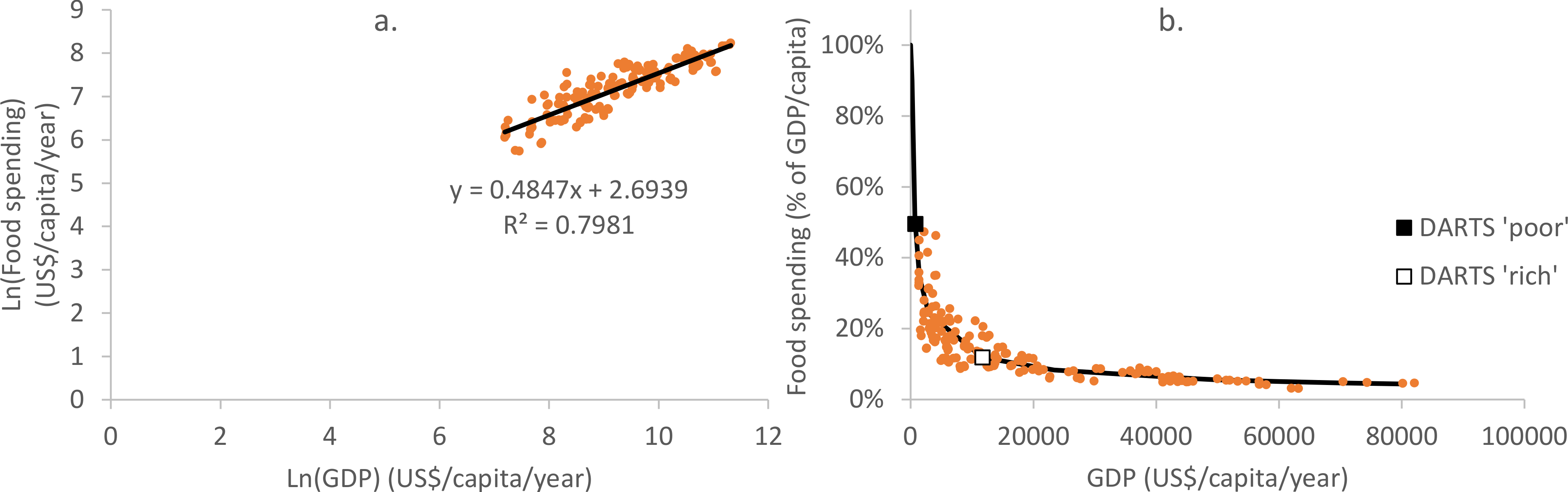
| Off-farm Income | Off-farm income of the non-farmers. Monthly off-farm income of the rich and the poor in our worlds was set such the fraction of income spent on food corresponds roughly with that of the rich and the poor in our world today (Figure 11). Then calculating backwards from food requirement and the price at which consumers purchase their food, we set non-farmers income (Table 6, Table 1) such that the fraction of their income spent on food matches that in the right panel of Figure 11. Off-farm income of the industrial farmers. This was simply set to zero, see above. Off-farm income of the regional farmers. For the regional farmers we assumed x% of their income was from food sales and x% from off-farm income. We first calculated their annual income from food sales which depends on production, consumption, stocking, losses and parameter price_farmer2trader. Once annual income from food sales was known the annual off-farm income could be calculated such that off-farm income would equal x% of total income. Monthly off-farm income was calculated by dividing annual by 12. |
| farmers’ monthly average income | farmers’ monthly average income in Table 1. We calculated it for comparison with the non-farmers monthly income. |
| price_farmer2trader | Cereals have ca 17 kJ/g = 17.0 MJ/kg (http://www.fao.org/3/y5022e/y5022e04.htm). Farmgate prices fluctuate wildly over time. A visual estimate of long-term average wheat farmgate prices (https://fred.stlouisfed.org/series/PWHEAMTUSDM) is 170 USD/ton = 0.17 USD kg\(^{-1}\) = 0.17/17 = 0.01 USD MJ\(^{-1}\). Wheat is amongst the cheapest agricultural food crops. Arbitrarily we assumed a 5x higher price to account for farmers also cultivating higher value crops, thus 0.05 USD MJ\(^{-1}\). Also, prices for animal products are higher than for wheat. With per capita production of the farmers being higher in the modern worlds we assumed lower farmgate prices in the ‘modern’ worlds 3 and 4, 0.025 USD MJ\(^{-1}\). |
| price_trader2consumer | Traders earn income from the services they offer which includes collecting food harvest from farmer, transport, stocking, processing and selling to farmers. We assumed in the ‘rural non-globalized’ worlds price_trader2consumer (0.1) would be 2\(\times\) higher than price_farmer2trader (0.05). In the ‘modern’ worlds price_farmer2trader is 2\(\times\) lower than in the ‘rural non-globalized’ world (0.025). At the same price_trader2consumer (0.1), food price quadruples (4\(\times\), from 0.05 to 0.1). Which is consistent with longer value chains (e.g., European people buying Australian wine) and consistent with modern food systems selling more processed food. |
| AgentNumber | Total agent number. The total agent number was set to the same value to allow for comparison between worlds, while admittedly human population is growing exponentially and thus a more realistic set up would be one with a growing world population. The choice of total agent number of 12,000 was a compromise between precision (which increases with agent number) and computational speed (decreasing with agent number). Evolution of food systems. To allow for a comparison between worlds, the same global population was used in all worlds. Within the worlds, distribution of the population among agent types was evolving: \(\cdot\) World 1 has only a rural population of which a relatively large fraction is farmer. \(\cdot\) World 2 has a 20% urban population, but all trade is still regional, i.e. there are no industrial (international market oriented) farmers and no international traders. \(\cdot\) World 3 has a 72% urban population and it has international traders. Note there exists no standard definition of "urban". In the DARTS context "urban" simply means being connected to the international market. Thus a small village in the Netherlands in which one can easily purchase food from any region in the world would classify as urban, even if the village population is small and even if the village is surrounded by vast areas of nature or agricultural production. According to the UN and summarised in https://ourworldindata.org/urbanization, the fraction of people living in urban areas will increase from 4.2/7.6 = 55% today to 6.7/9.8 = 68% in 2050. Our globalised world with 72% urbanisation comes close to this number. \(\cdot\) World 4 is very similar to World 3 (72% urban, international trade). In world 4, 3 \(\times\) 3960 = 11880 people live in regions 1 to 3 and population of the city state (r4) is 120 (1% out of 12000). Our world. Currently, depending on definition, the world has 6-10 City States (Bahrain, Hong Kong, Macau, Malta, Singapore, Monaco, United Arab Emirates, Andorra, Qatar, San Marino), 0.2% to 0.04% of world population. Our number of 1% is higher than this number but not very far off. |
| LinksRegional | For the non-farmers, each consumer was assumed to be linked to all available regional traders. Each farmer was assumed to be linked to only one regional trader. |
| LinksInternational | For the non-farmers, each urban consumer was assumed to be linked to all available international traders. Rural non-farmers were assumed to have no links to international traders. Each industrial farmer was assumed to be linked to only one regional trader. Regional farmers have no links to international traders. |
| Trader parameter | Source |
|---|---|
| AgentNumber | Producers and Consumer numbers exceeds the number of traders. Based on the hourglass network in van Voorn et al. (2020). |
| Stocklossfraction | Like farmers and like consumers, also traders suffer from stock losses. In an absolute sense these can be quite large as traders generally hold far greater stocks (in warehouses) than consumer-producers. The stockloss fraction was based on FAO (2011). |
| Consumption, non-food spending | The consumer-producer agent in the DARTS can be considered representing real human beings. The trader agent in the DARTS is more like an institution or service provider for which it was deemed less important to model their food consumption and non-food spending. In a way, one could think of part of the consumers being employed by these trader “institutions”. For this reason, we did not explicitly separately model consumption and non-food spending of this category of agents. |
Submodels
Steps 4 and 5 in section Process overview and scheduling require further elaboration.
ConsumerProducers buy food from traders
Industrial farmers trade first, then regional farmers. The order in which industrial and regional farmers trade within their category is random.
Each farmer performs the following steps:
- compute whether they have surplus food for trade by comparing their food stock with the amount of food they are intending to stock (window-saving production).
- If this surplus is larger than zero, they:
- visit the international traders that they are connected to in random order
- sell as much as they can to the trader they are visiting (determined by the price_farmer2trader and the cash holding of the trader) as possible
- visit the regional traders they are connected to in random order
- sell as much to each regional trader they are visiting (determined by the price_farmer2trader and the cash holding of the trader) as possible
The difference between the industrial and regional farmers is in the traders they are connected to: industrial farmers are connected to international traders and regional traders whereas regional farmers are connected to regional traders only. By visiting the international traders first, it is established that industrial farmers preferentially sell to international traders and that significant trade between industrial farmers and regional traders only occur during an export ban or when international traders have no cash. The preference for industrial farmers to service international markets mimics patterns of trade in modern food systems.
ConsumerProducers consume food
Each ConsumerProducer is sorted with respect to their cash holding. Rich ConsumerProducers trade first, then poor ConsumerProducers. ConsumerProducers with the same cash holding are sorted in random order.
Each ConsumerProducer then performs the following steps:
- Determine the amount of food that needs to be bought (determined by the food requirement, the stock loss fraction and the stocked food).
- Determine the cash holding.
- If the cash holding allows for buying food (even is this is lower than the amount of food that needs to be bought then:
- Visit connected international traders (random order within the international traders)
- Buy from international trader (determined by the price_trader2consumer, the cash holding of the ConsumerProducer and the food stock of the visited trader) the amount of food that needs to be bought (step 1) and stop shopping when (i) all that needs to be bought has already been bought or (ii) ConsumerProducer has run out of cash.
- Visit connected regional traders (random order within the regional traders)
- Buy from each regional trader (determined by the price_trader2consumer, the cash holding of the ConsumerProducer and the food stock of the visited trader) the amount of food that needs to be bought (step 1) and stop shopping when (i) all that needs to be bought has been bought or (ii) ConsumerProducer has run out of cash.
Appendix B: Sensitivity Analyses
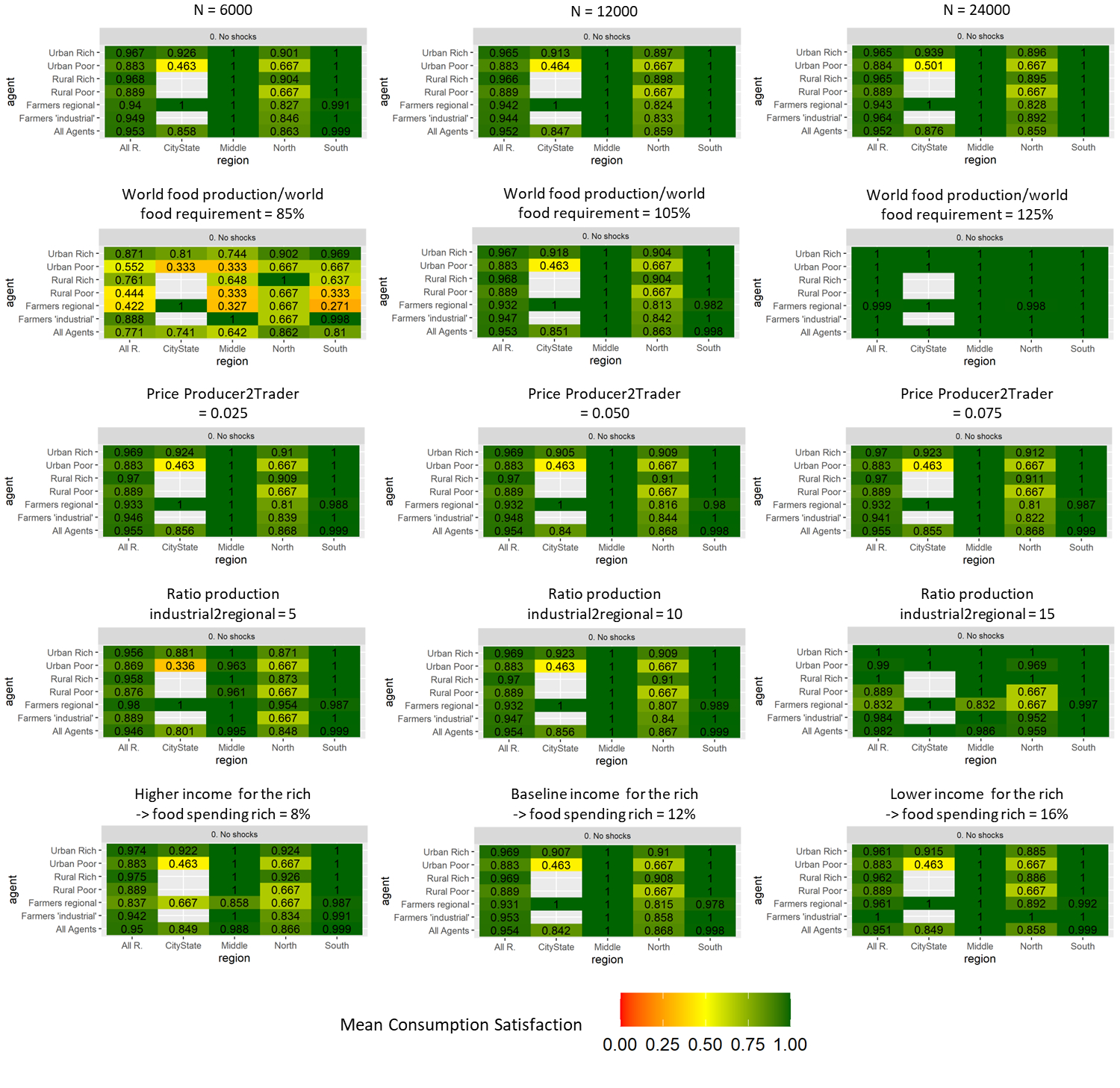
References
ANDERSON, K. (2016). Agricultural Trade, Policy Reforms, and Global Food Security. Springer: Berlin Heidelberg.
BERAZNEVA, J., & Lee, D. R. (2013). Explaining the african food riots of 2007-2008: An empirical analysis. Food Policy, 39, 28–39. [doi:10.1016/j.foodpol.2012.12.007]
COLLIER, P. (2007). The Bottom Billion: Why the Poorest Countries Are Failing and What Can Be Done About It. Oxford University Press: Oxford.
CONCEIÇÃO, P., & Mendoza, R. U. (2009). Anatomy of the global food crisis. Third World Quarterly, 30(6), 1159–1182.
D’AMOUR, C. B., Wenz, L., Kalkuhl, M., Steckel, J. C., & Creutzig, F. (2016). Teleconnected food supply shocks. Environmental Research Letters, 11(3), 035007.
DAWE, D. (2012). The Rice Crisis: Markets Policies and Food Security. Routledge: London.
DOBBIE, S., Schreckenberg, K., Dyke, J., Schaafsma, M., & Balbi, S. (2018). Agent-based modelling to assess community food security and sustainable livelihoods. Journal of Artificial Societies and Social Simulation, 21(1), 9. [doi:10.18564/jasss.3639]
DOLFING, A. G., Leuven, J. R., & Dermody, B. J. (2019). The effects of network topology, climate variability and shocks on the evolution and resilience of a food trade network. PLoS One, 14(3), e0213378. [doi:10.1371/journal.pone.0213378]
EPSTEIN, J. M., & Axtell, R. (1996). Growing Artificial Societies: Social Science from the Bottom Up. The MIT Press: Cambridge, MA. [doi:10.7551/mitpress/3374.001.0001]
FAO. (2008). An introduction to the basic concepts of food security. Available at: https://www.fao.org/3/al936e/al936e00.pdf
FAO. (2011). Global food losses and food waste - Extent, causes and prevention. Available at: https://www.fao.org/3/i2697e/i2697e.pdf
FARMER, J. D., Patelli, P., & Zovko, I. I. (2005). The predictive power of zero intelligence in financial markets. Proceedings of the National Academy of Sciences, 102(6), 2254–2259. [doi:10.1073/pnas.0409157102]
FOLKE, C., Carpenter, S. R., Walker, B., Scheffer, M., Chapin, T., & Rockström, J. (2010). Resilience thinking: Integrating resilience, adaptability and transformability. Ecology and Society, 15, 4. [doi:10.5751/es-03610-150420]
FRELAT, R., Lopez-Ridaura, S., Giller, K. E., Herrero, M., Douxchamps, S., Djurfeldt, A. A., Erenstein, O., Henderson, B., Kassie, M., Paul, B. K., Rigolot, C., Ritzema, R. S., Rodriguez, D., van Asten, P. J. A., & van Wijk, M. T. (2016). Drivers of household food availability in sub-Saharan Africa based on big data from small farms. Proceedings of the National Academy of Sciences, 113(2), 458–463. [doi:10.1073/pnas.1518384112]
GAUPP, F., Hall, J., Hochrainer-Stigler, S., & Dadson, S. (2020). Changing risks of simultaneous global breadbasket failure. Nature Climate Change, 10(1), 54–57. [doi:10.1038/s41558-019-0600-z]
GE, J., Polhill, J. G., Macdiarmid, J. I., Fitton, N., Smith, P., Clark, H., Dawson, T., & Aphale, M. (2021). Food and nutrition security under global trade: A relation-driven agent-based global trade model. Royal Society Open Science, 8(1), 201587. [doi:10.1098/rsos.201587]
GRIMM, V., Berger, U., Bastiansen, F., Eliassen, S., Ginot, V., Giske, J., Goss-Custard, J., Grand, T., Heinz, S. K., Huse, G., Huth, A., Jepsen, J. U., JNørgensen, C., Mooij, W. M., Müller, B., Pe’er, G., Piou, C., Railsback, S. F., Robbins, A. M., … DeAngelis, D. L. (2006). A standard protocol for describing individual-based and agent-based models. Ecological Modelling, 198(1), 115–126. [doi:10.1016/j.ecolmodel.2006.04.023]
GRIMM, V., Railsback, S. F., Vincenot, C. E., Berger, U., Gallagher, C., DeAngelis, D. L., Edmonds, B., Ge, J., Giske, J., Groeneveld, J., Johnston, A. S. A., Milles, A., Nabe-Nielsen, J., Polhill, J. G., Radchuk, V., Rohwäder, M. S., Stillman, R. A., Thiele, J. C., & Ayllón, D. (2020). The ODD protocol for describing agent-based and other simulation models: A second update to improve clarity, replication, and structural realism. Journal of Artificial Societies and Social Simulation, 23(2), 7. [doi:10.18564/jasss.4259]
HEADEY, D. (2011). Rethinking the global food crisis: The role of trade shocks. Food Policy, 36(2), 136–146. [doi:10.1016/j.foodpol.2010.10.003]
HLPE. (2020). Food security and nutrition: Building a global narrative towards 2030. High Level Panel of Experts on Food Security and Nutrition. Rome, Italy. Available at: https://www.fao.org/3/ca9733en/ca9733en.pdf
HOLT-GIMÉNEZ, E., & Wang, Y. (2011). Reform or transformation? The pivotal role of food justice in the US food movement. Race/Ethnicity: Multidisciplinary Global Contexts, 5(1), 83–102.
JAIN, H. K. (2010). Green Revolution: History, Impact and Future. Studium Press: Houston, TX.
KLABUNDE, A., & Willekens, F. (2016). Decision-making in agent-based models of migration: State of the art and challenges. European Journal of Population, 32(1), 73–97. [doi:10.1007/s10680-015-9362-0]
KNAUS, J., Porzelius, C., Binder, H., & Schwarzer, G. (2009). Easier parallel computing in r with snowfall and sfCluster. R Journal, 1(1), 54. [doi:10.32614/rj-2009-004]
KREMMYDAS, D., Athanasiadis, I. N., & Rozakis, S. (2018). A review of agent-based modeling for agricultural policy evaluation. Agricultural Systems, 164, 95–106. [doi:10.1016/j.agsy.2018.03.010]
LLOYD, S. J., & Chalabi, Z. (2021). Climate change, hunger and rural health through the lens of farming styles: An agent-based model to assess the potential role of peasant farming. PLoS One, 16(2), e0246788. [doi:10.1371/journal.pone.0246788]
MARCHAND, P., Carr, J. A., Dell’Angelo, J., Fader, M., Gephart, J. A., Kummu, M., Magliocca, N. R., Porkka, M., Puma, M. J., & Ratajczak, Z. (2016). Reserves and trade jointly determine exposure to food supply shocks. Environmental Research Letters, 11(9), 095009. [doi:10.1088/1748-9326/11/9/095009]
ORTIZ-OSPINA, E., Beltekian, D., & Roser, M. (2018). Trade and globalization. Our World in Data. Available at: https://ourworldindata.org/trade-and-globalization
PUMA, M. J., Bose, S., Chon, S. Y., & Cook, B. I. (2015). Assessing the evolving fragility of the global food system. Environmental Research Letters, 10(2), 024007. [doi:10.1088/1748-9326/10/2/024007]
RITCHIE, H. R., & Rosen, M. (2018). Urbanisation. Our World in Data. Available at: https://ourworldindata.org/urbanization
ROSER, M. (2013). Economic growth. Available at: https://ourworldindata.org/economic-growth
SLAYTON, T. (2009). Rice crisis forensics: How Asian governments carelessly set the world rice market on fire. Center for Global Development working paper (163) [doi:10.2139/ssrn.1392418]
SMAJGL, A., & Barreteau, O. (2017). Framing options for characterising and parameterising human agents in empirical ABM. Environmental Modelling & Software, 93, 29–41. [doi:10.1016/j.envsoft.2017.02.011]
TAUGER, M. B. (2010). Agriculture in World History. Routledge: London.
TEN BROEKE, G., van Voorn, G., & Ligtenberg, A. (2016). Which sensitivity analysis method should I use for my agent-based model? Journal of Artificial Societies and Social Simulation, 19(1), 5. [doi:10.18564/jasss.2857]
TENG, P. (2020). Assuring food security in Singapore, a small island state facing COVID-19. Food Security, 12(4), 801–804. [doi:10.1007/s12571-020-01077-0]
VAN VOORN, G., Hengeveld, G., & Verhagen, J. (2020). An agent based model representation to assess resilience and efficiency of food supply chains. PLoS One, 15(11), e0242323. [doi:10.1371/journal.pone.0242323]
WENS, M., Veldkamp, T. I., Mwangi, M., Johnson, J. M., Lasage, R., Haer, T., & Aerts, J. C. (2020). Simulating small-scale agricultural adaptation decisions in response to drought risk: An empirical agent-based model for semi-arid Kenya. Frontiers in Water, 2, 15. [doi:10.3389/frwa.2020.00015]
WILLETT, W., Rockström, J., Loken, B., Springmann, M., Lang, T., & Vermeulen, S. and others. (2019). Food in the Anthropocene: The EAT-Lancet Commission on healthy diets from sustainable food systems. The Lancet, 393(10170), 447–492. [doi:10.1016/s0140-6736(18)31788-4]