Reliable and Efficient Agent-Based Modeling and Simulation

Introduction

A wide range of natural, social and artificial organizations are characterized by many closely interacting components, which give rise to incomprehensible behaviors if we only consider a single component at a time (Anderson 1972). Such organizations are commonly referred to as complex systems, and as examples, we could give traffic control, weather forecast, policy-making, or still current epidemic dynamics (Estrada 2023). Complex systems are analyzed by formulating a model that can imitate the real-world system and are usually the output of the scientific effort of numerous experts from different (Siegenfeld & Bar-Yam 2020). In this research field, agent-based modelling (ABMs) embodies a solid modelling approach to design the behavior of a complex system from bottom-up, as modelers can define agents and environments to reproduce particular aspects or proprieties of the underlying reality.

Over the last decade, the research community has provided many software frameworks and tools to support the development of ABM simulations (Abar et al. 2017). These instruments are usually available as software libraries for different programming languages and can offer support for specific computational platforms (e.g., CPU, GPU, distributed computing (Rousset et al. 2016; Andelfinger & Cai 2022)) or particular application domains (e.g., traffic modeling (Yun et al. 2022), economics (Alves Furtado 2022), or social sciences (Retzlaff et al. 2022)). Generally, the existing ABM simulation engines either share the primary objective of guaranteeing ease of use, performance, or a trade-off between these two elements based on the modelers’ needs and computational requirements of the model to be developed (Antelmi et al. 2023). In this context, it is worth noting that high-performance computing solutions are not only suited for large-scale/fine-grain ABMs, but they are also convenient when small-scale ABMs require huge computational support (An et al. 2021). This statement becomes especially true when, for instance, a small-scale ABM simulation model has to undergo alternative modeling phases, such as calibration, verification, validation, sensitivity and uncertainty analysis, and experimentation (Carrella 2021). Furthermore, simulation runs usually require a significant number of Monte Carlo repetitions. In a scenario of horizontal scaling, these massive Monte Carlo runs can be deployed to and accelerated by high-performance computing resources (Tang & Bennett 2010). In a scenario of vertical scaling, the only suitable alternative to speed up the overall simulation process is reducing the execution time of the model. From this perspective, handling computation-intensive large/small-scale models and analyses efficiently and supporting the execution of long-running reliable simulations becomes an even more critical requirement.

Current state-of-the-art efficiency-oriented ABM tools rely on C++-based solutions (Antelmi et al. 2023). The major drawback of such solutions is their vulnerability to memory flaws, such as memory leaks or stack overflows, that could unexpectedly cause a failure (Zhang et al. 2022) in a single simulation run that will eventually jeopardize the overall experiment or any of the cited modeling phases. In the context of ABM development, such scenarios are not so rare, given the intrinsic dynamic behavior of a simulation. In other words, the modeler is never guaranteed that everything will always work out just fine.

To address the requirements of simultaneously offering efficiency, reliability, and safeness, we propose krABMaga, a novel tool for developing ABM simulations and supporting the modeler in handling their overall life cycle. krABMaga embraces these requirements as core development goals thanks to the use of Rust as the underlying implementation and model development language. The Rust language is characterized by performance comparable to C, which reduces the running time of a single simulation, and a distinctive programming model, which enables simulation reliability by guaranteeing no memory-related errors in long-running experiments. In particular, our software library follows the Safe Rust specifics (Rust Doc 2023), which ensure the above reliability requirements.

krABMaga particularly suits application scenarios where scaling up (both vertically and horizontally) is not viable or limited. Our simulation engine, therefore, targets small-scale and possibly long-running ABM simulations that require computation-intensive operations. Nonetheless, thanks to its architecture and programming model, krABMaga easily scales up to accommodate distributed computation environments (e.g., cloud-based platforms).

Our contributions can be summarized as follows:

1. The description of the architecture of a modern simulation engine for agent-based modeling implemented with the Rust language supporting reliable and efficient long-running simulations.
2. The implementation of krABMaga, an open-source library for ABMs, written using safe Rust specification. It comprises a simulation engine, a visualization component to allow native and web-based efficient visualization, a set of monitoring tools for guiding the modeler in executing and gathering results of the simulation, and a model exploration and optimization mechanism also supporting parallel, distributed, and cloud executions.
3. The availability of a series of functionalities (exposed via the Rust meta-programming features) to support the modeler in calibrating, verifying, and validating their ABM model without modifying the underlying model development pipeline. This highly modular design disentangles the pure ABM development phase from the others.
4. A performance comparison of krABMaga against the most commonly adopted open-source solutions for ABM, and the scalability results of a model calibration experiment running on an Amazon AWS EC2 cluster machine.

The remainder of the paper is organized as follows. Section 2 first briefly summarizes the key features of the Rust language, offering the reader the appropriate background to capture the peculiarities of our framework, then introduces krABMaga thoroughly describing its main components and functionalities. Section 3 guides us through a step-by-step tutorial to build the multi-agent Wolf, Sheep, and Grass model with krABMaga to describe the process of designing and implementing an ABM with our engine. Section 4 discusses the most common and used frameworks for ABM modeling and simulations. Section 5 presents a performance comparison of krABMaga against the most commonly used open-source solutions for ABM and further shows the scalability potential of our simulation engine. Finally, Section 6 concludes this work and discusses some future directions regarding the development of krABMaga.

The krABMaga ABM simulation tool

This Section introduces the Rust language, giving the reader an overview of the main selling points of the language together with a brief description of its evolution. It further thoroughly describes the krABMaga architecture by detailing its main components, the core functionalities, and the simulation’s workflow.

The Rust programming language

Rust is a multi-paradigm system programming language designed by the Mozilla Research Group in 2009 and released as a stable version in 2015. The Rust compiler is free and open-source dual-licensed under the MIT and Apache License 2.0.

Rust aims to provide developers safety, speed, and concurrency through its peculiar syntax, combining the expressiveness and usability of high-level languages, like Python and Java, with the efficiency and performance of low-level languages, like C and C++ (Matsakis & Klock 2014). The Rust language adopts some of the Object-Oriented Paradigm principles and ensures safe concurrency and memory management thanks to its LLVM-based compiler, which further guarantees efficiency by automatically providing low-level optimizations and performance. The memory management rules, these characteristics, and the lack of a garbage collector make Rust’s performance comparable to C.

Recently, Rust’s popularity has risen among companies and developers thanks to its software reliability and safety approach (Bychkov & Nikolskiy 2021). Companies like Firefox, Dropbox, and Cloudflare already use Rust in production, and several significant projects have adopted this language as their primary developing tool. For instance, Linux developers added new features to the existing kernel infrastructure using Rust code, while both Google and Microsoft exploited Rust to reduce memory-related bugs and security flaws in Android and Windows systems.

Rust’s peculiarities also increased interest in academia, resulting in several studies considering Rust’s characteristics through a theoretical lens. In particular, Jung et al. (2018) provided the first formal and machine-checked proof of Rust safety properties by proving that "a semantically well-typed program is memory and thread-safe: it will never perform any invalid memory access and will not have data races.". Moreover, Pearce (2021) formally demonstrated the validity of two basic concepts of Rust: references lifetimes and borrowing.

Throughout the manuscript, we refer to certain technical elements of the Rust language. Although this work is self-contained, we refer the reader to the Rust official documentation for more details.¹

The krABMaga architecture

krABMaga is a fast, reliable, discrete-event multi-agent simulation toolkit based on the Rust language designed to be a ready-to-use tool for developing ABM simulations. Our selection of Rust as the framework’s development language stems from its inherent principles of performance, reliability, and productivity, which harmonize seamlessly with the fundamental objectives of krABMaga. Still, it is crucial to emphasize that the true potential of our toolkit is unlocked through the fusion of Rust and our expertise in ABM tools, which empowered us to craft an efficient and resilient framework. Specifically, we carefully engineered all the underlying structures and components to maximize efficiency while ensuring ease of use and comprehensibility.

krABMaga embraces and re-engineers the architectural concepts of the wide-adopted MASON simulation library (Luke et al. 2005). This design choice provides modelers with a familiar programming environment that decreases the learning curve of our framework while exploiting Rust’s peculiarities and programming model. The name krABMaga is a portmanteau, i.e., a blend from the combination of Krav Maga (a famous martial art) and ABM, which also sounds similar to the crustacean name Crab, the mascot of Rust. This name comes from the original ambition of Krav Maga to be effective and practical; we adopted the same principle in the design of our tool.

krABMaga’s architecture is made up by two main software elements: the Engine and the Visualization components. The Engine component comprises all core functionalities to develop and run a simulation model, while the Visualization component exploits the Engine layer to visualize the simulation.

Figure 1 depicts the architecture of krABMaga and highlights the dependencies and connections between its components.

The Engine component

The Engine component comprises the definition and implementation of the building blocks of every ABM simulation: (i) the agents, who model the entities of the simulation, (ii) the state of the simulation formed by all fields where the agents interact with each other and retrieve information, and (iii) the scheduler, which manages all simulation events. The absence of unsafe code blocks within the Engine component enhances the framework’s memory and thread safety, which, in turn, bolsters the reliability of krABMaga.

Simulation agents

In krABMaga, an agent is any Rust object that implements the trait Agent. The use of traits helps the developer to specify agents’ behaviors and properties easily by enforcing the implementation of specific functions defining how the agents should be appropriately scheduled (e.g., the method step(), which determines how the agents act in each simulation step). The developer can further specify the implementation of other optional methods to improve agent control and complexity.

An overview of the methods included in the trait Agent follows.

• function step(state), mandatory function defining the agent’s behavior. The modeler can access the simulation state through the State input parameter and possibly modify the environment (e.g., simulation fields) or any other global structure;
• function is_stopped(state), optional function defining the condition that determines whether the agent must be scheduled in the following simulation step or it can be removed from the simulation. This method allows the developer to manage the agent’s lifecycle;
• function before_step(state), optional function defining the agent’s behavior that must be performed before the execution of each simulation step;
• function after_step(state), optional function defining an agent’s behavior that must be performed after the execution of each simulation step.

krABMaga supports the development of multi-agent simulations allowing the specification of different agents within the same model. This feature is achieved by encapsulating an object Agent within the structure AgentImpl, which the scheduler uses in practice.

Simulation environment

The simulation environment contains the fields where the agents live and act and represents the model’s state. In krABMaga, the agents must update and read their location by interacting with the simulation state, even though they store their location internally. In this way, the state always contains the latest data, and the agents are guaranteed to access up-to-date information.

The modeler has to implement the model’s state, which defines the fields where the agents are placed, any global property of the model, and additional actions to perform during the simulation. Further, the modeler must define three mandatory methods, summarized below:

• function init(schedule), function used to initialize the model, which should include the code for creating agents and fields and initializing the simulation properties at startup;
• function update(step), function defining the simulation behavior to run at the end of each simulation step. It must define all the procedures for updating the different structures of the state (including the invocation of the update method for each field);
• function reset(), function used for resetting the simulation, usually containing the code for a clean initialization of the state structures.

The modeler can also define the state behavior at a specific simulation time via the following optional methods:

• function before_step(schedule), function defining the state’s behavior that must be performed before the execution of each simulation step;
• function after_step(schedule), function defining the state’s behavior that must be performed after the execution of each simulation step;
• function end_condition(schedule), function defining the condition that determines when the simulation should end.
• function end_condition(schedule), function defining the condition that determines when the simulation should end.

Simulation fields. A field is a data structure that represents the environment where the agents act and defines how they can move and interact within it. krABMaga provides three field classes,² which cover the fundamental spaces required in an ABM, and specific functionalities for each of them, e.g., placing agents, retrieving agents’ neighborhoods, and managing the simulation’s static elements. Figure 2 depicts the krABMaga field taxonomy. A detailed description follows.

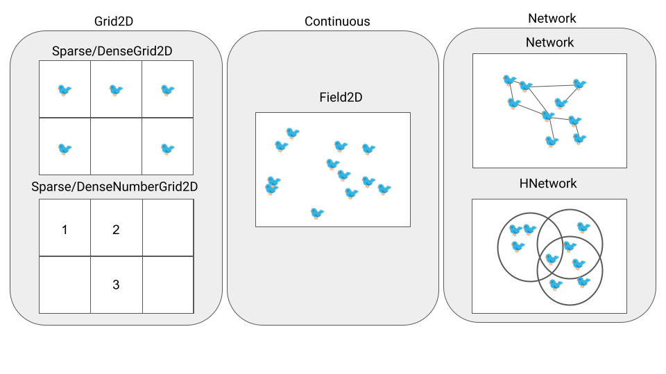
Grid2D is a data structure based on a matrix design. In a Grid2D field, agents can move across the matrix cells, and a pair of coordinates identifies their location. krABMaga exposes two types of Grid2D fields: SparseGrid2D and DenseGrid2D. SparseGrid2D is appropriate for low-density fields, where most of the cells are empty, and exploits a HashMap to speed up read and search operations. The DenseGrid2D works better for high-density fields, where most of the cells contain a value, and is based on the Rust object matrix to make write operations as fast as possible. Both fields can be further specialized in:

• an ObjectGrid2D field, namely a Grid2D field for storing any Rust structures that implements a specific set of traits. Each cell of the field may contain more than one agent.
• a NumberGrid2D, a simpler Grid2D field for placing any Rust structure that implements a specific set of traits. This field is optimized to handle primitive types, such as numerical values. In this case, each cell contains only a single agent.

This design choice lets the developer optimize their simulation performance by choosing the field that better suits the model. Field2D is a bi-dimensional (possibly toroidal) continuous space where agents can be placed anywhere within the field. The coordinates of an agent placed in a Field2D field are represented as a Real2D object consisting of a pair of floating-point values. Network is a graph-shaped field that defines non-spatial relationships between agents. This field permits the definition of directed, undirected, and weighted networks where the nodes represent agents and edges relationships between them. krABMaga also provides the HNetwork field, where the underlying interaction network is modeled as a hypergraph. Specifically, hypergraphs are a generalization of graphs in which every (hyper)edge connects an arbitrary number of nodes.

Field updates. A crucial feature of krABMaga is the use of the double-buffering technique to manage fields’ memory. Each field uses two data structures to store its values: one structure is read-only (read state), and the other is write-only (write state). At the beginning of each simulation step, the read state contains up-to-date information, while the write state is empty. Any object performing a reading (resp. writing) procedure will thus access the read (resp. write) state. Hence, the two data structures are independent, but the engine automatically synchronizes them at each step’s end. Thanks to the double-buffering technique, krABMaga can perform any read operations concurrently on the read-only data structure, thus, significantly improving the performance of the simulation. On the contrary, writing operations, which change the simulation state, are performed sequentially to avoid data race and contention on the write state.

In a nutshell, the double-buffering technique guarantees that when an agent is scheduled, the correct information (e.g., the agent’s neighbors’ location) from the previous simulation step is used.

The modeler must define how each simulation field must be updated via either one of the following functions.

1. function lazy_update(). This efficient update operation swaps the read and the write states, and it is suggested when the simulation data changes at each step. In this case, the swap approach significantly improves the performance. In practice, this function re-initializes the memory.
2. function update(). This update operation moves all the data from the write state to the read state. This function is computationally intensive and should be used when (part of) the data of the previous simulation step must be preserved.

The double-buffering mechanism of krABMaga is transparent to the modeler. Still, our framework offers additional methods that enable expert users to optimize their code for specific needs. These methods operate on the write state and are marked as unbuffered. For instance, a user may choose to design the simulation model to use the lazy_update function and, hence, obtain a more efficient execution.

Scheduler

The krABMaga scheduler manages all the discrete events happening in the simulation. In other words, it controls when the behavior of an agent (defined in the Agent.step() method) should be run. The scheduler handles the simulation timeline via a priority queue, which sorts the agents according to their scheduling time and priority. During each simulation step, the scheduler selects all agents whose scheduling time matches the current simulation time, pushes them into a helper priority queue associated with the current step (which sorts agents based on their priority), and then calls their step functions.

The modeler can access the scheduling functionalities to control the pace of the simulation through the Scheduler³ object. Specifically, krABMaga provides two functions to schedule a new agent, i.e., insert it in the priority queue:

• function schedule_once(agent, time, ordering). This function schedules a single-time agent, which will be removed from the scheduling queue after the execution of its step function. The parameters include the agent’s current step time and priority;
• function schedule_repeating(agent, time, ordering). This function schedules an agent during each next simulation step. The parameters include the agent’s current step time and priority.

The scheduler also handles the actions to perform before and after each simulation step associated with the agents (see Section 2.9) and simulation state (see Section 2.12). Further, the krABMaga scheduler can manage different types of agents within the same model.

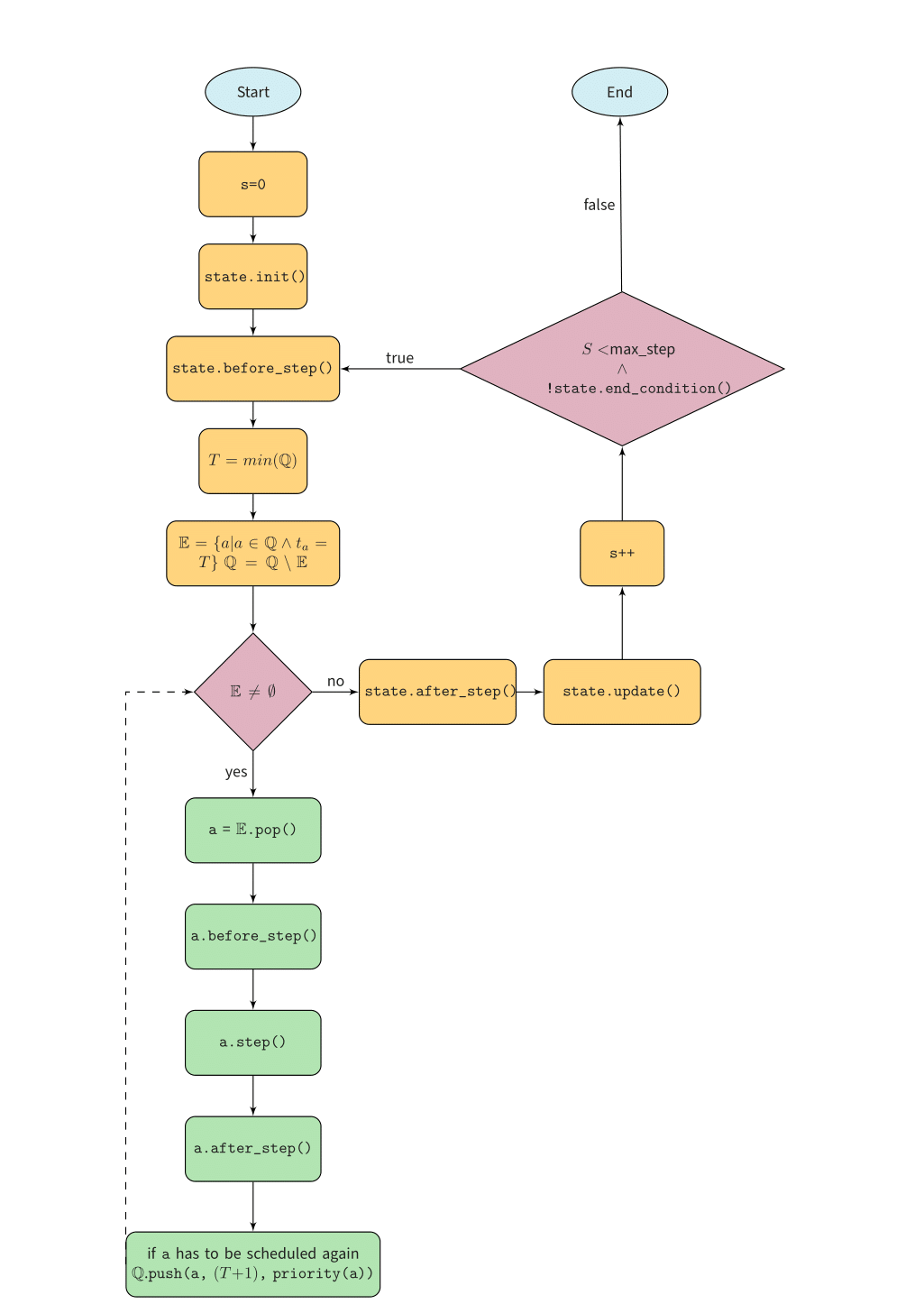
Scheduling process. The simulation process can be roughly split into three main phases. During the first phase, the scheduler initializes the number of simulation steps and its state to then invoke the state’s behavior that must be performed before the execution of each simulation step (State.before_step function). Soon after, the scheduler selects and removes from the event queue \(\mathbb{Q}\) all agents \(a\) whose scheduling time \(t_a\) matches the current simulation time \(T\) and inserts them into the priority queue \(\mathbb{E}\) associated with the current simulation step. In the second phase, the scheduler handles the execution of each agent’s behavior (Agent.before_step, Agent.step, Agent.after_step functions) contained in the queue \(\mathbb{E}\) according to their priority. The agents are pushed again in the event queue \(\mathbb{Q}\) if they need to be scheduled in the next simulation steps. When there are no more events in the queue \(\mathbb{E}\), the scheduler moves to the next phase. In the third and last phase, the scheduler invokes the state’s behavior that must be performed after the execution of each simulation step (State.after_step function) and at the end of each simulation step (State.update function) to update all the State’s data structures. The scheduler will continue processing the events until the maximum number of steps \(s\) is reached or an end condition occurs (see Section 2.12). Figure 3 summarizes the described scheduling process.

Monitoring tools

The development of an ABM is a complex process that requires the modeler to define each component properly in order to obtain an accurate simulation of the system under study. Further, ABM models usually have stochastic components, which give life to patterns that may be analysed statistically but may not be predicted precisely. For this reason, most models need to be run several times to be able to correctly analyze their behavior. To alleviate these challenges, krABMaga offers a series of declarative macros for verifying the reproducibility of a model (Zhang & Robinson 2021) and tracking simulation data. krABMaga also includes a convenient monitoring tool via a Terminal User Interface (TUI) that allows the modeler to monitor simulation events, create graphs based on tracked data, and check the simulation performance. The TUI provides some default information about the simulation, such as the step number, CPU and memory usage, and the number of steps per second executed. The user can add further information using a simple set of macro exposes by krABMaga. It is worth stressing that none of these features affect the simulation performance and execution since they are managed in a separate thread. A few details about the functions the user can manipulate to run a systematic suite of experiments and personalize the TUI follow.

• Execution-related macros
  • simulate!(state, steps, reps). This macro runs an agent-based simulation for the specified number of steps and repeats the same simulation according to the number of repetitions reps.
  • check_reproducibility!(state, steps, agent). This macro verifies whether two runs of the same simulation produce exactly the same results having fixed a common seed. The definition of the agents must implement the trait ReproducibilityEq in order to perform the reproducibility control.

• Graph-related macros
  • addplot!("Agents", "X axis", "Y axis", bool). This macro allows the modeler to create a new tab within the TUI to accommodate a new plot that can be populated using the plot!() macro. The last input parameters regulates whether the newly added plot should be stored locally in csv format.
  • plot!("Agents", "Series", x, y). This macro adds a new point of the series Series located at coordinates (x,y) to the plot Agents.
• Log-related macros
  • log!(Info, format!("STEP: {}", step)), bool). The log! macro allows the modeler to log any information within the TUI using different kinds of messages based on the event type, namely Info, Warning, Critical, and Error. An additional parameter enables saving the logs locally.

The Visualization component

An ABM framework that provides visual feedback of the simulation during its execution results in a significant advantage for the modeler by allowing a better understanding of the system behavior (Kornhauser et al. 2009). For this reason, krABMaga offers an efficient 2D visualization system based on the Bevy engine⁴, which can be run locally or in a web browser thanks to WebAssembly⁵. Moreover, our framework provides a simple control panel to manage the simulation via the egui⁶ library, which enables the user to pause, stop, and restart the simulation execution and manage its velocity (i.e., step rate). A few details about the Bevy engine and WebAssembly follow.

Bevy Engine. Rust’s combination of low-level control, excellent performance, and modern build tools makes it an exciting choice for game developers and leads to the creation of several game engines. Among these, the Bevy engine arises for its ease of use and efficiency. Bevy is a simple, open-source, data-driven game engine built in Rust that offers a complete 2D and 3D feature set. Bevy is simple to use for new developers but very flexible when used by experts providing a data-oriented modular architecture and high-performance parallelization.

WebAssembly. WebAssembly (Wasm) is a binary instruction format for stack-based virtual machines designed as a portable compilation target for any programming language that enables running applications in the browser. Wasm grants excellent performance thanks to its conversion process that does not require parsing or compiling steps to convert the source language into byte code. The result is a small executable that can run on any browser with native performance.

In krABMaga, we exploited wasm-pack⁷ to generate WebAssembly code and webpack⁸ to bundle the application for its release.

The krABMaga visualization component is entirely modular and acts as a separate system; thus, the user can either visualize the simulation or not without modifying the underlying model. This component is designed as a wrapper of the simulation model: each primary trait defined in the Engine component has its counterpart in the Visualization sub-system (e.g., the trait Agent is paired with the trait AgentRender). The Visualization component automatically manages the model initialization and the graphical update at each step.

A detailed description of the traits exposed follows.

• VisualizationState, trait used to manage the visualization elements’ startup and setup. The object implementing this trait must define how to initialize the graphics and retrieve the agent from the simulation state;
• AgentRender, trait defining how agents should be drawn. The object implementing this trait must define the sprite representing the agent in the visualization, the agent scale, location, rotation, and how the information coming from the simulation state needs to be managed to update the agent rendering;
• The Visualization component provides different traits defining how the field should be drawn based on its type:
  • BatchRender, trait designed for fields containing numerical values that have to be visualized as a simple texture. The object implementing this trait must define how the visualization engine will convert the 2D points into pixels. It is worth highlighting that the simplicity of the data structure allows the whole structure to the GPU to be sent in a single batch, hence improving overall performance;
  • RenderObjectGrid2D, trait designed for fields containing an object within each cell (not used for agents). The object implementing this trait must define how the engine will draw the object, including the sprite to use, its scale, rotation, and update method;
  • NetworkRender, trait designed for the network field. The object implementing this trait defines how the visualization engine must draw the edges.

High performance model exploration and optimization

Calibrating, exploring, and validating ABMs are crucial tasks to obtain reliable results. However, when the number of variables regulating the behavior of an ABM jumps from just a few tens to thousands or more, addressing these tasks may become computationally infeasible due to the high dimensionality of the search space.

Perrone et al. (2012) identified a community need for tools that facilitate the model exploration and optimization process. In response to this requirement, the authors developed the Simulation Automation Framework for Experiments (SAFE), which offers support from model construction to output data analysis. SAFE was designed to handle parallel execution on multi-core servers and distributed facilities.

In a similar vein, SESSL (Ewald & Uhrmacher 2014) is a Domain-Specific Language (DSL) tailored for experiments and optimization processes, functioning as a distinct layer atop simulation systems. Similarly, the nlrx package (Salecker et al. 2019) serves as an interface between R and the NetLogo framework, enabling self-contained and reproducible analysis of NetLogo models within the R language. It even allows for the utilization of high-performance computing clusters, enabling multiprocessing and the execution of large model simulations.

When it comes to high-performance computing techniques, OpenMOLE (Reuillon et al. 2013) is an example of a workflow engine specifically designed for the distributed exploration of simulation models. It provides a domain-specific language that abstracts users from the technical details required for distributing experiments in a high-performance computing environment.

krABMaga effectively meets these needs by providing model exploration and optimization APIs through the use of macros. These macros hide the complexity of the process and can be run in a parallel or distributed environment. Moreover, the framework seamlessly integrates with cloud computing platforms, employing the Function-as-a-Service (FaaS) model. In particular, the parallel mode leverages the Rayon library⁹, enabling data parallelism, while the distributed mode harnesses the MPI (Message Passing Interface) protocol via the rsmpi crate¹⁰, a Rust-based MPI binding. Additionally, krABMaga extends support to the Amazon AWS platform¹¹, facilitating the embedding of simulation execution within an independent function that can be deployed and run in parallel on the cloud.

Here, we describe the krABMaga’s model exploration and optimization macros in their sequential version. Each macro is also configurable to exploit different computing back-ends by specifying the optional enum parameter ComputingMode, which can assume the values parallel, distributed, or cloud. By default, each macro is run sequentially in the local environment.

For further details, we refer the reader to the official krABMaga documentation¹².

Model exploration

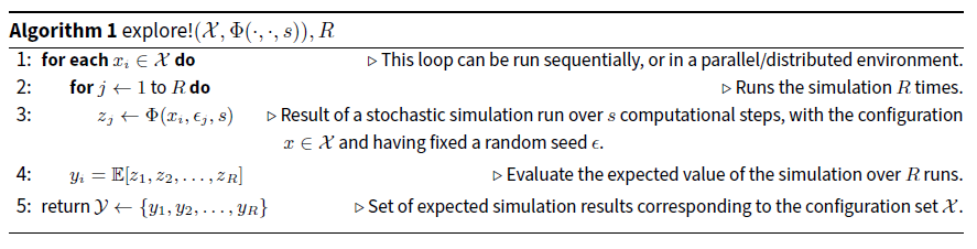
This process, aka parameters sweeping, consists in analyzing the model sensitiveness by varying the input configurations. Algorithm 1 reports the pseudo-code of the procedure. For each input configuration \(x_i \in \mathcal{X}\) (Line \(1\)), the framework runs the simulation \(\Phi\) over \(s\) computational steps, with a fixed random seed \(\epsilon_j\). This process is repeated \(R\) times (Lines \(2-3\)). The procedure returns the expected simulation values obtained from each input configuration (Lines \(4-5\)).

krABMaga supports the user in generating random values for an input parameter by exposing the macro
gen_param!(type, min, max, n), which returns a vector of \(n\) uniformly distributed input values in the range min and max. Further, the framework provides the output data \(\mathcal{Y}\) within a DataFrame structure, which permits a straightforward analysis of the results and can be easily exported as a CSV data file.

krABMaga supports the user in generating random values for an input parameter by exposing the macro
gen_param!(type, min, max, n), which returns a vector of \(n\) uniformly distributed input values in the range min and max. We chose to implement uniform distributions as our first method, given their widespread use in simulation scenarios. We plan to incorporate additional distributions for creating random parameters in future updates. Furthermore, the framework provides the output data \(\mathcal{Y}\) within a DataFrame structure, which permits a straightforward analysis of the results and can easily be exported as a CSV data file.

Model optimization

This process, aka simulation via optimization, exploits a search-based optimization algorithm for finding the best input configuration for the simulation. In krABMaga, we implemented three parameter optimization approaches, accessible via as many Rust macros.

Random search[random_search!(...)] explores the parameter space by using a random searching algorithm, which consists of iteratively computing and evaluating a set of random input configurations until the maximum number of iterations is reached or a desired simulation score/error is achieved.

Evolutionary search[evolutionary_search!(...)] optimizes the simulation parameters by adopting an evolutionary searching strategy. Specifically, krABMaga provides a genetic algorithm-based approach (Stonedahl & Wilensky 2011).

Bayesian search[bayesian_search!(...)] performs a Bayesian optimization-based searching strategy (Jones et al. 1998) for parameter optimization similarly to the evolutionary strategy.

In krABMaga, each of the above macros implements a modified version of Algorithm 1. Specifically, each strategy defines how the set of input configurations \(\mathcal{X}\) is defined; then, a goodness or error value is evaluated for each set of expected simulation results to iteratively inform the parameter search space strategy.

Programming with krABMaga: the Wolf, Sheep, and Grass Model

This Section describes the process of designing and implementing an ABM with krABMaga, using the Wolf, Sheep, and Grass (WSG) model as a use case. This model is a typical example of the effective use of ABMs and has been widely studied (Wilensky & Reisman 1998, 2006).

Defining the WSG model

WSG is a model which simulates the population dynamics of predators and prey that coexist in a shared ecosystem. Wolves are the predators eating sheep, their prey, which, in turn, eat the grass. Both wolves and sheep consume energy for each activity; so, food availability dictates the ability to restore energy and survive. Specifically, sheep survival depends on the grass growth rate. If the number of sheep is too high, grass will not grow in time to be eatable. Wolves’ survival relies on sheep’s reproduction rate. If the wolves’ number is too high, they will eat too many sheep, precluding their reproduction.

Given its dynamics, the WSG model requires a set of parameters correctly calibrated to realize a stable system. A system is called stable if the agents’ population fluctuates over time but never reaches extinction. Conversely, the system is unstable if all the agents die at any given point.

WSG agents

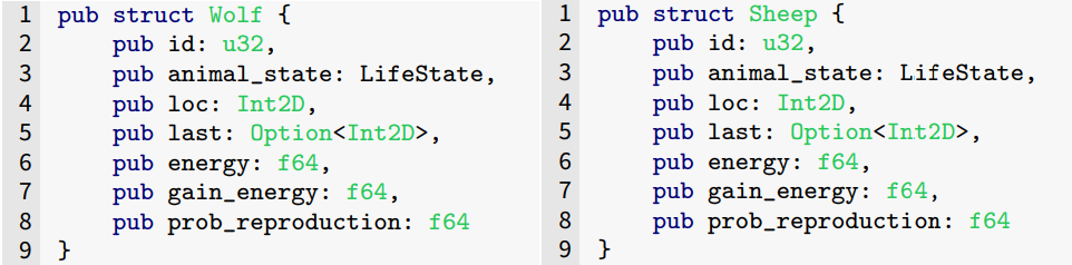
The WSG model has three fundamental concepts: wolves, sheep, and grass. Wolves and sheep move and actively interact with the environment, while the grass is stationary and only grows over time. For this reason, wolves and sheep can be represented as agents, while the grass as a numerical value (see Section 3.12). Despite wolves and sheep acting similarly, their interaction with the system is different; thus, these two entities are modeled as separated agents. Regardless of their nature, both agents need to carry some essential information: a unique identifier (id), their current location in the field, and their previous location. Additionally, the WSG model needs specific properties for each agent, such as (i) its current energy, (ii) the energy gained from food, (iii) its reproduction probability, and (iv) its life state: dead or alive. The definition of the Wolf and Sheep agents is illustrated in Figure 4.

In krABMaga, each entity representing an agent must implement the trait Agent and define its behavior in the function step(). Wolves and sheep perform three actions: moving, eating, and reproducing.

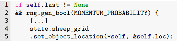
Moving. Wolves and sheep randomly move around the landscape. With a given probability \(\alpha\) (momentum_probability), the agent moves in the same direction as the previous step; with probability \(1-\alpha\), the agent moves in a random position. Figure 5 depicts the code regulating how sheep move, but the same applies for wolves on the wolf_grid (see Section 3.12).

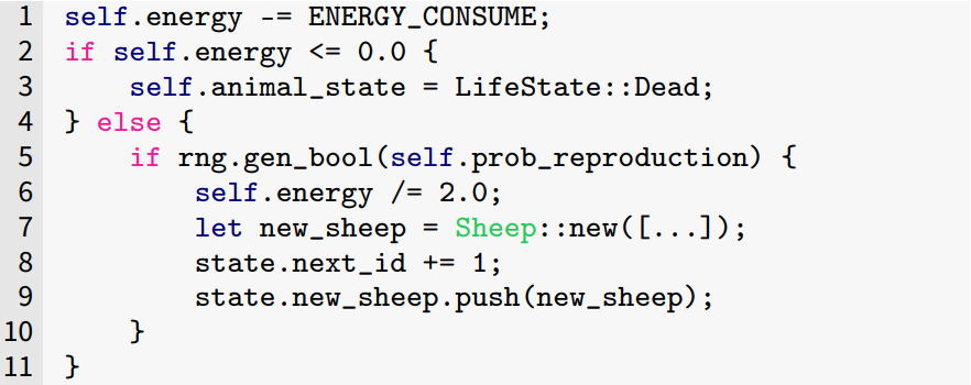
Survival and Reproduction. After moving, wolves and sheep simulate energy loss by subtracting a fixed value from their energy. If their energy drops below zero, the agent sets its LifeState to Dead. If the agent survives, it tries to reproduce. If it succeeds, it halves its energy and creates a new agent. It is worth noting that agents cannot add new entities to the scheduler within their function step() as only the simulation State object can interact with the scheduler. The new_sheep and new_wolves arrays of the simulation State serve this purpose. Figure 6 depicts the code for the sheep agents, but the same applies for wolves using Wolf::new().

Eating. The system’s stability depends on the possibility of wolves and sheep eating. After moving to a new location, agents will search for food and eat if certain conditions are met. The implementation of eating behavior differs between wolves and sheep due to the different natures of their food, as wolves eat other agents (sheep) while sheep eat a simpler entity (grass).

Eating grass. A sheep can eat grass on its location if it is fully grown and the grass has not been eaten by another sheep in that step. This last requirement is verified using the function get_value_unbuffered() that accesses the write state of the grass field. If the value obtained is not null, another sheep has already eaten the grass since it has been written in the write state structure. If the sheep successfully eats the grass, it sets the grass value on the field to 0 and gains some energy, as depicted in Figure 7.

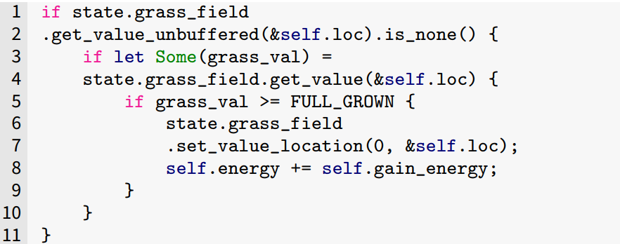
It is crucial to stress that using the function get_value_unbuffered() allows access to up-to-date information since the updates of the data structures only happen at the end of the simulation step. This approach guarantees that if a sheep eats some grass in a location during a given step and, later on, but in the same step, another sheep moves in the same location, it will correctly see the grass level equal to zero.

Eating sheep. A wolf can only eat a sheep on its location if another wolf has not already eaten the prey in that step. This requirement is checked using a dedicated data structure storing eaten sheep (see Figure 8). Wolf agents can modify the simulation field since their function step() has access to the state of the simulation. However, no agent can manipulate the scheduler due to the krABMaga safety policy. To overcome this limitation, we followed the same strategy used when introducing new agents: we added the array killed_sheep in the simulation State object to remove the eaten sheep from the scheduler.

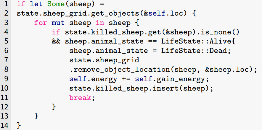
When a wolf eats a sheep, it sets the LifeState of its prey to Dead, removes the agent from the field, inserts it in the killed_sheep array, and gains some energy. Figure 8 shows the logic of this process.

WSG state

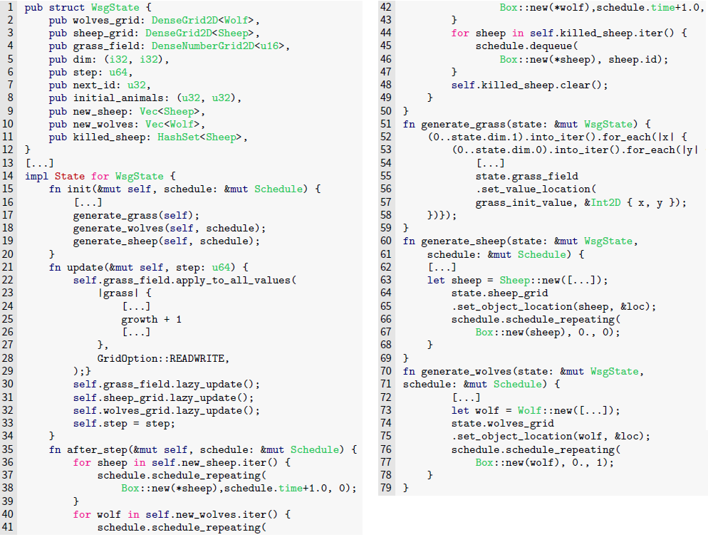
In krABMaga, the simulation State object, which implements the trait State, initializes the model, defines and updates the data structures regulating the model’s logic, schedules the agents, and controls the pace of the simulation. In this example, the WsgState object defines the (i) simulation fields, (ii) their size, (iii) the current simulation step, (iv) a unique id counter to assign different identifiers to new agents, (v) the number of agents, i.e., sheep and wolves, and (vi) three data structures to support the addition to and removal from the scheduler of agents (see Section 3.3). More specifically, the WsgState object initializes three different fields to manage the three entities of the model: the grass, wolf, and sheep fields. Specifically, the grass field is instantiated as a NumberGrid2D field, where each cell contains a numerical value representing the grass growth state, while the wolf and sheep fields are instantiated as two DenseObjectGrid2D structures. Using two different fields to handle the behavior of wolves and sheep improves the overall performance of the simulation when looking for a specific kind of agent; for instance, if a wolf tries to eat a sheep, the only structure queried will be the sheep field. Lines \(1-12\) of Figure 9 list the above properties.

Initialization phase. The initialization of the simulation happens in the function init() (Lines \(15-20\)). This function populates the three simulation fields by adding grass values, sheep, and wolves. Specifically, the method generate_grass() iterates through the grass_field cells and inserts a value representing the grass available in each cell (Lines \(51-59\)). The methods generate_sheep() (Lines \(60-69\)) and generate_wolves() (Lines \(70-79\)) work similarly: they create the respective agent, place it in a given location the corresponding fields, and add it to the scheduler’s queue via the function schedule_repeating(), which notifies the scheduler that the agents need to be scheduled in all following simulation steps. Here, we emphasize the use of the Box structure, which wraps the newly created agent (either a wolf or a sheep) and enables krABMaga to handle multi-agent simulations.

Updating phase. The WsgState object handles the update of all fields during each simulation step through the definition of the mandatory method update(). In particular, this method also implements the grass-growing process (Lines \(22-29\)), which increases the grass values of all cells in the grass_field via the function apply_to _all_values. The parameter GridOption::READWRITE ensures that the existing information is not overwritten. In more detail, this option allows us to check the WriteState structure before increasing the grass values since a sheep agent could have already written that field’s cell (i.e., eating all grass). In Lines \(30-33\), all simulation fields are updated.

In this use case, the State object also implements the method after_step that defines the logic regulating the eating and reproducing behavior of the agents (Lines \(35-50\)). After each step, the WsgState object iterates through the new_sheep and new_wolves structures to add agents in the scheduler using the method schedule_repeating() while it iterates over the array killed_sheep to remove dead agents from the scheduling process via the method dequeue().

Running and analyzing the WSG model

At this point, we have defined all elements of the WSG model. Now, let’s see how to run it and analyze its execution with the TUI.

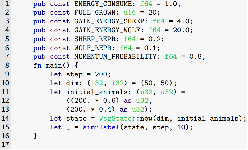
Running the simulation. The WSG model includes several parameters influencing the system’s evolution and stability, such as the number of sheep and wolves, the cost of each agent’s step, the energy gained from food, and the grass growth rate. Figure 10 shows the main.rs file, which defines these parameters (Lines \(1-7\)). Here, the function main() instantiates the simulation State with the required parameters and runs the macro simulate! to launch the simulation.

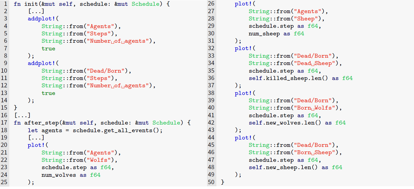
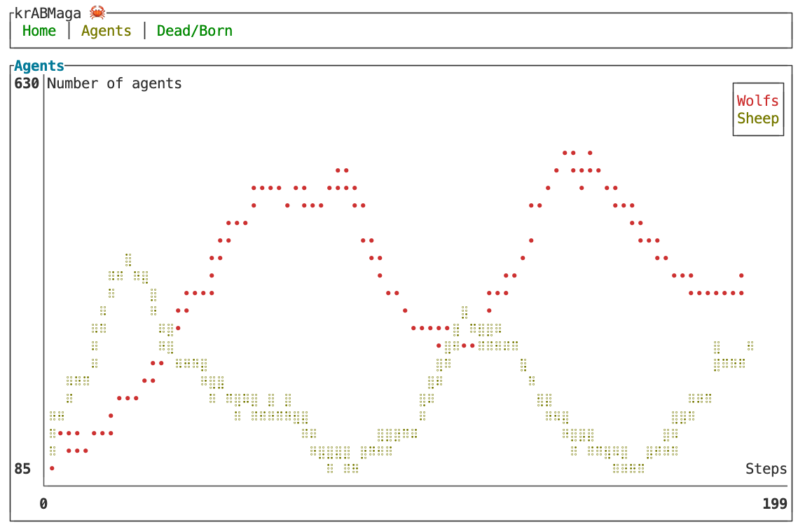
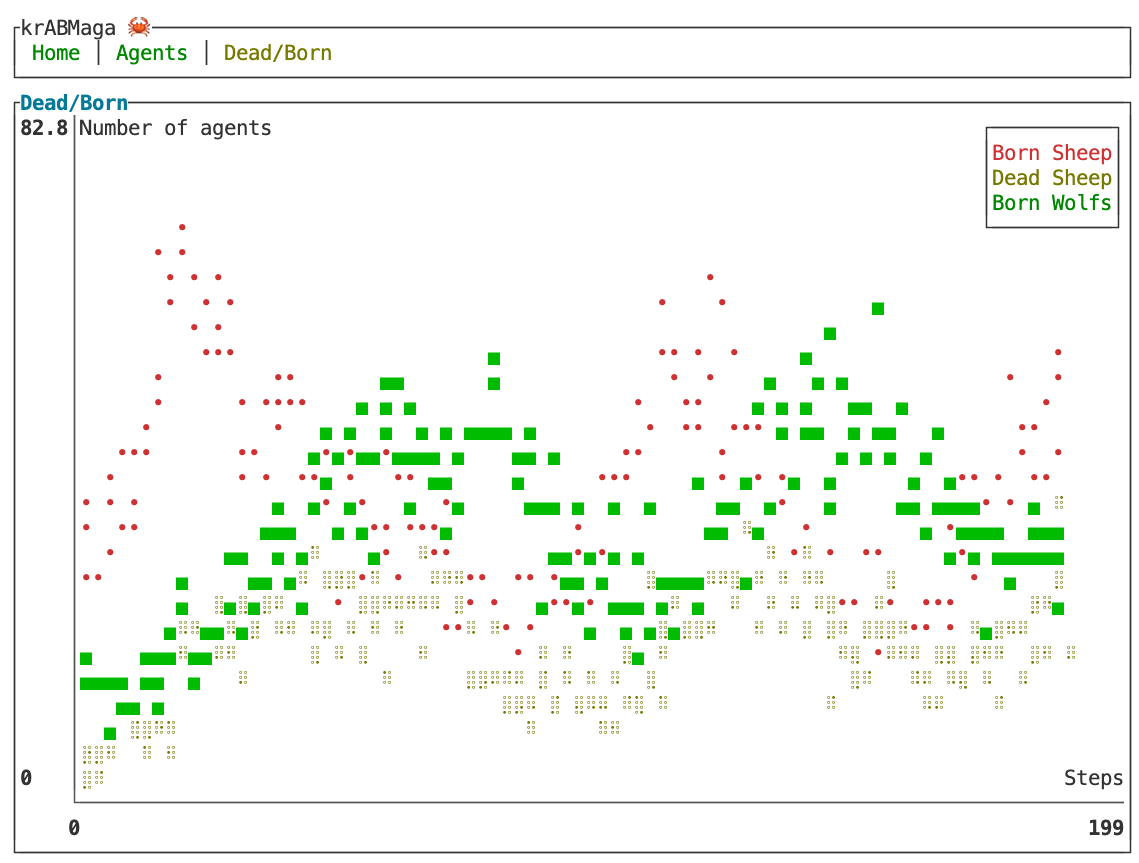
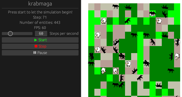
Analyzing the simulation. The krABMaga GUI terminal helps us investigate the stability of the ecosystem predator/prey by creating dynamic plots of the simulation status. These plots are managed within the State object and, hence, have access to all simulation data (see Figure 11). The structure of each plot is defined within the function init() via the macro add_plot!(), which specifies the plot’s title and labels (Lines \(3-14\)). Then, the plot is populated using the macro plot!() called within the function after_step(), which adds a data point after each simulation step (Lines \(20-49\)). The code listed in Figure 11 results in two plots: the first shows the trend of the wolf and sheep population (see Figure 12), while the second tracks newly born wolf and sheep agents, as well as the number of sheep killed by wolves (see Figure 13).

Visualizing the WSG model

After having the WSG simulation up and running, we can use the Visualization component of krABMaga to visually monitor the behavior of the developed model. The trait VisualizationState manages the entire visualization model similar to the trait State in the sense that we need to initialize (function on_init()) and update (function update()) the visualization of the grass field and the agents. The function get_agent_render() fetches the data structures defined in the model (grass_field, wolves_grid, sheep_grid).

In this specific use case, wolf and sheep agents move in the space, while the grass is a static environmental element. To render the agents’ movement, we let the Wolf and Sheep objects implement the trait AgentRender. Then, we defined how the engine must draw the agent at each step, specifying its position, orientation, and scale in the function update(). The only difference between sheep and wolf agents resides in their representing sprites, specified in the sprite() function. Eaten sheep disappear from the field. In the method before_render(), run before each simulation step, we inform the visualization to render the newly born agents. To graphically represent the growing grass, we implemented the trait BatchRender in the field DenseNumberGrid2D. In more detail, we used the method get_pixel() to specify the color of each cell based on the amount of grass contained (the greener the cell, the higher the grass available).

To actually use the visualization component, we need to define a Visualization object within the function main(), which allows us to set up the graphical properties of the visualization and run it.

A snapshot of the visualization of the WSG model is depicted in Figure 14. The complete code is available on the krABMaga repository¹³

Related Work

The interest of the research community in ABMs has considerably increased recently thanks to the numerous and various application fields to which the agent paradigm brings considerable advantages. In light of this surge of interest, several tools and frameworks have emerged to facilitate the development, execution, and analysis of ABMs, addressing the needs of different communities of experts. For instance, some platforms, such as MASON and Repast, are close to the computer science world, providing general-purpose libraries and frameworks usable with common programming languages like Java. Other tools, like Netlogo, furnish simplified language specifically designed to make ABM development accessible to non-experts developers instead. In this Section, we outline some of the most important and impactful frameworks for developing and running ABMs to offer the reader an overview of existing literature and, hence contextualize the significance of krABMaga. Here, we focus on general-purpose ABM software used for real applications, with a stable and maintained software version, consistent user base, and associated research works and projects. A more comprehensive survey about ABM tools and software is described in Abar et al. (2017).

Here, we begin our overview with MASON (Luke et al. 2005) since its architecture profoundly inspired krABMaga development. MASON is an open-source discrete-event simulation toolkit in Java designed to be a general-purpose tool usable for the design, execution, and visualization of ABMs. MASON provides the developer with functionalities and APIs supporting the most common needs of a modeler, including the definition of common agents’ behaviors, environment creation with different fields, and scheduling management. One of MASON’s main advantages is its snapshot system which enables the user to stop and save a simulation to later resuming it on another machine, thanks to the compatibility of the Java Virtual Machine. Moreover, additional features are available in MASON thanks to the existing extension, including the use of GIS data with GeoMASON (Sullivan et al. 2010), model exploration with ECJ (White 2012), as well as the possibility of running a simulation on distributed and cloud systems with DistributedMASON (Cordasco et al. 2018).

Agents.jl (Datseris et al. 2022) is a recent framework for agent-based simulations that provides utilities and ad-hoc structures for implementing, running, and visualizing models exploiting the Julia programming language. Agents.jl focuses on performance and ease of use, allowing users to develop models with only a few lines of code. The framework is available as a Julia library and is easily usable with the plethora of analytical tools of the Julia ecosystem. Agents.jl offers the most commonly used fields, like grids, continuous space, and graphs, and supports the use of OpenStreetMap data. This library also provides model exploration functionalities and parallel and distributed computation support.

From research that exploit the accessibility of a programming language to provide a usable ABM framework, Mesa (Kazil et al. 2020) is one of the most used and actively supported. Mesa is an open-source modular framework for building, analyzing, and visualizing ABMs built upon Python to provide usability and accessibility. The architecture of Mesa is composed of three major elements: model, analysis, and visualization. The model component exposes all the methods to define the agent behavior and the simulation environment. The analysis functionalities include recording, storing, and exporting data from the model. Finally, the visualization component provides a front-end browser-based visualization to design, interact with, and control the model. The main advantage of Mesa resides in its extensibility; the community is, therefore, encouraged to create several extensions to handle, for instance, multi-processor systems or GIS data.

The field of ABM simulations is constantly expanding with new software and tools. However, some works represent the pillars of ABM development. Besides MASON, NetLogo (Wilensky 1999), Repast (North et al. 2013), Flame (Holcombe et al. 2006), and AnyLogic (Borshchev et al. 2002) are the most relevant and used tools for simulation design.

NetLogo is a free agent-based modeling environment implemented in Java/Scala that has become the standard platform for developing ABMs. NetLogo is a robust, powerful, simple-to-learn, and easy-to-use Domain-Specific Language offering a GUI to create and edit components to realize any simulation. The importance and popularity of NetLogo has risen thanks to its community which is constantly providing extensions to enrich NetLogo with new functionalities. Examples of such extensions include GIS data, 3D visualization, and integration with other languages, like Python with PyNetLogo (Jaxa-Rozen & Kwakkel 2018) or Pylogo (Abbott. & Lim. 2021), or R with RNetLogo (Thiele 2014). Other relevant extensions worth to be mentioned are HubNet (Jiang & Zhao 2009) and BehaviorSpace (Railsback et al. 2017). HubNet allows the creation of a participatory simulation over a network where users can control and interact with a simulation running on a remote machine. BehaviorSpace includes parameter sweeping capabilities that enable data collection from multiple executions and the exploitation of distributed and parallel techniques.

Repast is an open-source family of widely used agent-based modeling and simulation platforms, implemented in several programming languages, which include many built-in features for ABM development. Repast Simphony (North et al. 2013) is a Java-based modeling system based on a modular plug-in architecture that allows users to replace specific components. This toolkit provides automated methods to perform all the common tasks required in a simulation and supports model visualization in 2D and 3D, GIS Data, a snapshot system, and the capability to run multi-threaded simulations. Further, the Repast Simphony plug-in enables adding a wide range of external tools for any needs, like statistical analysis, data mining, or integration with other languages.

RepastHPC (Collier & North 2013) is a parallel and distributed C++ implementation of Repast Simphony specific for ABM simulation targeting large-scale distributed computing platforms based on MPI. The newest member of the Repast suite is Repast4Py (Collier et al. 2020), a Python-based framework based on RepastHPC to develop distributed ABMs.

FLAME is a generic agent-based modeling system that provides a formal framework for creating models compatible with any computing platform. The framework is inherently parallel and can automatically optimize performance without user effort. Users can describe a model using the XXML language based on state machines that FLAME will then compile into a C-based application. FLAMEGPU (Richmond & Chimeh 2017) extends FLAME to easily use GPU capabilities without deep knowledge of the CUDA programming language or optimization strategies. Specifically, FLAMEGPU maps the formal XXML specification used in FLAME to the CUDA programming language to produce a parallel and efficient application.

We conclude this overview with AnyLogic, proprietary software for developing ABMs through a simple user interface, hence, particularly suitable for non-expert developers. The AnyLogic platform includes APIs for modeling agents’ behavior, supporting several environments (e.g., GIS space), and different execution paradigms (e.g., distributed and parallel computation). AnyLogic offers visualization capabilities and a GUI to control any aspect of the simulation during its execution visually. Moreover, a snapshot system allows the user to stop and restore the simulation later. AnyLogic Cloud is an extension of the main platform that permits running ABMs on cloud computing resources.

Table 1 summarizes the ABM frameworks and tools described, emphasizing whether they provide support for the most relevant features. The last two rows of the table show the declared efficiency and ease of use for each tool as discussed in the survey by Antelmi et al. (2023). Specifically, the term ease of use refers to the effort required for installation and setup procedures, the presence of examples, and the clarity of the documentation provided. The ease of use of a tool is closely tied to the programming language used (higher-level languages are generally easier to approach), the number of available functionalities (the higher, the better), and the availability of a dedicated GUI or a VSL (which can further reduce the need for coding). The term efficiency refers to the capability of the ABM tool to handle large and complex models granting low execution time. The classification of ABM tools according to their efficiency is determined by how the authors position themselves within the state-of-the-art regarding the potential to handle large-scale models and the efficiency in executing them.

Table 1:Comparison of ABM framework/software features.

ABM Tool / Features	MASON (Luke et al. 2005)	Agents.jl (Datseris et al. 2022)	Mesa (Kazil et al. 2020)	NetLogo (Wilensky 1999)	Repast (North et al. 2013)	Flame (Holcombe et al. 2006)	AnyLogic (Borshchev et al. 2002)	krABMaga
Programming Language	Java	Julia	Python	Java and Scala, Python and R with extensions	C++, Java, and Python, based on version	C and XXML	Java	Rust
Supported environment fields			Grid, Continuous space, Network
Visualization	2D/3D	2D/3D	2D/3D with extension	2D/3D	2D/3D	3D	2D/3D	2D (3D Experimental)
GUI	Yes, limited	No	Yes, limited	Yes	Yes	No	Yes	Yes, limited
GIS Data	Yes, with extension	No	Yes, with extension	Yes	Yes	No	Yes	No (Ongoing)
Model Exploration	Yes, with extension	Yes	Yes, with extension	Yes, with extension	Yes, with Repast Simphony	No	Yes	Yes, parallel, distributed and cloud computing are also supported
Checkpoint and Snapshot	Yes	No	No	Yes	Yes	No	Yes	No (Future Work)
Parallel In-Model Execution	No	No, delegated to the modeler	Yes, with extension	No	Yes, with Repast HPC	Yes	Yes	Yes, Experimental
Distributed In-Model Execution	Yes, with Distributed MASON	No, delegated to the modeler	No	Yes, with extension	Yes	Yes	Yes	Yes, Experimental
Declared efficiency	High	High	Low	Very low	Medium	Medium	High	High
Declared ease of use	Medium	Medium	High	Very high	Medium	Medium	Very high	Medium

Current state-of-the-art regarding ABM software includes tools more focused on ease of use, like NetLogo and Mesa, or frameworks more centered on performance and flexibility, like MASON and Repast. With krABMaga, we tried to cover the current open challenges in the ABM field, aiming to provide a valuable tool that can offer good performance and reliable executions while still granting an accessible development experience. To this end, we provide extensive documentation, examples, and functionalities to abstract the ABM development process from the engine-related mechanisms and the specific nuances of the Rust programming language. While a basic familiarity with Rust is beneficial, it is noteworthy to highlight that it is not a prerequisite for using our framework, even though some coding skills are needed. Many implementation details remain transparent to the user, allowing individuals without extensive Rust expertise to utilize our tool effectively.

Performance Evaluation

This Section presents a two-fold performance evaluation of krABMaga: first, we investigated the library’s efficiency in running different ABM simulations against the most adopted ABM tools, then we evaluated the scalability potential of the model optimization module.

Model simulation experiment

In this experiment, we are interested in showing the performance of krABMaga in running ABM models and comparing it with the most representative ABM tools, namely Agents.jl, MASON, Mesa, NetLogo and Repast.

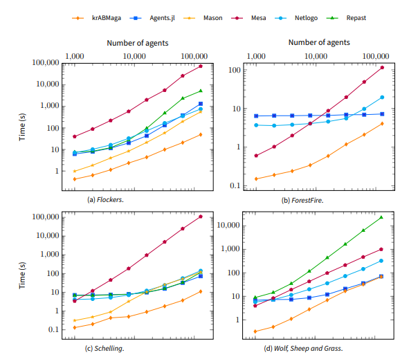
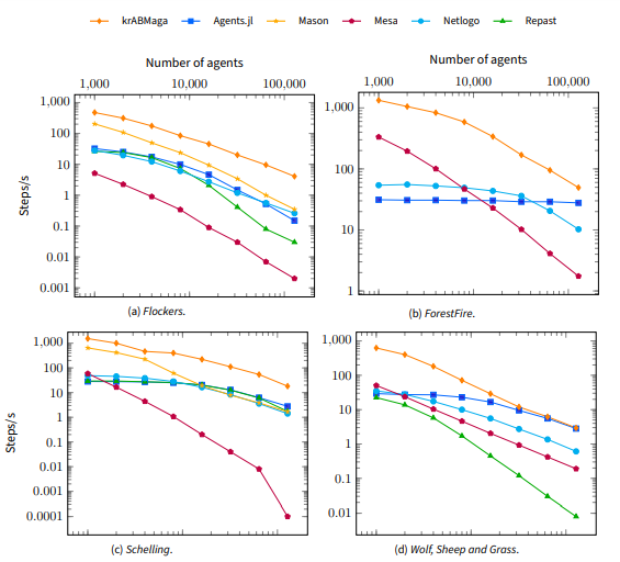
Models. As a benchmark, we employed the following ABMs, each with its peculiarities regarding data structures, agents’ behaviors, and environment types.

• Flockers. Developed by Craig Reynolds, this is one of the most famous ABM simulating a flock’s flying behavior. In this model, the agents move within a continuous toroidal space according to a simple set of rules.
• Schelling. This is a simple segregation model based on a 2D grid in which agents decide whether to move into a new cell based on the status of their neighbors.
• Wolf, Sheep and Grass. This multi-agent model simulates the population dynamics of predators and prey coexisting in a shared environment.
• ForestFire. This stochastic spreading model is realized as a cellular automaton to reproduce the fire diffusion in a forest.

To perform a fair comparison, we benchmarked only official released model for each platforms; still, some differences could exist due to the variance in the frameworks, mainly because of the different programming languages involved. The model and benchmark implementations are available on the krABMaga repository¹⁴

Benchmark configurations.All experiments have been performed on the same virtual machine running over a VMware Esxi hypervisor and equipped with: Ubuntu 21.10 x86_64 machine, 8 VCPU, 16GB RAM, and 256 storage (on SDD). The performance of each framework has been tested with different models configurations, starting with a field of size \(100\times100\), \(1000\) agents, and \(200\) steps, while keeping an agent density of \(\cong 10 \%\), calculated as \(\frac{\text{width} * \text{height}}{\text{number of agents}}\). We obtained the other configurations by doubling the number of agents and changing the field dimension to preserve the agent density:

1. Agents: \(1000\) - Field size: \(100\times100\)
2. Agents: \(2000\) - Field size: \(141\times141\)
3. Agents: \(4000\) - Field size: \(200\times200\)
4. Agents: \(8000\) - Field size: \(282\times282\)
5. Agents: \(16000\) - Field size: \(400\times400\)
6. Agents: \(32000\) - Field size: \(565\times565\)
7. Agents: \(64000\) - Field size: \(800\times800\)
8. Agents: \(128000\) - Field size: \(1131\times1131\)

Each experiment has been run \(10\) times.

Results. Figure 15 shows the results of our experiments, focusing on each framework’s average running time (in seconds) when varying the model dimension while keeping the agent density fixed. Such values only keep into account the actual simulation time and exclude the initialization time required by each engine. Overall, krABMaga always performs better than the other platforms, requiring the lowest computational time regardless of the computational load. In only a single scenario, Agents.jl reached the same performance as our platform (see Figure 16d) but consumed up to the \(90\%\) of the system’s available memory. Figure 16 refers to the same benchmark, reporting the average number of simulation steps per second. In general, the heavy memory usage of some platforms limited the maximum computational workload tested, as these platforms were unable to simulate larger systems. For that reason, we were unable to assess configurations with a higher computational complexity. It is important to stress that these results come from adequately using different fields, data structures, and methods in each framework since every model exposes different peculiarities that must be appropriately addressed when implementing the corresponding ABM.

Model calibration experiment

In this second experiment, we analyzed the scalability of krABMaga when calibrating an ABM via the model optimization functionality offered by our simulation engine. The full code of this experiment is available on the official krABMaga example repository.¹⁵.

Model. As a benchmark model, we built an ABM for simulating an epidemic spreading in a population, where agents can get infected via their neighbors in a similar fashion of the work of Crooks & Hailegiorgis (2014). Specifically, we implemented the Susceptible (S), Infectious (I), Recovered (R) compartmental model, which specifies how agents move from the state \(S\) to \(I\) (i.e., become infected with a probability \(\beta\) proportional to the number of infected neighbors), and from \(I\) to \(R\) (i.e., recover from the infection with a probability \(\gamma\)). The agent contact network follows the Barabási-Albert preferential attachment rule. Some details about the simulation follow.

The simulation State, in addition to the network structure, includes the definition of the parameters governing the dynamics of virus spread: (i) the probability that a susceptible node transitions to an infected state, and (ii) the probability that an infected node transitions to a resistant state. The simulation begins with the network containing only one infected node randomly placed within it and continues until either the maximum number of steps is reached, or there are no more infected nodes. Each step corresponds to a day, during which nodes may alter their status. Specifically, susceptible nodes examine the status of their neighbors, and if any neighbor is infected, there’s a chance that the susceptible node becomes infected as well. Infected nodes, on the other hand, make an attempt to recover during each step, changing their status to resistant. In contrast, resistant nodes remain inactive since they are immune to infection and cannot infect others.

This sample scenario particularly fits the ABM simulations that krABMaga intends to support. Fitting an epidemic model with actual data and then performing experiments on top of the designed model usually requires (i) exploring the parameter space to calibrate the model’s input parameters, (ii) verifying the model’s correctness, (iii) validating the model’s output, (iv) analyze the sensitivity of the model, and finally (v) run the intended experiments. Since each phase requires running the simulation multiple times, guaranteeing that each run is efficient and reliable is critical. For simplicity, we will only focus on the first listed phase in this use case

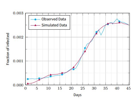
Calibration data. As ground-truth data, we used the Italy’s average number of daily new infections during the SARS-CoV-2 virus pandemic (moving average over seven days). In particular, we focused on a period of \(45\) days from December 2021 to January 2022, when the Omicron variant caused a new outbreak. This dataset is available on the official website of the Istituto Superiore di Sanità, the leading public health body in Italy¹⁶. Models of the like are widely described in the literature (Clara & Liu 2020; Hoertel et al. 2020).

Simulation setting. We simulated \(10,000\) agents for \(51\) days (three days more than the calibration time window to compute the average of new simulated infections). We normalized the infection data by the size of the Italian population (divided by \(60\)M).

Optimization strategy. To find the input parameter configuration generating outputs that best fit real-world data, we used the evolutionary search approach offered by krABMaga. In more detail, we considered an initial population of \(128\) randomly generated individuals, \(20\) simulation repetitions for evaluating a single configuration (e.g., individual), and \(2000\) optimization loops (e.g., generations). Specifically, each individual comprised two real value genes, representing the infection and recovery probabilities [\(\beta\), \(\gamma\)]. At each generation, the evolutionary strategy computed the new population by selecting the best \(20\)% of individuals and generating the remaining \(80\)% using a crossover operation (combining two random individuals from the previous generations). A mutation operator was then applied to change one of the two genes of the individuals randomly. The simulation output represented the average error between simulated and real data.

The overall calibration process resulted in about 5 million simulation executions. If all these simulations were carried out sequentially, it would have taken approximately 172 days (this estimate derives from summing the running time of each simulation execution). However, we completed the task in just 45 hours by leveraging distributed computing.

Results. Figure 17 shows the infection curves derived from simulated data based on the best configuration computed by the optimization process and the real infection curve. Table 2 focuses on some statistics comparing a sequential execution of the optimization process against its parallel/distributed version. We performed this comparison on a virtual cluster machine of \(16\) nodes running over Amazon AWS EC2, where each node used the c4.2xlarge instance type and was equipped with an Intel Xeon Processor with \(8\) virtual CPUs, \(15\) GB of memory, and a high-speed network. We analyzed the system’s performance by running the optimization process for one hour and by varying the number of VCPUs and incrementing the number of nodes. We collected the number of computed generations per hour (Gs/h), the time (seconds) for computing a generation (s/G), and the speedup against the sequential execution for each setting. As highlighted in the table, the best performance is achieved in the last distributed setting using \(16\) nodes and \(128\) VCPU, which is \(96\) times faster than the sequential setting. It is worth noting that we only report the simulation speedup to stress krABMaga’s capabilities in scaling up in such scenarios. Given the results from the previous experiment (showing that krABMaga achieves the lowest simulation time when varying the workload), we did not replicate this scenario using other simulation engines.

Table 2:Evaluation of krABMaga’s scalability on an Amazon EC2 virtual cluster machine.

Backend	#Instances	VCPUs	Gs/h	s/G	Speedup
Sequential	1	1	0	7459	1
Parallel	1	8	3.1	1149	6.5
Distributed	2	16	6.2	579	12.9
Distributed	4	32	12.1	297	25.1
Distributed	8	64	23.2	155	48
Distributed	16	128	44.3	81	92

Conclusion and Future Work

ABMs are a powerful approach to unraveling the complexity governing real-world systems. Over the last decade, the need for more elaborate computing-demanding models gave rise to many frameworks and tools to run ABM simulations. The mostly adopted ABM frameworks either focus on the easiness of use by non-expert users, computational efficiency, which requires technical skills, or a trade-off between these two elements. However, scalability and efficiency become critical requirements even when small-scale ABMs need huge computational support. In such cases, having a simulation engine able to strongly improve the running times of a single simulation is the only viable option to enhance the overall ABM model development’s performance without (or only partially) introducing new computational resources. At the same time, guaranteeing the absence of any memory flaws that could invalidate the whole experiment is another fundamental condition.

To address the requirements of simultaneously offering efficiency, reliability, and safeness, we presented krABMaga, a modern open-source library for agent-based modeling and simulation written in Safe Rust. Our library offers native support for reliable and efficient long-running ABM simulations. In this paper, we described the architecture of our simulation engine, discussing its main characteristics and functionalities, such as the support for high-performance model exploration and optimization for ABM. The performance evaluation of krABMaga against the most used open-source ABM software demonstrated how our framework could provide optimal performance regardless of the computational load. Our experiments also proved the scalability of krABMaga, thus, its potential in handling large-scale models.

We plan to continue the development of krABMaga along two main directions to build a more comprehensive tool over time. The first direction aims to improve the system’s modeling capabilities by introducing the support for (i) 3D simulations (which consists of adapting the current solution of 2D fields in the 3D space and extending the visualization component to support these fields); (ii) in-model parallelization, and (iii) the integration of GIS data (whose visualization with the Bevy engine requires significant effort since it does not offer native support). The second direction focuses on enhancing krABMaga’s support to all ABM model developing phases, including calibration, verification, validation, sensitivity analysis, and experimentation, to fully assist the developer by making these phases as transparent as possible.

References

ABAR, S., Theodoropoulos, G. K., Lemarinier, P., & O’Hare, G. M. P. (2017a). Agent based modelling and simulation tools: A review of the state-of-art software. Computer Science Review, 24, 13–33. [doi:10.1016/j.cosrev.2017.03.001]

ABBOTT., R., & Lim., J. (2021). PyLogo: A Python reimplementation of (much of) NetLogo. Proceedings of the 11th International Conference on Simulation and Modeling Methodologies, Technologies and Applications - SIMULTECH [doi:10.5220/0010466401990206]

ALVES Furtado, B. (2022). PolicySpace2: Modeling markets and endogenous public policies. Journal of Artificial Societies and Social Simulation, 25(1), 8. [doi:10.18564/jasss.4742]

AN, L., Grimm, V., Sullivan, A., Turner II, B. L., Malleson, N., Heppenstall, A., Vincenot, C., Robinson, D., Ye, X., Liu, J., Lindkvist, E., & Tang, W. (2021). Challenges, tasks, and opportunities in modeling agent-based complex systems. Ecological Modelling, 457, 109685. [doi:10.1016/j.ecolmodel.2021.109685]

ANDELFINGER, P., & Cai, W. (2022). Advanced tutorial: Parallel and distributed methods for scalable discrete simulation. 2022 Winter Simulation Conference (WSC) [doi:10.1109/wsc57314.2022.10015291]

ANDERSON, P. W. (1972). More is different. Science, 177(4047), 393–396.

ANTELMI, A., Cordasco, G., D’Ambrosio, G., De Vinco, D., & Spagnuolo, C. (2023). Experimenting with agent-Based model simulation tools. Applied Sciences, 13(1), 13. [doi:10.3390/app13010013]

BORSHCHEV, A., Karpov, Y., & Kharitonov, V. (2002). Distributed simulation of hybrid systems with AnyLogic and HLA. Future Generation Computer Systems, 18(6), 829–839. [doi:10.1016/s0167-739x(02)00055-9]

BYCHKOV, A., & Nikolskiy, V. (2021). Rust language for supercomputing applications. Communications in Computer and Information Science, 1510, 391–403. [doi:10.1007/978-3-030-92864-3_30]

CARRELLA, E. (2021). No free lunch when estimating simulation parameters. Journal of Artificial Societies and Social Simulation, 24(2), 7. [doi:10.18564/jasss.4572]

CLARA, L., & Liu, F. (2020). Effect of control measure on the development of new COVID-19 cases through SIR model simulation. medRxiv. Available at: https://www.medrxiv.org/content/10.1101/2020.10.27.20220590v1.full. [doi:10.1101/2020.10.27.20220590]

COLLIER, N., & North, M. (2013). Parallel agent-based simulation with repast for high performance computing. Simulation, 89(10), 1215–1235. [doi:10.1177/0037549712462620]

COLLIER, N. T., Ozik, J., & Tatara, E. R. (2020). Experiences in developing a distributed agent-based modeling toolkit with Python. 2020 IEEE/ACM9th Workshop on Python for High-Performance and Scientific Computing (PyHPC). [doi:10.1109/pyhpc51966.2020.00006]

CORDASCO, G., Scarano, V., & Spagnuolo, C. (2018). Distributed MASON: A scalable distributed multi-agent simulation environment. Simulation Modelling Practice and Theory, 89, 15–34. [doi:10.1016/j.simpat.2018.09.002]

CROOKS, A. T., & Hailegiorgis, A. B. (2014). An agent-based modeling approach applied to the spread of cholera. Environmental Modelling & Software, 62, 164–177. [doi:10.1016/j.envsoft.2014.08.027]

DATSERIS, G., Vahdati, A. R., & DuBois, T. C. (2022). Agents.jl: A performant and feature-full agent-based modeling software of minimal code complexity. Simulation, 0, 003754972110688. [doi:10.1177/00375497211068820]

ESTRADA, E. (2023). What is a complex system, after all? Foundations of Science, 2023.

EWALD, R., & Uhrmacher, A. M. (2014). SESSL: A domain-Specific language for simulation experiments. ACM Transactions on Modeling and Computer Simulation, 24(2), 1–25. [doi:10.1145/2567895]

HOERTEL, N., Blachier, M., Blanco, C., Olfson, M., Massetti, M., Rico, M. S., Limosin, F., & Leleu, H. (2020). A stochastic agent-based model of the SARS-CoV-2 epidemic in France. Nature Medicine, 26(9), 1417–1421. [doi:10.1038/s41591-020-1001-6]

HOLCOMBE, M., Coakley, S., & Smallwood, R. (2006). A general framework for agent-based modelling of complex systems. Proceedings of the European Conference on Complex Systems.

JAXA-ROZEN, M., & Kwakkel, J. H. (2018). PyNetLogo: Linking NetLogo with Python. Journal of Artificial Societies and Social Simulation, 21(2), 4. [doi:10.18564/jasss.3668]

JIANG, L., & Zhao, C. (2009). The Netlogo-Based dynamic model for the teaching. 2009 Ninth International Conference on Hybrid Intelligent Systems. [doi:10.1109/his.2009.121]

JONES, D. R., Schonlau, M., & Welch, W. J. (1998). Efficient global optimization of expensive black-box functions. Journal of Global Optimization, 13(4), 455–492. [doi:10.1023/a:1008306431147]

JUNG, R., Jourdan, J.-H., Krebbers, R., & Dreyer, D. (2018). RustBelt: Securing the foundations of the rust programming language. Proceedings of the ACM on Programming Languages, 2. [doi:10.1145/3158154]

KAZIL, J., Masad, D., & Crooks, A. (2020). Utilizing Python for agent-Based modeling: The Mesa framework. In R. Thomson, H. Bisgin, C. Dancy, A. Hyder, & M. Hussain (Eds.), Social, Cultural, and Behavioral Modeling (pp. 308–317). Cham: Springer International Publishing. [doi:10.1007/978-3-030-61255-9_30]

KORNHAUSER, D., Wilensky, U., & Rand, W. (2009). Design guidelines for agent based model visualization. Journal of Artificial Societies and Social Simulation, 12(2), 1.

LUKE, S., Cioffi-Revilla, C., Panait, L., Sullivan, K., & Balan, G. (2005). MASON: A multiagent simulation environment. Simulation, 81(7), 517–527. [doi:10.1177/0037549705058073]

MATSAKIS, N., & Klock, J., F. S. (2014). The Rust language. Proceedings of the ACM Conference on High Integrity Language Technology. [doi:10.1145/2663171.2663188]

NORTH, M. J., Collier, N. T., Ozik, J., Tatara, E. R., Macal, C. M., Bragen, M., & Sydelko, P. (2013). Complex adaptive systems modeling with Repast Simphony. Complex Adaptive Systems Modeling, 1(3). [doi:10.1186/2194-3206-1-3]

PEARCE, D. J. (2021). A lightweight formalism for reference lifetimes and borrowing in rust. ACM Transactions on Programming Languages and Systems, 43(1), 3. [doi:10.1145/3443420]

PERRONE, L. F., Main, C. S., & Ward, B. C. (2012). SAFE: Simulation Automation Framework for Experiments. Proceedings of the 2012 Winter Simulation Conference (WSC). [doi:10.1109/wsc.2012.6465286]

RAILSBACK, S. F., Ayllón, D., Berger, U., Grimm, V., Lytinen, S., Sheppard, C., & Thiele, J. (2017). Improving execution speed of models implemented in NetLogo. Journal of Artificial Societies and Social Simulation, 20(1), 3. [doi:10.18564/jasss.3282]

RETZLAFF, C. O., Burbach, L., Kojan, L., Halbach, P., Nakayama, J., Ziefle, M., & Calero Valdez, A. (2022). Fear, behaviour, and the COVID-19 pandemic: A city-Scale agent-Based model using socio-Demographic and spatial map data. Journal of Artificial Societies and Social Simulation, 25(1), 3. [doi:10.18564/jasss.4723]

REUILLON, R., Leclaire, M., & Rey-Coyrehourcq, S. (2013). OpenMOLE, a workflow engine specifically tailored for the distributed exploration of simulation models. Future Generation Computer Systems, 29(8), 1981–1990. [doi:10.1016/j.future.2013.05.003]

RICHMOND, P., & Chimeh, M. K. (2017). FLAME GPU: Complex system simulation framework. International Conference on High Performance Computing Simulation. [doi:10.1109/hpcs.2017.12]

ROUSSET, A., Herrmann, B., Lang, C., & Philippe, L. (2016). A survey on parallel and distributed multi-agent systems for high performance computing simulations. Computer Science Review, 22, 27–46. [doi:10.1016/j.cosrev.2016.08.001]

RUST Doc. (2023). Rust Doc Lang - Meet safe and unsafe. Available at: https://doc.rust-lang.org/nomicon/meet-safe-and-unsafe.html.

SALECKER, J., Sciaini, M., Meyer, K. M., & Wiegand, K. (2019). The nlrx R package: A next-generation framework for reproducible NetLogo model analyses. Methods in Ecology and Evolution, 10(11), 1854–1863. [doi:10.1111/2041-210x.13286]

SIEGENFELD, A. F., & Bar-Yam, Y. (2020). An introduction to complex systems science and its applications. Complexity, 2020, 6105872. [doi:10.1155/2020/6105872]

STONEDAHL, F., & Wilensky, U. (2011). Finding Forms of Flocking: Evolutionary Search in ABM Parameter-Spaces. In T. Bosse, A. Geller, & C. M. Jonker (Eds.), Multi-Agent-Based Simulation XI (pp. 61–75). Berlin Heidelberg: Springer. [doi:10.1007/978-3-642-18345-4_5]

SULLIVAN, K., Coletti, M., & Luke, S. (2010). GeoMason: Geospatial support for MASON. Available at: https://cs.gmu.edu/~eclab/projects/mason/extensions/geomason/.

TANG, W., & Bennett, D. A. (2010). The explicit representation of context in agent-Based models of complex adaptive spatial systems. Annals of the Association of American Geographers, 100(5), 1128–1155. [doi:10.1080/00045608.2010.517739]

THIELE, J. C. (2014). R marries NetLogo: Introduction to the RNetLogo package. Journal of Statistical Software, 58(2), 1–41. [doi:10.18637/jss.v058.i02]

WHITE, D. R. (2012). Software review: The ECJ toolkit. Genetic Programming and Evolvable Machines, 13(1), 65–67. [doi:10.1007/s10710-011-9148-z]

WILENSKY, U. (1999). NetLogo. Available at: https://ccl.northwestern.edu/netlogo/.

WILENSKY, U., & Reisman, K. (1998). ConnectedScience: Learning biology through constructing and testing computational theories - An embodied modeling approach. Available at: https://ccl.northwestern.edu/1998/ConnectedScience.pdf. [doi:10.1207/s1532690xci2402_1]

WILENSKY, U., & Reisman, K. (2006). Thinking like a wolf, a sheep, or a firefly: Learning biology through constructing and testing computational theories - An embodied modeling approach. Cognition and Instruction, 24, 171–209. [doi:10.1207/s1532690xci2402_1]

YUN, T.-S., Kim, D., Moon, I.-C., & Bae, J. W. (2022). Agent-Based model for urban administration: A case study of bridge construction and its traffic dispersion effect. Journal of Artificial Societies and Social Simulation, 25(4), 5. [doi:10.18564/jasss.4923]

ZHANG, H., Wang, S., Li, H., Chen, T.-H., & Hassan, A. E. (2022). A study of C/C++ code weaknesses on stack overflow. IEEE Transactions on Software Engineering, 48(7), 2359–2375. [doi:10.1109/tse.2021.3058985]

ZHANG, J., & Robinson, D. T. (2021). Replication of an agent-based model using the replication standard. Environmental Modelling & Software, 139, 105016. [doi:10.1016/j.envsoft.2021.105016]