Collecting Data in an Immersive Video Environment to Set up an Agent-Based Model of Pedestrians’ Compliance with COVID-Related Interventions

,
,
,
,
and
aUniversity of Münster, Institute for Geoinformatics, Germany; bUtrecht University, Department of Human Geography and Spatial Planning, Netherlands
Journal of Artificial
Societies and Social Simulation 27 (2) 5
<https://www.jasss.org/27/2/5.html>
DOI: 10.18564/jasss.5340
Received: 19-Jul-2023 Accepted: 05-Mar-2024 Published: 31-Mar-2024
Abstract
Setting up any agent-based model (ABM) requires not only theory to define the agents' behavior, but also suitable methods for calibration, validation, and scenario analysis, which are highly dependent on the available data. When modelling aspects related to the COVID-19 pandemic during the pandemic itself, finding existing data and behavioral rules was rarely possible as conditions were fundamentally different from before and collecting data put people at risk. Here, we present a method to set up and calibrate an ABM using an immersive video environment (IVE). First, we collect data in this reproducible and safe setting. Based on derived behavior, we set up an ABM of pedestrians responding to one-way street signs, installed to stimulate physical distancing. Using bootstrapped regression, we integrate the IVE data into the ABM. Model experiments show that the street signs help to reduce pedestrian densities below critical distance-keeping thresholds, though only when the number of pedestrians is not too high. Our work contributes to the understanding of pedestrian movement dynamics during pandemics. In addition, the proposed data collection and calibration method using the IVE may be applied to other simulation models in which effects of interventions in the physical environment are modelled.Introduction
During pandemics, non-pharmaceutical policy interventions can be crucial in slowing the spread of a virus (Aledort et al. 2007). While full enforcement of such interventions is a controversial and costly affair (Skarp et al. 2021), non-compliance at the local level poses health risks and can lead to regional spread of the disease. Therefore, it is crucial to ex-ante assess the effect of potential policy interventions and the factors influencing compliance with these interventions, especially in public spaces. The factors that influence compliance can be divided into two categories: 1) motivation to comply, and 2) environmental context. Motivational factors depend on a person’s understanding and perception of the problem, whereas the environment is controlled by the geographic layout and characteristics of the public space, in short, the streetscape.
The COVID-19 pandemic, taking off in late 2019, fueled the design of agent-based models (ABMs) to explore the effects of potential policy interventions supporting physical distancing (sometimes referred to as social distancing). One of the first of these ABMs appeared in a widely-shared news article in the Washington Post on March 14, 2020 (Stevens 2020). In this model, agents roam around in an empty space, i.e. the environmental context was missing, where they can be infected with the fictional disease “simulitis”. The article shows how various policies can “flatten the curve”, based on the (overly simplistic) assumption that everyone has the motivation to comply with these policy interventions.
Following a discussion about the neglection of important behavioral, social, and geographical factors in this and other disease-spreading ABMs, models based on more nuanced theories were designed. For example, Dignum et al. (2020) included people’s motives broken down into achievement, affiliation, power, and avoidance when testing the effect of interventions; Kruelen et al. (2022) modelled how the willingness of people to comply with policy interventions is culturally-dependent; Briscese et al. (2020) examined the duration of policies, the severity of penalties for noncompliance, and individuals’ attitudes towards science as motivational factors; and Klôh et al. (2020) simulated infections in densely populated favelas compared to other neighborhoods including motivational and environmental factors.
Still research primarily focused on motivational factors, even though the environmental context is more straightforward to control and thus particularly relevant for local decision makers. Local decision makers can, for example, place signs on the pavement to keep right, close a street or create a one-way street for pedestrians. Spatially-explicit ABMs provide the opportunity to ex-ante assess the effect of such interventions in the streetscape.
Setting up any ABM does not only require theory to define the behavior of the agents but also methods and data for calibration, validation, and scenario analysis. As repeatedly highlighted in literature, having a complete theory is nearly impossible and collecting data can be very challenging. Examples of typical data collection methods include online questionnaires (e.g., Brown & Robinson 2006; Filomena et al. 2022), games (e.g., Ligtenberg et al. 2018), GPS trajectories (e.g., Filomena & Verstegen 2021), user experiments and/or video capture on site (e.g., Lee & Wong 2016; Osowski & Waterson 2015), and user experiments in virtual realities (e.g., Simeone et al. 2022).
This twofold challenge of finding relevant data and behavioral rules was even harder when modelling aspects related to the COVID-19 pandemic during the pandemic itself. This is due to the following four issues:
- The state of affairs was so fundamentally different from past conditions, including previous pandemics, that there were few, if any, theories about related human behavior and responses to interventions. Literature refers to this as a systemic change (Polhill et al. 2016). This applies to, for example, compliance with policies such as physical distancing, the willingness to wear masks in public indoor spaces, and the compliance with curfews and quarantine.
- The data from previous analogous outbreaks like influenza pandemics, on disease dissemination and human response, were found to be inapplicable to the COVID-19 pandemic (Dignum et al. 2020).
- Data collection in settings with multiple individuals was unsafe due to health risks, and therefore became unethical to be implemented.
- Data collection methods in lab-settings with single participants became more limited and required more effort. For example, additional hygiene measures were required to ensure safety, and using virtual-reality headsets was more difficult due to interference with face masks and hygiene concerns.
Faced with these issues, researchers resorted to other methods to still be able to collect data, in particular to asking subjects how they would respond to certain policies or situations in surveys (e.g., Briscese et al. 2020; Olsen & Hjorth 2020; Van Rooij et al. 2020). However, this approach comes with the known problems in self-reporting. A second data collection method that was still feasible during the pandemic was analysing trajectories from wearables or mobile phones, or images from CCTV footage (Hoeben et al. 2021). Yet, these approaches also suffer from limitations; the main one being that they only provide information on interventions that are already in place rather than those that could be.
Another way to still be able to build agent-based models of the effects of policy interventions in the COVID-19 pandemic was to collect no data at all. Instead, researchers made assumptions based on the current state of affairs and logical reasoning (Blibli & Bouchair 2023; Dignum et al. 2020), or connected the compliance with COVID-induced interventions directly to known concepts, such as fulfilment of needs and risk-perception (Kruelen et al. 2022). However, building an ABM solely based on assumptions, logical reasoning and/or transferring findings from related research incurs risks such as completely missing specific relevant aspects or misjudging the relative impact of these on people’s behavior. As such, the knowledge gap we identified is a method to develop empirically-based ABMs regarding the effects of potential interventions in the streetscape on people’s behavior.
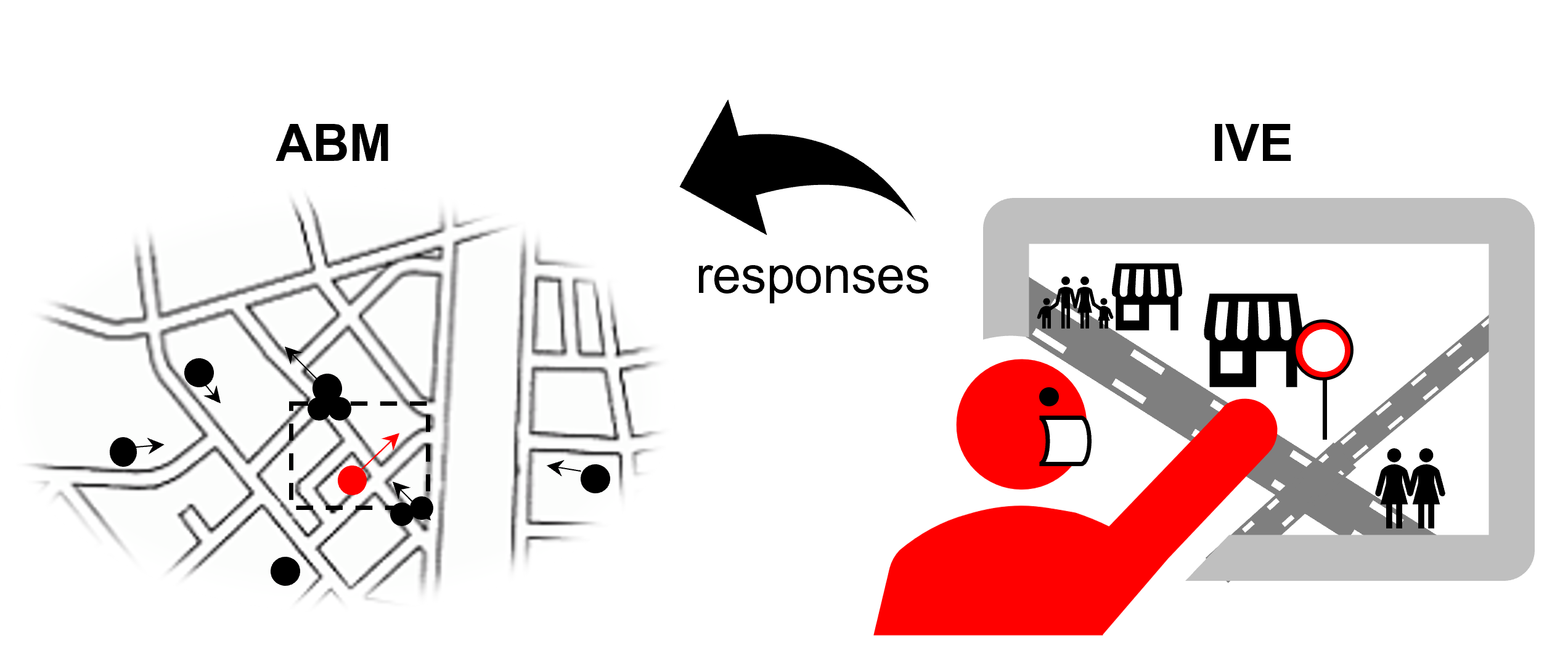
In order to overcome some of these issues, we propose a data collection and model calibration method using an immersive video environment (IVE) (Figure 1). An IVE realistically simulates real-life streetscapes in the lab through video footage that can be enhanced with overlays (Du et al. 2020). Although an IVE can be classified as a type of virtual reality (VR), it offers distinct advantages over traditional VR methods that rely on computer-generated simulations and headsets. An IVE does not require a headset, which solves the problems of interference with face masks and hygiene concerns. User experiments can thus be conducted in a safe and reproducible way during a pandemic. Furthermore, the scenes in the IVE are created using video footage instead of computer-generated simulations, which reduces the effort required for scene production and enhances the objectivity of the experience. This allows the IVE to visualize streetscapes, including potential interventions, in such a way that the participants can experience them with a high degree of realism (Snowdon & Kray 2009). Previous work has indicated that virtual experiments can be a valid method of studying pedestrian behavior, as demonstrated by strong correlations between navigation behavior in virtual environments (e.g., an IVE) and the real world (Coutrot et al. 2019; Delikostidis et al. 2015; Li et al. 2019).
The method is demonstrated by setting up an agent-based model of pedestrians responding to the effects of potential COVID-related streetscape interventions. The specific policy intervention we evaluate is to place one-way street signs for pedestrians to facilitate and stimulate physical distancing. While our previous work reports on data collected in the user study (Stenkamp et al. 2023), the current paper is about how behavioral responses to these interventions, including uncertainty, are derived from the collected data by means of regression bootstrapping, and how these are then combined with rules of pedestrian behavior to form an ABM. With the ABM, we aim to answer the following research questions: 1) How are pedestrian densities influenced by one-way street signs? and 2) How does this influence vary with the number of people and number of street signs?
Methods
The city center of Quakenbrück (Lower Saxony, Germany) was used as study area. We first conducted a user study in the IVE to derive behavioral responses of the participants to one-way street signs for pedestrians. Then, the ABM was set up. Next, we performed a calibration, including uncertainty, again with data from the IVE, and performed a sensitivity analysis. Finally, we ran experiments with the ABM to address our two research questions. The following subsections describe the data collection, ABM, calibration, sensitivity analysis, and experimental setup.
Collecting data in the IVE
We carried out a user study in the IVE with 26 participants in February 2022 (Stenkamp et al. 2023), i.e., during an active phase of the COVID-19 pandemic. Therefore, we implemented several precautions. The participant was offered a face mask, hand sanitizer, and a test at a nearby COVID testing centre, all free of charge. The experimenter was tested for COVID daily during the study. During the entire study, the participant and the experimenter wore masks.
At the beginning of the study, participants were instructed to walk to a certain shop to buy something, without any time constraints to reach the destination. In order to isolate the behavior corresponding to the policy measures of interest, we exposed the participants to three different scenarios (Table 1) when navigating. The following instructions were given (one at a time):
- "There is no pandemic (no COVID-19). Pandemic clues such as masks are to be ignored, as the videos were recorded at pandemic times."
- "There is a pandemic, with infection incidence similar to the current one. The municipality implements the measures currently in force."
- "There is a pandemic, with infection incidence similar to the current one. The municipality has introduced additional measures for pedestrians."
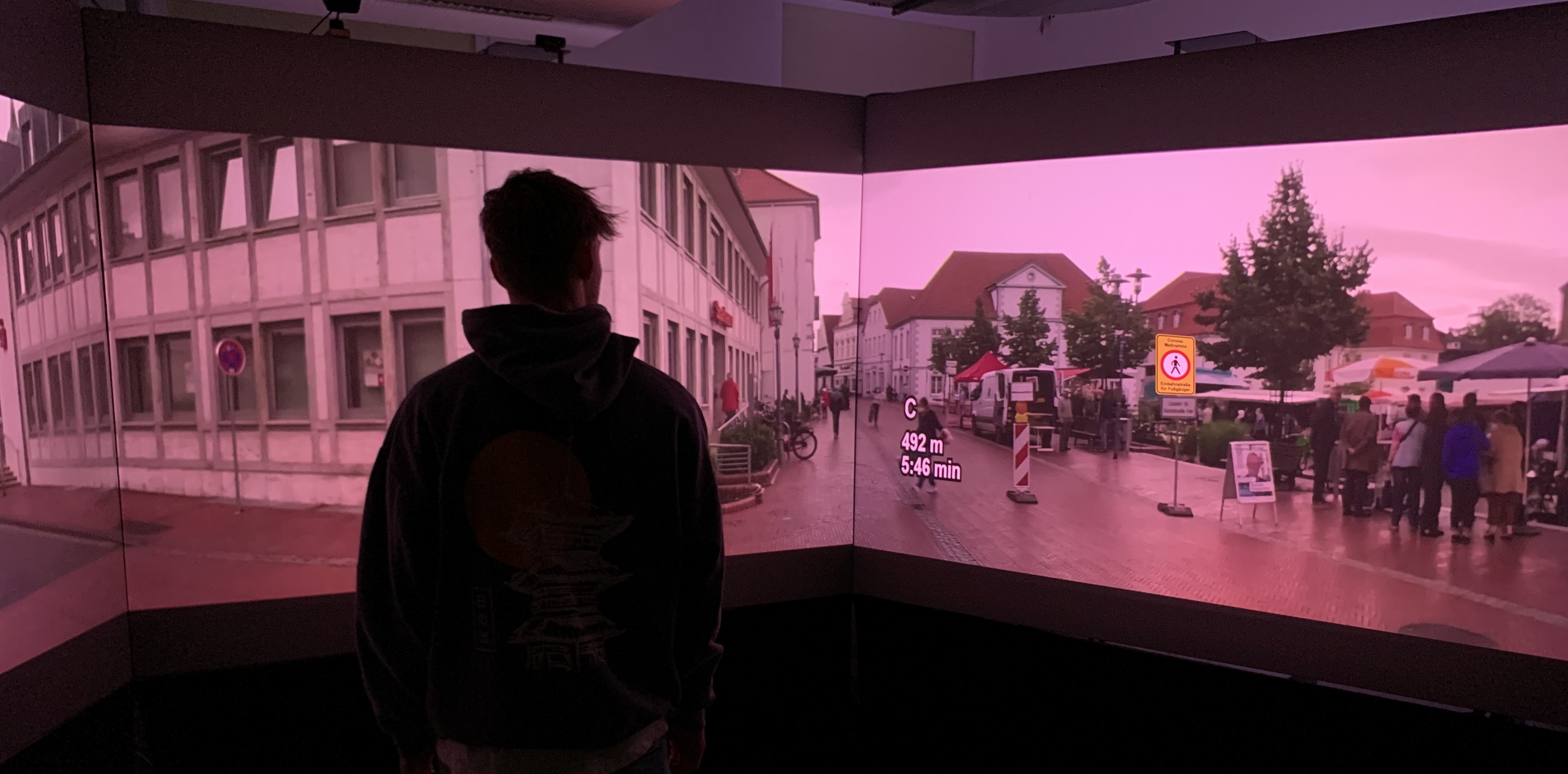
In the IVE, real-world footage of street intersections was shown and overlayed with contextual information (Figure 2). In all scenarios, we displayed overlays indicating the metrical and temporal distance from the current decision point to the destination for each available routing option (see Figure 2, info for option C). In the third scenario, we had additional overlays representing the implemented policy measures: street signs indicating one-way streets for pedestrians, one for the allowed direction and one for the forbidden direction (see sign on the right-most screen in Figure 2, Table 1).
At the decision points, participants had to verbally announce where they wanted to go. After one of the options was selected, a transition to the next decision point on the route was shown. It consisted of a slide show depicting the walk from the current to the next decision point along the chosen path. Throughout the study, the participants navigated three different routes, one per scenario, under a Latin square design to prevent order effects. After completing all three routes, participants were asked to fill in a questionnaire (with questions about, among other things, which factors had affected their decisions), and received a compensation of 15 euro for their time. For a more detailed description of the user study, see Stenkamp et al. (2023).
The data were logged at each decision point by participant and by scenario. During post-processing, these data were matched to the possible options at the corresponding decision points, including the distance to the destination for each option. This resulted in a set of variables for deriving behavioral rules and model calibration (cf. Appendix B, Tables 6 and 7).
Behavioral responses to interventions
To evaluate if the presence of the pandemic (scenario 2 and 3) and/or the placement of the street signs as a policy measure (scenario 3) had an effect on the behavioral responses of our participants, we performed a Welch’s analysis of variance on the three scenarios followed by pairwise Games–Howell post-hoc tests. We did this for two variables: the normalised observed detour and the trespassing count (Table 1 and Table 2). For both variables, a significant difference in the mean was found between scenarios 1-3, and 2-3, but not between scenarios 1-2 (Table 2) (Stenkamp et al. 2023). This implies that the pandemic alone did not significantly change the route choice of the participants, while the presence of the street signs did. The mean detour went up in presence of the signs, while the trespassing count went down (Table 1). This is in line with the statements of our participants in the questionnaire that they were influenced by the street signs in their decisions, and that they were willing to avoid closed (one-way) streets and take a detour in order to comply with the policy measures.
| Scenario | Pandemic | Signs | Mean values | |
| NOD | TC | |||
| 1 | ✘ | ✘ | 10% | 2.13 |
| 2 | ✓ | ✘ | 22% | 2.10 |
| 3 | ✓ | ✓ | 47% | 1.23 |
| Scenarios | Pairwise Games-Howell tests | |
| NOD | TC | |
| 1 - 2 | \(\textit{p} = .125\) | \(\textit{p} = .975\) |
| 1 - 3 | \(\textit{p} < .001\) ** | \(\textit{p} < .002\) ** |
| 2 - 3 | \(\textit{p} = .015\) * | \(\textit{p} = .002\) ** |
| * significance at a confidence level of 95% | ||
| ** significance at a confidence level of 99% | ||
Yet, the fact that the trespassing count did not fall to zero in scenario 3 (Table 1), means that not all participants consistently complied with the installed measures. This is in line with the result of a question in the questionnaire where we asked for an acceptable length of detour. Only two participants would accept a detour of any length, while the accepted detour for the others was on average 363 m for a 1000 m route. Spearman’s correlation between this stated detour and the observed detour in scenario 3 was found to be strong (0.75) and significant.
As such, we concluded that we require a rule in our ABM that make agents observe the one-way street signs, and evaluate whether or not to comply with it. This evaluation is influenced by (at least) the length of the expected detour. The next subsection explains the ABM, including this rule, in detail, while the subsequent subsection outlines how we calibrated the ABM with the data from the user study.
Model
In the following sections, the agent based model is described using the ODD protocol (Grimm et al. 2006, 2010, 2020). The model’s source code and related data are publicly available at https://doi.org/10.5281/zenodo.10471242 (Karic et al. 2024).
Purpose
The main model purpose is to evaluate the change in pedestrian movement flows due to the implementation of streetscape interventions during a pandemic such as the COVID-19 pandemic. The intervention we focus on in this paper is the installation of one-way streets for pedestrians. The central idea of the model is that pedestrians do not always comply with interventions, i.e., they violate the rules in certain situations (see Section 2.7 ff.). The model aims at modelling the agent’s decision whether or not to comply with interventions at street intersections and the resulting city-wide movement patterns and crowdedness of streets.
Entities, state variables, and scales
Agents: Agents in the model represent pedestrians. They possess six static attributes, which vary between agents but are fixed during the simulation. These are their identity number, their walking speed in \(m \cdot s^{-1}\), a destination and weighting factors for importance of (1) length of a detour, (2) presence of a one-way street and (3) general likeliness to reroute (Table 3, type static). The three weighting factors are part of an agent’s rerouting behavior and were calibrated within this work (cf. Section 2.28). Pedestrians also have dynamic attributes that vary between agents as well as over time steps (i.e., agent states). Pedestrians’ dynamic attributes are their position on a street network, an intended route towards the destination, and the detour taken so far (Table 3, type dynamic).
| Attribute | Type |
|---|---|
| identity number | static |
| walking speed in \(m \cdot s^{-1}\) | static |
| destination | static |
| weighting factor for length of a detour | static |
| weighting factor for presence of a one-way street | static |
| weighting factor for general likeliness to reroute | static |
| current position on a street network | dynamic |
| intended route towards the destination | dynamic |
| detour taken in \(m\) | dynamic |
Spatial units: There are two types of spatial units used in the model, street segments and intersections. Street segments are characterised by an identity number, their starting and ending positions and a list of coordinates in between these in a metric coordinate system, their width in meters, the intersections they are connected to, and the intervention placed on the street segment. Intersections are characterised by an identity number, a position and the streets they are connected to.
Environment: The environment is a city, characterised by the layout of the street network, the pandemic situation (pandemic or no pandemic), the total number of agents present in it, and the presence of streetscape interventions (number and location of one-way streets).
Temporal and spatial resolutions: One time step in the model represents 5 seconds in reality. This time step size is chosen based on pedestrian speeds and the length of the shortest street segment, to ensure that agents do not skip a street segment between time steps. The temporal extent is 60 minutes. The street network is represented as a graph in the metric coordinate reference system EPSG:5652.
Process overview and scheduling
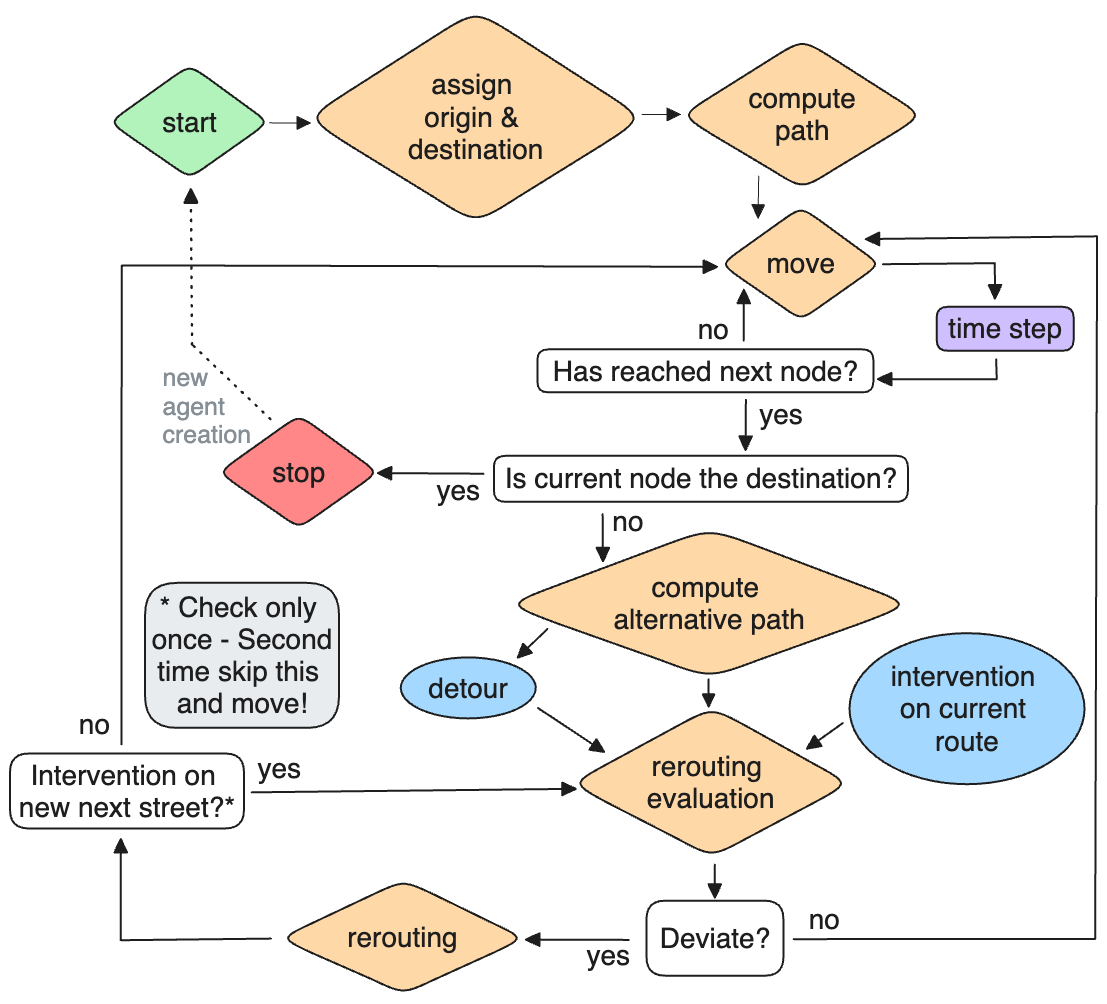
Before the first time step agents are initialized (see section Initialization). During subsequent time steps, agents positioned on a street segment walk for the duration of a time step (the distance they cover depends on their speed) or until they reach the next intersection (Figure 3). Each agent positioned on an intersection checks what alternative route (next shortest route) there is besides its intended route. Based on interventions on the next street segment of their current route and on the length of the detour imposed by the alternative route, the agent takes a decision (keep intended route or reroute). The decision process is described in the rerouting evaluation sub-model (cf. Section 2.27). If the agent decides to keep the intended route, it walks for the duration of a time step along the next street segment. The same happens if the agent decides to reroute and there is no intervention present on the first street segment. In case there is an intervention on its new intended route, it may decide to reroute again, but only once. When an agent reaches its destination, it stops. It then gets a new origin and destination assigned and follows the same procedure as a newly initialized agent.
Design concepts
Basic Principles. This model extends earlier models of pedestrian movement behavior within cities, where route choice is based on the shortest path or least angular change (Omer & Kaplan 2017). In our model, agents also compute the shortest path, but can deviate from it, either spontaneously or influenced by physical-distancing measures implemented in the streetscape in the light of an ongoing pandemic.
Adaptation. Initially, each pedestrian computes the shortest path to its destination. If they are at an intersection, they may adapt their path based on a rerouting evaluation process.
Learning. Agents in our model do not learn.
Sensing. We assume that the agents are familiar with the city, but that the interventions are new to them. Consequently, agents have complete information about street lengths and connection of streets in the street network, but they can only see streetscape interventions for streets that are connected to an intersection they are located at.
Stochasticity. There are four stochastic processes in the model: (1) origin and destination of each agent is set randomly, with the condition that they are a minimum of 250 m. apart, (2) the walking speed of agents is drawn from a Gaussian distribution with a mean of 1.25 \(m \cdot s^{-1}\) and a standard deviation of 0.21 \(m \cdot s^{-1}\) (Chandra & Bharti 2013), (3) intercept and weighting factors for the agents’ rerouting evaluation function are drawn from Gaussian distributions, for which the mean and standard deviation are calibrated (see Calibration section), and (4) the decision-making process to reroute at an intersection, which is based on the probability resulting from the rerouting evaluation function.
Observation. The variables we collect from the model are (1) agent positions for each time step, (2) pedestrian density at each street segment for each time step, (3) number of passers-by, reroutings, compliances and non-compliances at each intersection at each time step, (4) the normalised detour of each route of an agent and (5) the non-compliance probability at intersections with one-way streets.
Initialization
At the initialization, intersections, streets, and interventions are loaded from a geopackage file into the model. Streets and intersections are translated into a graph in which intersections become nodes and streets segments become edges. The weight of an edge is the metric length of the corresponding street segment.
Furthermore, a model run is initialized with the given number of agents (\(N\)), number of time steps (\(T\)), duration of a time step in seconds (\(d\)), a distribution of agent walking speeds in \(m \cdot s^{-1}\) (\(ws\)), a scenario (\(S\)) that describes the number and location of streetscape interventions, distributions of intercept (\(\alpha\)) and weights (\(\beta_{rtd}\), \(\beta_{forbidden}\)) for the rerouting evaluation function (cf. Calibration section) (Table 4).
Agents are initialized with their specific intercept (\(\alpha_j\)) and weighting factors (\(\beta_{j,rtd}\), \(\beta_{j,forbidden}\)) for the rerouting evaluation function, a fixed walking speed (\(ws_{j}\)), an origin, and a destination (Figure 3). Agents are positioned at their origin. They compute the shortest path between their position and the destination.
| Parameter | Description |
|---|---|
| \(N\) | Number of agents |
| \(T\) | Number of time steps |
| \(d\) | Duration of one time step |
| \(S\) | Scenario |
| \(ws\) | Gaussian distribution of walking speeds |
| \(\alpha\) | Gaussian distribution of regression intercept in rerouting evaluation |
| \(\beta_{rtd}\) | Gaussian distribution of regression weights for relative total detour in rerouting evaluation |
| \(\beta_{forbidden}\) | Gaussian distribution of regression weights for a one-way street sign in rerouting evaluation |
Input data
The model uses a street network from the city of Quakenbrück, Lower Saxony, Germany as input data. The data is extracted from OpenStreetMap (OSM). For the street width estimation we used the existing OSM classes residential (street with two sidewalks and vehicle traffic), path (narrow trail, no vehicle traffic) and living street (broad street designed for pedestrians, allowance of slow vehicle traffic). Streets that were missing a label were classified via aerial images using the ‘GeobasisdatenViewer Niedersachsen’ (Landesamt für Geoinformation und Landesvermessung Niedersachsen (LGLN) 2023). To estimate the street widths 10 sample-measurements of the walkable area were taken per class using the ‘draw/measure’ tool offered by ‘GeobasisdatenViewer Niedersachsen’. The resulting walkable width of a residential street was 5 meters, a path was 3 meters, and a living street was 10 meters.
Submodels
The only submodel is the rerouting evaluation function that each agent has. It is run for each agent j that is standing at an intersection and evaluates whether to stay on the intended path. The probability to stay on the intended (usually the shortest) path is influenced by the presence of interventions as well as the relative length of the total detour \(RTD_j\) the agent expects to take. \(RTD_j\) is composed of three factors:
| \[ RTD_j = \frac{D_j}{(TPL_j + RSPL_j)}\] | \[(1)\] |
These three factors are: 1) The length of the detour \(D_j\) that agent j would need to take when rerouting, defined as the difference between the lengths of the intended path, \(p_{j,i}\), and the alternative path, \(p_{j,a}\), as:
| \[ D_j = length(p_{j,a}) - length(p_{j,i})\] | \[(2)\] |
| \[ RSPL_j = length(p_{j,s})\] | \[(3)\] |
| \[ TPL_j = length(p_{j,t})\] | \[(4)\] |
Then the probability to stay on the current route, \(P_{j,stay}\), is defined as logistic function in terms of \(RTD_j\) as:
| \[ P_{j,i,a,stay} = \frac{1}{1 + e^{- (\alpha_{j} + \beta_{j,rtd} * RTD_j + \beta_{j,forbidden} * FORBIDDEN_i)}}\] | \[(5)\] |
Calibration
To calibrate the weights in the rerouting evaluation function, binary logistic regression was applied to the participant data collected in the IVE. Multiple independent variables (cf. Appendix B) that we considered potentially relevant were included, using a leave-one-out procedure in the calibration until only statistically significant variables were left. The significance of a variable for the regression model was measured by the p-value. As a threshold for a variable to be statistically significant 0.05 was set.
The final logistic regression model had only two significant independent variables, \(RTD\) and \(FORBIDDEN\), and thus had the form:
| \[ z = \alpha + \beta_{rtd} * RTD + \beta_{forbidden} * FORBIDDEN\] | \[(6)\] |
| \[ \theta = pr(Y = 1) = \frac{e^{z}}{1+e^{z}}\] | \[(7)\] |
In this case, the event to model was whether a participant takes the shortest path. \(\beta_{rtd}\) and \(\beta_{forbidden}\) are the coefficients of the explanatory variables \(RTD\) and \(FORBIDDEN\), and \(\alpha\) is the intercept. The coefficients are estimated using maximum likelihood (Cox 1958). Preparing the data for the regression, categorical variables are converted to indicator variables. The data are split in training and test data to allow an independent check of the quality of the model.
In order to calibrate the agent decision function, we use a bootstrapped regression. Bootstrapping is random sampling of the data in any test or metric (Fox 2015). A regular (single) regression has two downsides: (a) the fact pedestrians vary in their behavior is not reflected and (b) our data has a sample size of only 26 participants as the IVE study is time-consuming. Bootstrapping solves these two downsides. We use the most straightforward form of bootstrapped regression (Fox 2015), which involves collecting the values of the dependent and two independent variables for each of the \(n\) observations, and then for each bootstrap sample \(b\) = 1,... , \(r\), randomly draw \(n\) observations \(b_{n}\). Consequently, a regression is performed on each bootstrap sample, producing \(r\) sets of bootstrap regression coefficients. Although this method has also been implemented in the JAS-mine platform, designed to calibrate microsimulations in the microeconometrics domain (Richiardi & Richardson 2017), we have not found it been applied to any ABM use case.
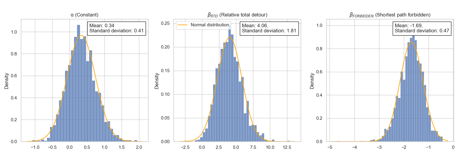
Our training data are resampled with replacement in 2000 bootstrap samples (considered a large enough sample as suggested by Fox 2015), for which a logistic regression model is calculated. As a result, we obtain 2000 results for \(\alpha\), \(\beta_{rtd}\), and \(\beta_{forbidden}\). Together, these form distributions of the corresponding variables, for which we computed a mean and standard deviation. These are used to draw values of \(\alpha_j\), \(\beta_{j,rtd}\), and \(\beta_{j,forbidden}\) such that different agents in the ABM have different intercepts and weights in their rerouting evaluation function.
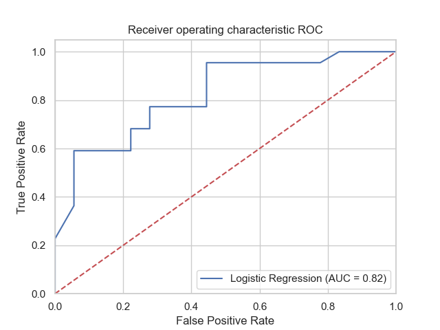
We test the accuracy of the different potential rerouting functions of the agents by picking values from the distribution of intercept and weights, again 2,000 times. As a measure for the quality of the regression function the accuracy score, which is the fraction of correct predictions, is computed on the test data. Additionally, we plot the Receiver Operating Characteristics (ROC) curve, which shows the True Positive Rate against the False Negative Rate - in our case for the correct or incorrect prediction of a pedestrian to stay on the shortest path - at different classification thresholds against each other. Then we compute the Area Under the Curve with its possible value ranking between 0.0 and 1.0. Herein, 0.0 means at every threshold all the predictions are wrong and 1.0 means all predictions are correct. A model that performs equal to a random classification is represented by a diagonal curve, with an AUC value of 0.5.
We use the Python package statsmodels (Seabold & Perktold 2010) for the binary logistic regression and scikit-learn (Pedregosa et al. 2011) for its testing.
Sensitivity analysis
As the parameters in the model are expected to interact, a local sensitivity analysis may not give valid results (Saltelli & Annoni 2010), so we opt for a global sensitivity analysis, also referred to as variance contribution method. We performed a Sobol’ Sensitivity Analysis (Sobol 2001), which assesses the contribution of each parameter’s uncertainty to the total variance in the model outputs, whilst also considering interactions (Convertino et al. 2014). With this method, we test the sensitivity of (1) the non-compliance probability and (2) the normalised detour (cf. Section 2.22) to the uncertainty in four model parameters: \(\alpha\), \(\beta_{rtd}\), \(\beta_{forbidden}\), and \(ws\). The uncertainty in the parameters is quantified by the bootstrapping (cf. Section 2.25) for \(\alpha\), \(\beta_{rtd}\), and \(\beta_{forbidden}\), and from literature for \(ws\) (Chandra & Bharti 2013).
The sensitivity analysis was conducted using the SALib Python package (Herman & Usher 2017) with Saltelli sampling (Saltelli 2002). To find a suitable sample size, it was increased repeatedly until the Sobol’ index values converged (Nossent et al. 2011). As a result the number of samples was 1024 and the number of model runs was 10240.
Experimental design
One default model run and two experiments are run, corresponding to our two research questions (Table 5). The first experiment assesses the effect of one-way street signs on pedestrian densities by comparing the output of a run with eight interventions with the output of a run with the same number of pedestrian agents but without interventions. Furthermore, we compare the output of the model with a calibrated rerouting function with a version of the models in which all agents always comply with all interventions. This provides information on the necessity of our data collection effort on compliance in the IVE.
| Experiment | Agents | Interventions | Compliance behavior | Total runs |
|---|---|---|---|---|
| default | 4000 | 8 | calibrated | \(1\) |
| RQ 1 | 4000 | 0, 8 | calibrated and full | \(2*2-1^*=3\) |
| RQ 2 | 2000, 4000, 8000 | 0, 4, 8, 10 | calibrated | \(3 * 4 = 12\) |
The second experiment assesses how variations in number of pedestrians and number of interventions influence the effect that was found in the first experiment. Hereto, in relation to the default run, we perform runs with fewer (2000) and more (10000) agents, as well as fewer (4) and more (10) interventions. A zero-intervention benchmark is added again, resulting in 12 runs. To account for the effects of stochasticity, all model runs are performed 10 times. Besides comparing among the different runs, we compare modelled pedestrian densities with a threshold of \(0.16 \, people / m^2\) at which people can no longer maintain a 1-m. distance at all times (Echeverrı́a-Huarte et al. 2021).
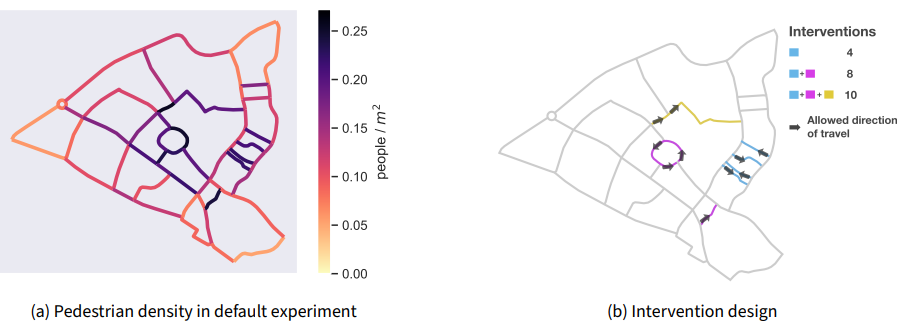
In order to decide where to place the interventions, we use the results of the default run (Figure 4a). Interventions are placed at street segments with the highest pedestrian densities. The direction of the one-way street is chosen opposite for parallel one-way streets if present, and in the same direction for connected one-way streets (resulting in one "roundabout"), and otherwise randomly, see the resulting intervention design in Figure 4b.
Results and Discussion
Calibration
The 2000 bootstrap samples led to Gaussian-shaped distributions of the intercept and weights in the rerouting evaluation function (Figure 5). The relative total detour the pedestrian traversed so far (until the current intersection) has a positive relation with staying on the intended path. In other words, when the pedestrian already has already taken long detours (either by free choice or pressed by the interventions), it becomes less willing to take detours again. Interventions on the intended path have a negative relation with staying on the path. That means that interventions stimulate the pedestrian to decide to reroute.
The regression functions using intercepts and weights from these distributions had an accuracy with a mean of 0.66 and an AUC of 0.82 (see ROC curve in Appendix A). This suggests that they capture relatively well when a pedestrian decides to reroute and that they do so substantially better than a random model.
Sensitivity analysis
The variance in the mean non-compliance probability is mainly determined by the weight of the interventions \(\beta_{forbidden}\) (47%) and by the regression constant \(\alpha\) (45%), while the variance in the mean normalised detour is mainly determined by the weight of the relative total detour \(\beta_{rtd}\) (47%) and also by the regression constant \(\alpha\) (32%) (Figure 6). This implies that, as expected, the uncertainty in the compliance component in the regression function has the largest impact on overall compliance uncertainty in the ABM output. In contrast, the uncertainty in the compliance component in the regression function has a low influence (2%) on the mean modelled detour of the pedestrians. This is due to the distribution of \(\beta_{forbidden}\) being narrow (Figure 5), pedestrians taking detours irrespective of interventions, and to the fact that many of the routes chosen by pedestrians do not contain interventions. In the context of setting up the ABM this is a benefit as it means that setting this hard-to-determine weight is not crucial for the detour pedestrians take.
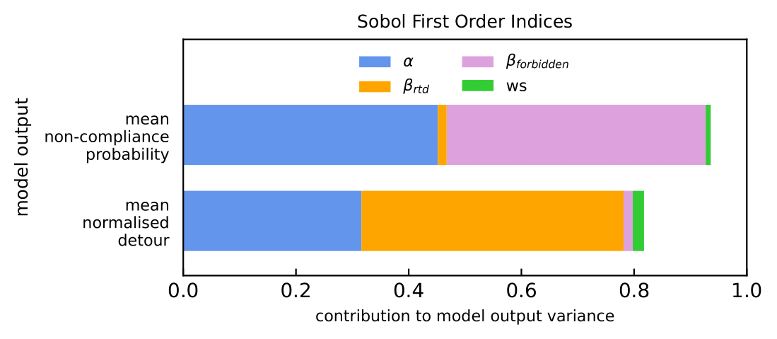
In total, the first-order effects of the parameters explain 82% of the variance in the mean normalised detour and 93% of the variance in the mean non-compliance-probability. The remaining variance is caused by second or higher order effects, i.e., by interactions between the parameters (Convertino et al. 2014). Given that the higher-order effects are relatively small, we did not look further into them.
Effect of one-way street signs on pedestrian densities
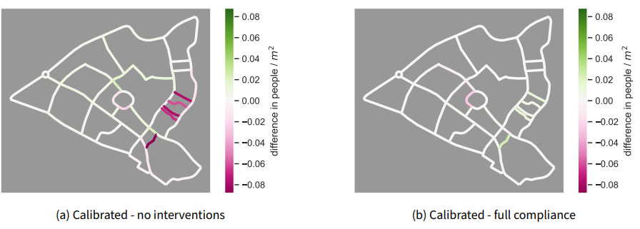
The results of the first experiment (RQ1, Table 5) show a reduction in the average pedestrian density on all streets with interventions. Five out of eight one-way streets have a large reduction of \(0.060\) to \(0.088 \, people / m^2\) (Figure 7a). For the other three one-way streets, which were installed to form a pedestrian roundabout (Figure 4b), the reductions were smaller, \(0.0030\) to \(0.023 \, people / m^2\). This was probably due to the pedestrians not having to take a big detour when simply following the roundabout in the "correct" direction. All streets without interventions have differences in the range of \(-0.017\) to \(+0.022 \, people / m^2\). Since pedestrian density was reduced in the targeted streets, but not largely increased in any other street, pedestrian one-way streets may be a useful tool to reduce crowding and stimulate physical distancing in cities during pandemics.
Comparing our calibrated model with a version of the model in which all agents always comply with all interventions (still RQ1, Table 5), resulted in little change in average pedestrian densities (Figure 7b). For streets without interventions the largest difference is a decrease by \(0.0090 \, people / m^2\) in the full compliance model version. Also differences on one-way streets were small, ranging from \(-0.027\) to \(+0.024 \, people / m^2\). Half of these streets differed by less than \(0.010 \, people / m^2\). The limited magnitude of these differences suggests that calibration of pedestrian behavior may not be necessary when simulating pedestrian density. Consequently, assuming full compliance might suffice to observe relevant changes in pedestrian density – at least for the street layout, interventions and crowd sizes we used in our study.
Effect of variations in pedestrians and interventions
The second experiment (RQ2, Table 5) shows that, independently of the number of interventions, streets become more crowded as the number of agents increases (Figure 8). At a low number of agents (2000 agents; Figure 8, left) the interventions have little effect on the pedestrian densities.
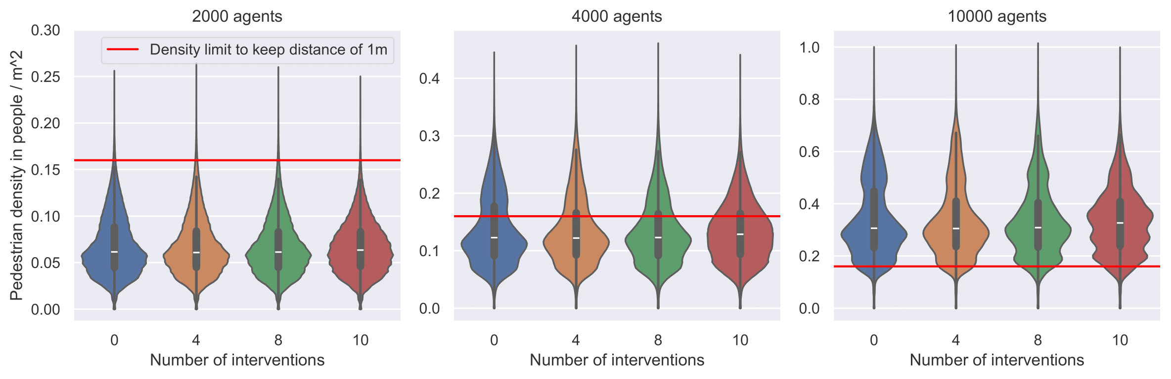
For a medium number of agents (4000 agents; Figure 8, center), the third quartile of densities in the no-intervention run lays above the critical threshold. Adding interventions shifts the third quartile closer to the threshold. With more interventions, we observe a stronger downward trend at high densities, especially above \(0.2 \, people / m^2\). Thus, for a medium number of agents, interventions reduce pedestrian densities on streets with critical densities. At the same time, the overall compliance rate goes down from 83% (4 interventions) to 79% (8 interventions) to 72% (10 interventions), making the density reduction lower than it could have been. The reduction in compliance rate is caused by the influence of the detour: more interventions cause a longer detour, which makes the agents less willing to comply when they encounter another intervention.
At a high number of agents (10000 agents; Figure 8, right), even the first quartile is above the critical threshold in the no-intervention scenario, i.e., there is a high number of streets with critical pedestrian densities. Adding four or eight interventions helps to lower the third quartile, thus very high numbers of densities, though not to below the critical threshold of \(0.16 \, people / m^2\). Interestingly, with this high number of agents, increasing the number of interventions to ten, increases the number of streets with critical pedestrian densities, i.e., the opposite of what the interventions are to achieve. Such an effect can indeed occur in reality because of the increased length of pedestrians’ routes; when they have to walk more, more pedestrians are on the streets, and the streets are more crowded. This effect is more prevalent in the increase from eight to ten interventions, than in the increase from four to eight because of their placement: the increase from four to eight in mainly the installment of the pedestrian roundabout (Figure 4b), which does not increase the length of the agents’ routes much, since they only need to travel this roundabout in the correct direction, as noted earlier. The authors acknowledge that caution is advised when interpreting the model outputs with a high number of agents, since they did not test or calibrate for possible effects of large crowds on individual agents’ decisions. Further testing on the effects of crowding on compliance behavior is necessary to ensure validity in these cases, on which we elaborate in Section 3.17.
Overall, we conclude from this second experiment that the introduction of one-way streets is beneficial or neutral in most cases. In addition to the neutral to positive effects described above, one-way streets allow higher walking speeds than two-way streets at the same density and cause fewer crossings of people, i.e., lower chances of short distances between pedestrians at the same density (Teknomo 2006). However, since we currently use densities as a measure instead of distances between pedestrians, our model is not able to show these additional positive effects.
Results in the context of existing work
Other studies on the effects of streetscape interventions during the COVID-19 pandemic confirm the willingness of participants to comply with one-way streets found in our work (McCormack et al. 2022). The compliance-percentage with one-way streets in the default scenario (79%) is similar to reported compliance with physical-distance measures in general by Beca-Martı́nez et al. (2022) of 85%. Also, the effect of pedestrian one-way streets on reducing crowd densities is in line with other work (Blibli & Bouchair 2023).
The respondents of a survey of Briscese et al. (2020) indicated that duration of exposure to interventions (in this case self-isolation) would not have an effect on their compliance. The results of our regression contradict this finding: the longer the cumulative detour, the less likely pedestrians became to comply with additional interventions. This difference supports our appeal for an experimental design that can test actual responses as opposed to stated preferences; people may overestimate their patience or perseverance when being asked in a survey.
Yet, another effect observed by Briscese et al. (2020) could be said to match with our results: when respondents were negatively surprised by a given hypothetical extension of a measure, i.e., if the extension was longer than what they expected, they stated to be less likely to comply. Given that our pedestrians did not know in advance where and how many one-way streets would occur during their walk, the decrease in likeliness to comply with increasing detour could be due to being surprised to find more interventions than expected towards the end of their route.
Limitations and future work
Although we were able to derive conclusions about the effects of streetscape interventions on pedestrian densities and the variation in this effect under different conditions, our work is subject to a number of limitations. Firstly, when looking at the effects of interventions, we varied the number of pedestrians present in the city and the number of interventions. Yet, we did not vary the locations of these interventions. We placed the interventions at locations that had the highest pedestrian densities in the default (benchmark) scenario, but this does not necessarily mean that these locations are optimal to distribute the pedestrians over the city. An optimization of intervention locations (e.g., Zhang et al. 2020) was beyond the scope of this study and could be an interesting topic for future work. Furthermore, dynamic instead of static signs could be tested as interventions (Langner & Kray 2014), as these can be adapted to pedestrian densities in real time.
Secondly, we applied the model to a single case study area. Our case study area is in Germany, and the city has a typical European layout with a central square and irregular street pattern; the detours pedestrians have to take upon road closure compared to American grid-shaped cities are therefore often longer. The number of participants in our case study was limited to 26 and all of these participants were German. Thus, our results, especially the compliance rates, are tied to the German context in terms of cultural dimensions (Hofstede 2011; Kruelen et al. 2022), such as individualism versus collectivism (the need for autonomy (Kruelen et al. 2022) or self-interest to efficiently reach the destination versus disease risk for others) and short-term versus long-term orientation (saving some minutes by not complying with a one-way street or risking getting ill in a few days). Consequently, we do not claim generalizability of our results beyond this case study. In contrast, we aimed to present a general and reproducible procedure with an ABM connected to an IVE to collect data for deriving agent behavior and for calibration, making it easy to set up a model for any case study at hand.
Thirdly, the base route-choice behavior of our agents, before adding the pandemic-specific factors, was simplistic. We assumed that agents have complete information about the layout of streets and applied a shortest-path algorithm to compute the initial path of the agent from origin to destination, while recent research has stressed that pedestrians route using their mental map that is imprecise and contains elements such as landmarks (Filomena & Verstegen 2021) and regions (Filomena et al. 2020). We believe it is justified to use a simplistic base behavior here for two reasons: 1) the studied city is small and consequently there are limited route-choice options and they are easy to remember for the pedestrians, and 2) our main aim in this paper was to demonstrate the set up of an ABM with data from the IVE, which is easier to illustrate with a relatively simple base behavior.
Finally, while we investigated the potential effects of several factors on pedestrians’ behavior in our logistic regression with data from the IVE (and found only two relevant factors), an important factor was not considered: crowdedness of streets. It is expected that the likelihood to comply with one-way streets increases with the crowdedness of these streets because crowded places are seen as a high risk of infection (Beca-Martı́nez et al. 2022). This may increase people’s awareness of the need for an intervention to stimulate distance-keeping for their own safety as well as for the safety of others. In addition, in crowded situations people are expected to act according to the principle of social proof (Cialdini 1993; Cialdini et al. 1999; Goethals & Darley 1977). Thus, individuals may adjust their willingness to comply with interventions based on the compliance behavior of others. One potential effect is that other people who comply may be perceived as supervisors/controllers prompting compliance (Brehm & Gates 1993). Simultaneously, the transgression of others may reduce individuals’ willingness to comply with interventions. We were not able to include this effect in our model, because the previous user study that provides us with the data to calibrate the model (Stenkamp et al. 2023) did not systematically vary crowdedness. Crowds being a dynamic feature makes overlaying them on the videos in the IVE more challenging; this is a line of future work (Schröder et al. 2023).
A related opportunity for future work is a closer link between ABM and IVE. Currently, this is a one-way coupling: experiments from the IVE feed into the ABM through the design of our rule set and calibration. Re-evaluating situations with high uncertainty in the ABM within the IVE could create a promising feedback loop. As an example, an agent reaching an intersection with a 50% probability to reroute, could be transferred to a scene in the IVE with the corresponding intersection characteristics to be presented to a number of study participants. Such setup requires the ability to dynamically generate scenes based on provided intersection parameters, for which proof-of-concept has been attained recently (Schröder et al. 2023).
Conclusion
In this work, we presented a method to set up and calibrate an ABM using an immersive video environment (IVE). We derived behavioral rules and built an agent-based model of pedestrians responding to COVID-related policy interventions: street signage for pedestrians. We identified the need for a behavioral rule that can evaluate whether to deviate from an intended path, taking into account observed street signs and the distance to a pedestrian’s intended destination. Using regression and bootstrapping, we calibrated the model while preserving heterogeneity in behavior between different pedestrians.
We investigated the effects of streetscape interventions during the COVID-19 pandemic on pedestrians movement. With the designed agent-based model we addressed the following research questions: 1) How are pedestrian densities influenced by one-way street signs? and 2) How does this influence vary with the number of people and number of street signs? The city center of Quakenbrück (Lower Saxony, Germany) was used as study area. To answer the first research question, we ran the model with and without one-way street signs. Comparing the average difference in pedestrian densities across all streets, we found a decrease in pedestrian densities on all streets with interventions. Meanwhile, there was no significant increase in any street. That is, the street signs had their intended effect.
For our second research question, we varied the number of pedestrians in the model and the number of one-way streets in the street network. We found that the interventions are effective in reducing pedestrian densities below the critical threshold up to a medium number of pedestrians. When the number of pedestrians in the area is very high, adding more interventions can also increase pedestrian densities, i.e. have the opposite effect of what was intended.
The main contribution of our work is two-fold. The first is the data collection and calibration method for agent-based models in the IVE that provides a basis for future testing of other existing or potential policy interventions. The data collection method allows user studies to be carried out safely without exposing participants to potentially hazardous situations in the real world during a pandemic. Furthermore, the situation that the participant is exposed to is fully reproducible, and thus comparable between participants. This is nearly impossible in real-world studies, where factors like weather conditions and traffic vary naturally. The bootstrapping regression as a calibration method for agent-based models is useful for model cases with small samples and uncertainty. Our second contribution entails the understanding of pedestrian movement dynamics during pandemics such as the COVID-19 pandemic, in particular the behavioral responses to potential interventions in the physical environment. The model we proposed in this work contributes to ex-ante evaluation of the effects of pedestrian street signage. Our model is available and free and open-source software (Karic et al. 2024) and may be useful in the future given that global epidemics are expected to strike more often due to our increasingly connected world (Briscese et al. 2020).
Appendix A: Receiver Operating Characteristics Curve
Appendix B: Variables (Computed) from the IVE User Study for Deriving Behavioral Rules and Model Calibration
| Variable | Description | Type |
|---|---|---|
| shortest_path | dependent variable for the logistic regression (cf. Calibration Section): IF decision equals shortest path to destination: | boolean |
| shortest_sign | The street sign on the shortest path | categorical |
| shortest_alternate_sign | The street sign on the second shortest path | categorical |
| num_detours | Number of times the participant chose another than the shortest path along this route (unitless) | int |
| num_decisions | Number of decision points traversed (unitless) | int |
| len_traversed | Length of path traversed (meters) | int |
| rem_len_shortest | Remaining distance from the decision point to the destination along the shortest path (meters) | int |
| abs_detour | Detour of the currently second shortest path compared to the shortest path (meters) | int |
| rel_current_detour | Relative detour of the currently second shortest path compared to the shortest (unitless) | float |
| \( rel\_current\_detour = \frac{abs\_detour}{rem\_len\_shortest} \) | ||
| rel_total_detour | Relative detour following the second shortest path divided by the sum of the currently shortest possible remaining path length and the length of the path already traversed | loat |
| \( rel\_total\_detour = \frac{abs\_detour}{rem\_len\_shortest + len\_traversed} \) | ||
| abs_previous_detour | Absolute detour already taken (meters) | int |
| rel_previous_detour | Detour already taken divided by the sum of the currently shortest possible remaining path length and the length of the path already traversed | float |
| \( rel\_previous\_detour = \frac{abs\_previous\_detour}{rem\_len\_shortest + len\_traversed} \) | ||
| Variable | Description | Type |
|---|---|---|
| shortest_path_length | The length of the shortest available path between origin and destination (in meters) | float |
| actual_path_length | The length of the path taken by an participant (in meters) | float |
| norm_obs_detour | Normalised observed detour; Ratio of total detour taken by a participant to the shortest path form origin to destination (unitless) | float |
| \( \text{norm_obs_detour} = \frac{\text{actual_path_length}}{\text{shortest_path_length}} - 1 \) | ||
| tres_count | Trespassing count; Number of times a participant entered roads with signage that forbade entry (unitless) | int |
References
ALEDORT, J. E., Lurie, N., Wasserman, J., & Bozzette, S. A. (2007). Non-pharmaceutical public health interventions for pandemic influenza: An evaluation of the evidence base. BMC Public Health, 7(1), 208.
BECA-MARTÍNEZ, M. T., Romay-Barja, M., Falcón-Romero, M., Rodrı́guez-Blázquez, C., Benito-Llanes, A., & Forjaz, M. J. (2022). Compliance with the main preventive measures of COVID-19 in Spain: The role of knowledge, attitudes, practices, and risk perception. Transboundary and Emerging Diseases, 69(4), 871–882.
BLIBLI, M., & Bouchair, A. (2023). Contribution of numerical simulation to the study of pedestrian mobility in the context of COVID-19: Case of a university campus in Algeria. Architectural Science Review, 66(4), 271–292.
BREHM, J., & Gates, S. (1993). Donut shops and speed traps: Evaluating models of supervision on police behavior. American Journal of Political Science, 37(2), 555–581.
BRISCESE, G., Lacetera, N., Macis, M., & Tonin, M. (2020). Compliance with COVID-19 social-Distancing measures in Italy: The role of expectations and duration. CESifo Working Paper No. 8182. Available at: https://papers.ssrn.com/sol3/papers.cfm?abstract_id=3567556.
BROWN, D. G., & Robinson, D. T. (2006). Effects of heterogeneity in residential preferences on an agent-based model of urban sprawl. Ecology and Society, 11, 1.
CHANDRA, S., & Bharti, A. K. (2013). Speed distribution curves for pedestrians during walking and crossing. Procedia-Social and Behavioral Sciences, 104, 660–667.
CIALDINI, R. B. (1993). Influence: Science and Practice. New York, NY: HarperCollins.
CIALDINI, R. B., Wosinska, W., Barrett, D. W., Butner, J., & Gornik-Durose, M. (1999). Compliance with a request in two cultures: The differential influence of social proof and commitment/Consistency on collectivists and individualists. Personality and Social Psychology Bulletin, 25(10), 1242–1253.
CONVERTINO, M., Muñoz-Carpena, R., Chu-Agor, M. L., Kiker, G. A., & Linkov, I. (2014). Untangling drivers of species distributions: Global sensitivity and uncertainty analyses of MaxEnt. Environmental Modelling & Software, 51, 296–309.
COUTROT, A., Schmidt, S., COUTROT, L., Pittman, J., Hong, L., Wiener, J. M., Hölscher, C., Dalton, R. C., Hornberger, M., & Spiers, H. J. (2019). Virtual navigation tested on a mobile app is predictive of real-world wayfinding navigation performance. PLoS One, 14(3), e0213272.
COX, D. R. (1958). The regression analysis of binary sequences. Journal of the Royal Statistical Society. Series B (Methodological), 20(2), 215–242.
DELIKOSTIDIS, I., Fritze, H., Fechner, T., & Kray, C. (2015). Bridging the gap between field- and lab-Based user studies for location-Based services. In G. Gartner & H. Huang (Eds.), Progress in Location-Based Services 2014 (pp. 257–271). Cham: Springer International Publishing.
DIGNUM, F., DIGNUM, V., Davidsson, P., Ghorbani, A., van der Hurk, M., Jensen, M., Kammler, C., Lorig, F., Ludescher, L. G., Melchior, A., Mellema, R., Pastrav, C., Vanhee, L., & Verhagen, H. (2020). Analysing the combined health, social and economic impacts of the corona virus pandemic using agent-Based social simulation. Minds and Machines, 30(2), 177–194.
DU, G., Kray, C., & Degbelo, A. (2020). Interactive immersive public displays as facilitators for deeper participation in urban planning. International Journal of Human-Computer Interaction, 36(1), 67–81.
ECHEVERRÍA-HUARTE, I., Garcimartı́n, A., Hidalgo, R., Martı́n-Gómez, C., & Zuriguel, I. (2021). Estimating density limits for walking pedestrians keeping a safe interpersonal distancing. Scientific Reports, 11(1), 1534.
FILOMENA, G., Kirsch, L., Schwering, A., & Verstegen, J. A. (2022). Empirical characterisation of agents’ spatial behaviour in pedestrian movement simulation. Journal of Environmental Psychology, 82, 101807.
FILOMENA, G., Manley, E., & Verstegen, J. A. (2020). Perception of urban subdivisions in pedestrian movement simulation. PLoS One, 15(12), e0244099.
FILOMENA, G., & Verstegen, J. A. (2021). Modelling the effect of landmarks on pedestrian dynamics in urban environments. Computers, Environment and Urban Systems, 86, 101573.
FOX, J. (2015). Bootstrapping regression models. In J. Fox (Ed.), Applied Regression Analysis and Generalized Linear Models (pp. 587–606). Thousand Oaks, CA: Sage Publications.
GRIMM, V., Berger, U., Bastiansen, F., Eliassen, S., Ginot, V., Giske, J., Goss-Custard, J., Grand, T., Heinz, S. K., Huse, G., Huth, A., Jepsen, J. U., JNørgensen, C., Mooij, W. M., Müller, B., Pe’er, G., Piou, C., Railsback, S. F., Robbins, A. M., … DeAngelis, D. L. (2006). A standard protocol for describing individual-based and agent-based models. Ecological Modelling, 198(1), 115–126.
GRIMM, V., Berger, U., DeAngelis, D. L., Polhill, J. G., Giske, J., & Railsback, S. F. (2010). The ODD protocol: A review and first update. Ecological Modelling, 221(23), 2760–2768.
GRIMM, V., Railsback, S. F., Vincenot, C. E., Berger, U., Gallagher, C., DeAngelis, D. L., Edmonds, B., Ge, J., Giske, J., Groeneveld, J., Johnston, A. S. A., Milles, A., Nabe-Nielsen, J., Polhill, J. G., Radchuk, V., Rohwäder, M. S., Stillman, R. A., Thiele, J. C., & Ayllón, D. (2020). The ODD protocol for describing agent-based and other simulation models: A second update to improve clarity, replication, and structural realism. Journal of Artificial Societies and Social Simulation, 23(2), 7.
HERMAN, J., & Usher, W. (2017). SALib: An open-source Python library for sensitivity analysis. Journal of Open Source Software, 2(9), 97.
HOEBEN, E. M., Bernasco, W., Suonperä Liebst, L., Van Baak, C., & Rosenkrantz Lindegaard, M. (2021). Social distancing compliance: A video observational analysis. PLoS One, 16(3), e0248221.
HOFSTEDE, G. (2011). Dimensionalizing cultures: The Hofstede model in context. Online Readings in Psychology and Culture, 1(2).
KARIC, B., Stenkamp, J., Brüggemann, M., Schröder, S., Kray, C., & Verstegen, J. (2024). dist-kiss/ABM: v1.0.0 (Initial Release). Available at: https://doi.org/10.5281/zenodo.10471242.
KLÔH, V. P., Silva, G. d., Ferro, M., Araújo, E., de Melo, C. B., de Andrade Lima, J. R. P., & Martins, E. R. (2020). The virus and socioeconomic inequality: An agent-based model to simulate and assess the impact of interventions to reduce the spread of COVID-19 in Rio de Janeiro, Brazil. Brazilian Journal of Health Review, 3(2), 3647–3673.
KRUELEN, K., de Bruin, B., Ghorbani, A., Mellema, R., Kammler, C., Vanhée, L., Dignum, V., & Dignum, F. (2022). How culture influences the management of a pandemic: A simulation of the COVID-19 crisis. Journal of Artificial Societies and Social Simulation, 25(3), 6.
LANDESAMT für Geoinformation und Landesvermessung Niedersachsen (LGLN). (2023). GeobasisdatenViewer Niedersachsen. Available at: https://www.geobasis.niedersachsen.de.
LANGNER, N., & Kray, C. (2014). Assessing the impact of dynamic public signage on mass evacuation. Proceedings of The International Symposium on Pervasive Displays.
LEE, T. C., & Wong, K. I. (2016). An agent-based model for queue formation of powered two-wheelers in heterogeneous traffic. Physica A: Statistical Mechanics and Its Applications, 461, 199–216.
LI, H., Zhang, J., Xia, L., Song, W., & Bode, N. W. F. (2019). Comparing the route-choice behavior of pedestrians around obstacles in a virtual experiment and a field study. Transportation Research Part C: Emerging Technologies, 107, 120–136.
LIGTENBERG, A., Bosma, R. H., Rodela, R., Hiep, T. Q., & Ha, T. T. P. (2018). Combining agent based modelling and role playing to develop sustainable shrimp farming. In A. Mansourian, P. Pilesjö, L. Harrie, & R. van Lammeren (Eds.), Geospatial Technologies for All: Short Papers, Posters and Poster Abstracts of the 21th AGILE Conference on Geographic Information Science. AGILE.
MCCORMACK, G. R., Petersen, J., Naish, C., Ghoneim, D., & Doyle-Baker, P. K. (2022). Neighbourhood environment facilitators and barriers to outdoor activity during the first wave of the COVID-19 pandemic in Canada: A qualitative study. Cities & Health, 7(4), 643–655.
NOSSENT, J., Elsen, P., & Bauwens, W. (2011). Sobol’ sensitivity analysis of a complex environmental model. Environmental Modelling & Software, 26(12), 1515–1525.
OLSEN, A. L., & Hjorth, F. (2020). Willingness to distance in the COVID-19 pandemic. Preprint posted on OSF. Available at: https://osf.io/xpwg2/download.
OMER, I., & Kaplan, N. (2017). Using space syntax and agent-based approaches for modeling pedestrian volume at the urban scale. Computers, Environment and Urban Systems, 64, 57–67.
OSOWSKI, C., & Waterson, B. (2015). Derivation of spatiotemporal data for cyclists (from video) to enable agent-based model calibration. The 4th International Workshop on Agent-based Mobility, Traffic and Transportation Models, Methodologies and Applications (ABMTRANS)
PEDREGOSA, F., Varoquaux, G., Gramfort, A., Michel, V., Thirion, B., Grisel, O., Blondel, M., Prettenhofer, P., Weiss, R., Dubourg, V., Vanderplas, J., Passos, A., Cournapeau, D., Brucher, M., Perrot, M., & Duchesnay, E. (2011). Scikit-learn: Machine learning in Python. Journal of Machine Learning Research, 12, 2825–2830.
POLHILL, J. G., Filatova, T., Schlüter, M., & Voinov, A. (2016). Modelling systemic change in coupled socio-environmental systems. Environmental Modelling & Software, 75, 318–332.
RICHIARDI, M. G., & Richardson, R. E. (2017). JAS-mine: A new platform for microsimulation and agent-based modelling. International Journal of Microsimulation, 10(1), 106–134.
SALTELLI, A. (2002). Making best use of model evaluations to compute sensitivity indices. Computer Physics Communications, 145(2), 280–297.
SALTELLI, A., & Annoni, P. (2010). How to avoid a perfunctory sensitivity analysis. Environmental Modelling & Software, 25(12), 1508–1517.
SCHRÖDER, S., Stenkamp, J., Brüggemann, M., Karic, B., Verstegen, J. A., & Kray, C. (2023). Towards dynamically generating immersive video scenes for studying human-environment interactions. AGILE: GIScience Series, 4, 40.
SEABOLD, S., & Perktold, J. (2010). statsmodels: Econometric and statistical modeling with python. Python in Science Conference
SIMEONE, D., Mastrolembo Ventura, S., Comai, S., & Ciribini, A. L. C. (2022). A hybrid agent-Based model to simulate and re-Think post-COVID-19 use processes in educational facilities. In M. Czupryna & B. Kamiński (Eds.), Advances in Social Simulation. Springer.
SKARP, J. E., Downey, L. E., Ohrnberger, J. W. E., Cilloni, L., Hogan, A. B., Sykes, A. L., Wang, S. S., Shah, H. A., Xiao, M., & Hauck, K. (2021). A systematic review of the costs relating to non-pharmaceutical interventions against infectious disease outbreaks. Applied Health Economics and Health Policy, 19(5), 673–697.
SNOWDON, C., & Kray, C. (2009). Exploring the use of landmarks for mobile navigation support in natural environments. Association for Computing Machinery. Available at: https://doi.org/10.1145/1613858.1613875.
SOBOL, I. M. (2001). Global sensitivity indices for nonlinear mathematical models and their Monte Carlo estimates. Mathematics and Computers in Simulation, 55(1-3), 271–280.
STENKAMP, J., Karic, B., Scharf, P., Verstegen, J. A., & Kray, C. (2023). Using an immersive video environment to assess pedestrians’ compliance with COVID distance keeping interventions. Interacting with Computers, 35(5), 628–636.
STEVENS, H. (2020). Why outbreaks like coronavirus spread exponentially, and how to ’flatten the curve’. The Washington Post. Available at: https://www.washingtonpost.com/graphics/2020/world/corona-simulator.
TEKNOMO, K. (2006). Application of microscopic pedestrian simulation model. Transportation Research Part F: Traffic Psychology and Behaviour, 9(1), 15–27.
VAN Rooij, B., de Bruijn, A. L., Reinders Folmer, C., Kooistra, E. B., Kuiper, M. E., Brownlee, M., Olthuis, E., & Fine, A. (2020). Compliance with COVID-19 mitigation measures in the United States. SSRN preprint. Available at: https://papers.ssrn.com/sol3/papers.cfm?abstract_id=3582626.
ZHANG, J., ZHANG, X., Yang, Y., & Zhou, B. (2020). Study on the influence of one-way street optimization design on traffic operation system. Measurement and Control, 53(7–8), 1107–1115.