"Artificial society" refers to an agent-based simulation model used to discover global social structures and collective behavior produced by simple local rules and interaction mechanisms. In most artificial society discrete-event simulation models, synchronous time evolution is used to drive the actions and interactions of the landscape and agents. Although for some applications synchronous time evolution is the correct modeling approach, other applications are better suited for asynchronous time evolution. In this paper we demonstrate that very different behavior can be observed in a typical artificial society model if agent events occur asynchronously. Using an adaptation of the artificial society model defined by Epstein and Axtell, we describe the implementation of asynchronous time evolution in a discrete-event simulation model. With output from this model, we show that the use of asynchronous time evolution can eliminate potential simulation artifacts produced using synchronous time evolution. Since the use of discrete-event simulation can produce an associated loss in computational performance, we also discuss means of improving the performance of the artificial society simulation model. We provide results demonstrating that acceptable computational performance for asynchronous time evolution can be achieved using an appropriate event list implementation.

Keywords:

Artificial society, discrete-event simulation, synchronous time evolution, simulation artifacts, asynchronous time evolution, next-event simulation, event list processing

Introduction

1.1

We use the term "artificial society" to describe an agent-based discrete-event simulation model used to study social processes as they evolve on a landscape. Among these processes are agent interaction with the landscape, population dynamics, economic, cultural and disease interactions, and combat. The underlying motivation is to define local rules and interaction mechanisms in an attempt to discover the emergence of global social structures and collective behavior. An artificial society model is a "computational laboratory" in which the evolution of social processes can be systematically examined.

1.2

Epstein and Axtell (1996) define a representative artificial society model containing comprehensive rules that simulate many social processes. The authors' artificial society is a model rich with research topics of interest and provides an important basis for social science research via computer simulation. Our work was initially motivated by a careful examination of the results presented by Epstein and Axtell and our attempt to reproduce those results. We were particularly motivated by our inability to reproduce the results Epstein and Axtell obtained when agent movement and reproduction are combined, leading us to consider an alternative modeling approach. Consistent with the request for interdisciplinary coordination by Müller et. al. (1998), in this paper we offer an evaluation of, and suggestions for improvements to, the simulation techniques used in typical artificial society discrete-event simulation models.

1.3

Generally, artificial society models employ simple synchronous time evolution, i.e., all agent events on the landscape are synchronized to a simulation clock that evolves deterministically at a fixed rate. An alternative approach is to permit each type of event to occur randomly at its own characteristic rate; in this way, time evolves asynchronously. While we agree that synchronous behavior is correct for some applications, such as seasonally motivated movement, many other applications are modeled more accurately using asynchronous time evolution. For such asynchronous applications, forcing events to occur synchronously is unnatural and can produce simulation artifacts. In addition, forced synchronous time evolution produces an ambiguity in the order in which events should occur. Because all events occur randomly at their own characteristic rates, the use of asynchronous time evolution removes any such ambiguity.

1.4

In this paper, we demonstrate that very different behavior can be observed in a typical artificial society discrete-event simulation model if agent events occur asynchronously rather than synchronously. For the results presented, we use a variation of the artificial society model from Epstein and Axtell, with only resource growback, agent movement and agent reproduction. The states and attributes for the landscape cells and agents are real-valued. This variation of Epstein and Axtell's model provides functionality sufficient to observe behavior of interest yet remains simple enough to emphasize the difference between synchronous and asynchronous time evolution. We show that the use of synchronous time evolution can introduce simulation artifacts and produce output that is very different from the output obtained using asynchronous time evolution.

1.5

Asynchronous time evolution in the artificial society model is implemented using a next-event simulation approach¹. For large models, the handling of the associated event list can incur a substantial loss in computational performance compared to a simple synchronous time evolution implementation. However, we discuss means of improving the performance using appropriate data structures and algorithms for the event list and we provide results demonstrating that acceptable performance can be achieved. These results confirm that an asynchronous time evolution implementation is an attractive approach for artificial society discrete-event simulation models.

1.6

The following is an outline of the remainder of this paper. In Section 2 we briefly describe the artificial society model used in this paper, specifically relating our model to the model defined by Epstein and Axtell. In Section 3 we discuss asynchronous time evolution and the corresponding next-event simulation implementation. In Section 4 we provide results demonstrating the different results possible when using asynchronous versus synchronous time evolution. In Section 5 we discuss means of improving the computational performance of a next-event artificial society simulation model and provide supporting results. In Section 6 we present conclusions and suggest areas of future study. In the Appendix we provide definitions of the random variable models referenced in this paper.

Model Formulation

2.1

Since our goal is to promote an alternative approach for artificial society discrete-event simulation models, not to develop fundamentally new models, our work is based on an adaptation of the extensive artificial society model presented by Epstein and Axtell (1996). To demonstrate that different output can be obtained using asynchronous versus synchronous time evolution in an artificial society model, we balance functionality with model complexity by including only a subset of the rules defined by Epstein and Axtell. Our model can be easily extended to include additional rules.

2.2

For brevity, we omit a complete description of our artificial society model. Except for the descriptions to follow, the rules used in our implementation are the same as those defined by Epstein and Axtell. A comprehensive description of the artificial society discrete-event simulation model used to obtain the results in this paper is located at

http://www.cs.wm.edu/~bglaws/research/model.html.

State and Attribute Notations

2.3

In our artificial society model, both the landscape cells and agents are characterized by dynamic states, which change with time, and static attributes, fixed for the lifetime of the model. In the notation to follow, we adopt the convention of using uppercase letters to represent cardinality parameters, lowercase letters to represent dynamic states, and lowercase Greek symbols to represent static attributes.

We denote the model attributes as

T:	the maximum simulated time for the model;
X, Y:	the vertical and horizontal landscape dimensions respectively

and the model variables as

t:	time (0    t    T);
A(t):	the number of agents on the landscape at time t.

2.4

When necessary, we use the subscript a = 0, 1,  , A(t) - 1 to distinguish agents.

2.5

Define = {0, 1,  , X - 1} and = {0, 1,  , Y - 1}. Then each cell in the X    Y landscape is distinguished by its (x, y) position with (x, y) . Each (x, y) cell is characterized by the attributes

(x, y):	the resource capacity at cell (x, y);
(x, y):	the resource growback rate at cell (x, y)

and the state variables

r(x, y, t):	the level of resource at cell (x, y) at time t;
d(x, y):	the most recent time of resource depletion at cell (x, y);
o(x, y, t):	the occupancy status of cell (x, y) at time t.

2.6

We define the real-valued resource capacity at an (x, y) landscape cell by the equation

(x, y) = f(x - X/4, y - Y/4) + f(x - 3X/4, y - 3Y/4)

where

f(x, y) = exp(-(x / _x)² - (y / _y)² )

with = 4.0, _x = 0.3X and _y = 0.3Y. Although integer-valued but not otherwise explicitly defined, the resource capacity used by Epstein and Axtell appears to be consistent with this equation.

2.7

Each agent is characterized by the attributes

:	the field of view (FOV) attribute;
:	the metabolic rate of resource consumption;
:	sex (male or female);
:	the time of birth;
:	lifespan;
:	the age when reproductive capability begins (puberty);
:	the age when reproductive capability ends ( < );
:	the gestation period (for females)

and the state variables

w(t):	the amount of resource wealth (holdings) at time t;
(x, y):	the landscape cell occupied by the agent;
m(t):	pointer to the current mate (if any).

Behavioral Rule Modifications

2.8

In our artificial society model, only the behavioral rules for resource growback, agent movement and agent reproduction are included. Resource growback and agent movement remain as defined by Epstein and Axtell. We have modified the agent reproduction rule to be more realistic, incorporating a gestation period ². The criteria for agent fertility remains the same, with the addition that for an agent a to be fertile at time t,  m_a(t) must be undefined. The reproduction rule for a fertile agent is then defined as follows.

Select one of the four nearest neighbor agents (if any) of the opposite sex from the von Neumann neighborhood, shown in Figure 2-1.

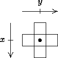
Figure 2-1: The von Neumann neighborhood for an agent at (x, y)

If the selected neighbor agent is fertile and if there is an unoccupied cell (for the child) within the von Neumann neighborhood of either agent, the neighbor agent is a candidate for mating.

Repeat until the candidate agent with maximum wealth is found or the nearest neighbor search is exhausted.

2.9

If a mate is found (i.e., there is at least one candidate agent), the female agent of the pair becomes pregnant. Throughout the gestation period, neither the male nor the female agent can move or attempt to reproduce. The initial endowment of wealth (resource) to the child, equal to the sum of half the initial wealth of each parent, is computed at the time of conception. Attribute inheritance rules for the child agent remain the same as in Epstein and Axtell's model. At the time of birth, the unoccupied cell with maximum resource from the union of the von Neumann neighborhoods of both parents is selected for the child to occupy. If no such cell is available the child dies at the time of birth³.

Model Time Evolution

3.1

Although given little consideration in most artificial society discrete-event simulation models, time evolution is an important part of our research. We agree that synchronous time evolution may be appropriate in some artificial society models if, for example, movement is seasonally motivated. However, many other models are more accurately modeled using asynchronous time evolution. In general, we claim that the use of asynchronous time evolution yields a more realistic simulation model and minimizes simulation artifacts.

Synchronous Time Evolution

3.2

Synchronous time evolution involves fixed-increment time steps, with time conventionally denoted t = 0, 1, 2,  , T. All events of interest must occur precisely at these time steps. For instance, in the Epstein and Axtell model all agents attempt to move simultaneously, once each time step. All agents attempting to reproduce must also do so once each time step. For serial program execution, this kind of parallel activity is not possible and so it is necessary to randomize the order in which agents act at each time step. Without this randomization, the agents will always act in the same order, introducing a bias that can produce artifacts (Epstein and Axtell, 1996).

3.3

Given the model attribute T, which defines the number of simulated time steps, the artificial society model evolves synchronously in time according to the following pseudocode algorithm.

  /* initialize the landscape */
  /* initialize the agents    */
  t = 0;
  while (t <= T) {
    /* move and reproduce the agents      */
    /* update the landscape               */
    /* update the agent list              */
    /* randomize (shuffle) the agent list */
    t++;
  }

Algorithm 3-1: Synchronous time evolution algorithm

3.4

Note the ambiguity in the order of events inside the while loop. For example, should the landscape be updated before or after the agents move?

Asynchronous Time Evolution

3.5

Asynchronous time evolution allows each type of event to occur at random at its own characteristic rate. In this way, individual agent movement events and reproduction events occur at distinct times. That is, whereas the order of agent actions must be specifically randomized at each time step in the synchronous case, randomization is inherent in the asynchronous case. In addition, in the asynchronous case there is no ambiguity in the order of events.

3.6

To facilitate asynchronous time evolution, we construct our artificial society model using the next-event simulation approach. For a next-event simulation model, we must clearly define the system state, the event types, the simulation clock, and a set of algorithms for each event type that define the state changes that occur when each type of event occurs (Park and Leemis, 1999).

3.7

The simulation clock is the real-valued global time parameter t. As defined in ¶2.3, at any time 0 t T, the state of the system is defined by the following set of variables⁴.

• A(t);
  
  
• o(x, y, t) and r(x, y, t) and d(x, y) for all (x, y) ;
  
  
• (x, y)_a and w_a(t) and m_a(t) for all a = 0, 1,  , A(t) - 1.

3.8

Accordingly, there are four types of events that can change the state of the system.

• Movement and corresponding resource consumption by agent a will change (x, y)_a and w_a(t) for the agent, o(x, y, t) and r(x, y, t) for the departed and newly occupied landscape cells, and d(x, y) for the departed landscape cell.
  
  
• The death of agent a will change A(t), and o(x, y, t) and d(x, y) for (x, y)_a.
  
  
• A successful mating by an agent a with another agent a' will change m_a(t) and m_a'(t) for the agents.
  
  
• The birth of a new agent a" from parent agents a and a' will change w_a(t) and w_a'(t), m_a(t) and m_a'(t). If there is an unoccupied landscape cell for the new agent to occupy, the birth will change A(t), create (x, y)_a" and w_a"(t), and change o(x, y, t) and r(x, y, t) for (x, y)_a".

3.9

Because there is a gestation period, the state of the system can change when agents mate and when a new agent is born. For this reason, the reproduction rule, as defined in ¶2.8, is modeled by two distinct types of events. A mating event type initiates the gestation period if the female agent becomes pregnant. Since a mating event is an attempt to reproduce, the mating event does not guarantee pregnancy. A birth event type signals the end of the gestation period when the new agent is born (if possible). Both of these event types can change the state of the system as described above.

Asynchronous Inter-Event Times

3.10

For each event type, inter-event times are assumed to be iid Exponential (1 / ) where is the rate of occurrence of that event type. Equivalently, each event type is modeled as a stationary Poisson process with rate . The Poisson rate for the agent movement process is = 1.0 ⁵. The mating event type can either be coupled with the movement/consumption event type or modeled as a separate stationary Poisson process. If the two event types are coupled, a mating event occurs for an agent each time a movement/consumption event occurs for that agent. For all the results in this paper, if the two event types are uncoupled, the Poisson rate for agent mating is also = 1.0.

Asynchronous Resource Regrowth

3.11

Resource regrowth is not considered an event, but rather an inherent part of the other events. At t = 0 the resource level at each (x, y) cell is the same as the resource capacity at that cell. As time evolves, the cell resources are depleted only when an agent occupies a cell. While the cell remains occupied, the resources continue to grow, but are continuously gathered by the occupying agent; at the moment an agent departs, the cell has no resources. As time evolves, the cell resources can then regrow up to the resource capacity at the cell, provided the cell does not become occupied again. Because the onset of regrowth is a direct result of the interaction of an agent with a landscape cell, we include regrowth as part of the movement, mating, and birth events.

3.12

For each (x, y) landscape cell, as time evolves d(x, y) is defined by the last time an agent departed that cell. At time t > d(x, y), we can compute the current level of resource at cell (x, y) by the equation

r(x, y, t) = min{ (x, y),  (x, y)(t - d(x, y)) }.

Asynchronous Time Evolution Algorithm

3.13

Given T, the artificial society model evolves asynchronously in time according to the following pseudocode algorithm. The algorithm presumes the existence of a procedure GetNextEvent() that returns the event time and event type of the next (most imminent) event.

  /* initialize the landscape */
  /* initialize the agents    */
  t = 0.0;
  while (t <= T && A > 0) {
    event = GetNextEvent();
    t = event.time;
    switch (event.type) {
      case movement:
        /* unoccupy the current cell */
        /* select the (x,y) cell within the FOV with maximum resource */
        /* occupy the selected (x,y) cell */
        /* update the wealth of the agent */
        /* schedule the next movement event */
      case death:
        A(t)--;
        /* unoccupy the current cell */
      case mating:
        /* execute the mating algorithm */
        if ( /* the mating is successful */ ) {
          /* compute endowments and update the wealths of the parents */
          /* update the mate pointers of each parent */
          /* schedule a birth event */
          /* cancel any parent agent events to occur before the birth */
        }
      case birth:
        /* update the wealths of the parent agents */
        /* schedule the next event occurrences for each parent agent */
        if ( /* there is an (x,y) cell for the new agent */ ) {
          A(t)++;
          /* initialize the new agent */
          /* occupy the selected (x,y) cell with the new agent */
          /* update the wealth of the new agent */
          /* schedule the next event occurrences for the new agent */
        }
    }
  }

Algorithm 3-2: Asynchronous time evolution algorithm

Synchronous Time Evolution Via Next-Event Simulation

3.14

For the purpose of using one program to compare synchronous and asynchronous time evolution, an attractive alternative to Algorithm 3-1 is to implement synchronous time evolution using next-event simulation, similar to Algorithm 3-2. Except for the timing results in Figure 5-2, this is the approach we use for the results presented herein. The system state, event types, simulation clock and set of algorithms described for the asynchronous model remain the same. However, different event types no longer run as Poisson processes with their own characteristic rates. Instead, we implement the simultaneous occurrence of synchronous events at fixed time steps by forcing agent events to occur at random within a small window at times t, t + 1,   as shown in Figure 3-1 where bullets denote typical agent events.

Figure 3-1: Next-event simulation of synchronous events

3.15

The movement/consumption and mating events for an agent occur at the same time. Birth and/or death events, if they are to occur, also take place at this time.

Results

4.1

The goal of the work by Epstein and Axtell (1996) was to examine collective social behavior by using a discrete-event simulation model based on simple rules and initial configurations. Our focus is on the implementation of the simulation model rather than the development of new artificial society models or the social interpretation of the results produced by these models. With this motivation, we now provide results from the artificial society model defined in Section 2 to support our claim that, based on the choice of asynchronous or synchronous time evolution, very different behavior can be observed in the resulting output.

4.2

The following figures were motivated by an attempt to replicate the results Epstein and Axtell obtained when combining agent movement with reproduction. Despite considerable experimentation, we were never able to reproduce the results in Figure III-4 (Epstein and Axtell, 1996). Since Epstein and Axtell never reveal their model for the landscape capacity (perhaps for brevity), there is some uncertainty in our choice of (x, y). However, we conjecture that the oscillatory behavior shown in Figure III-4 is a simulation artifact caused primarily by synchronous time evolution. Moreover, this oscillatory behavior is very much dependent upon initial conditions which to date we have been unable to determine.

Mating Tied to Movement

4.3

For Figure 4-1, we used an X    Y = 50    50 landscape. The resource capacity at each cell is given by the equation in ¶ 2.6, and the resource growback rate for each (x, y) cell is (x, y) = 1. The landscape is initially occupied with A(0) = 400 randomly placed agents. The initial wealth of each agent is w(0) = 10. The attributes for each agent are initialized as random variates according to⁶

:	Equilikely(1, 6);
:	Uniform(1, 4);
:	Uniform(60, 100);
:	Uniform(12, 15);
:	Uniform(40, 50) for females, Uniform(50, 60) for males.

The agents execute the movement/consumption and reproduction rules, with = 0. Reproduction and movement are coupled, i.e., the mating event type is not modeled as a separate process.

4.4

Figure 4-1 depicts the time evolution of the agent population for five different initial random number generator seeds with T = 2500. In general, the output produced using synchronous time evolution is the more oscillatory of the two curves, while asynchronous time evolution produces the more stable darker curves. Epstein and Axtell propose explanations of the large oscillatory behavior in terms of population dynamics. Although in a few atypical cases asynchronous time evolution produced large oscillations in the population⁷, we believe that, in general, the large oscillations produced by Epstein and Axtell are simulation artifacts produced by the use of synchronous time evolution.

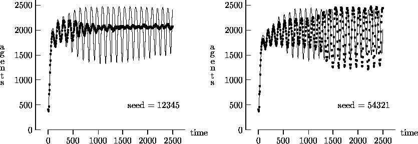
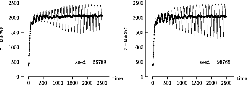
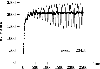
Figure 4-1: Asynchronous vs. synchronous time evolution, 50    50 landscape

4.5

Figure 4-2 depicts the time evolution of the agent population for an X    Y = 100    100 landscape with an initial A(0) = 1600 randomly placed agents. The remaining state and attribute parameters are the same as in Figure 4-1. Again, undamped oscillatory behavior is present in the synchronous time evolution output but not in the asynchronous time evolution output⁸. While some initial oscillation is present in the asynchronous time evolution results, the amplitude is damped considerably. Moreover, for all initial seeds, changes in the output are far less dramatic in the asynchronous case. That is, unlike the synchronous results, the asynchronous results are not sensitive to the random variate sequence of movement and reproduction, as manifested by the choice of initial seed.

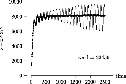
Figure 4-2: Asynchronous vs. synchronous time evolution, 100    100 landscape

4.6

We felt that T = 2500, as suggested by Epstein and Axtell, may not yield a sufficient measure of the long-term time evolution of the agent population. For this reason, Figure 4-3 depicts the time evolution for the same initial conditions as Figure 4-1, but with T = 25,000. In these figures, the highly oscillatory behavior of the synchronous time evolution output persists, while the asynchronous time evolution produces a stable agent population in virtually all cases.

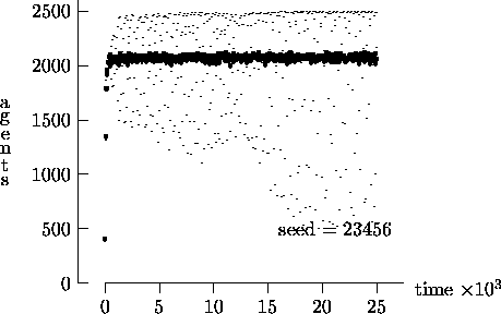
Figure 4-3: Asynchronous vs. synchronous time evolution, 50    50 landscape

4.7

Similarly, Figure 4-4 depicts the time evolution for the same initial conditions as Figure 4-2, but with T = 25,000. In this figure, we see the oscillatory behavior persisting in a majority of the synchronous time evolution output. In contrast, the asynchronous time evolution quickly produces a stable agent population. We present the results in Figures 4-1, 4-2, 4-3 and 4-4 as strong evidence that very different behavior can result from the choice of modeling time evolution as synchronous or asynchronous.

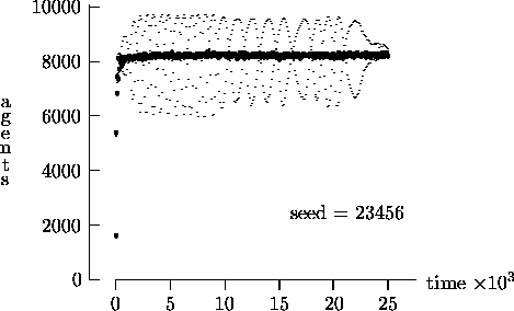
Figure 4-4: Asynchronous vs. synchronous time evolution, 100    100 landscape

Mating Modeled Separately

4.8

For the results in Figure 4-5, the mating event type is no longer coupled with movement but is modeled as a separate Poisson process as described in ¶ 3.10. Otherwise, everything is the same as in Figure 4-1, with the exception that = 1. Again, the darker curves represent output from the asynchronous time evolution model. We see that not only is the amplitude of oscillations diminished dramatically using asynchronous time evolution, but when compared with Figure 4-1 the mean of the agent population is lowered as well. We reemphasize that we are not promoting asynchronous time evolution as the best approach for all artificial society models, but these results show that very different output can result from modeling time evolution as synchronous or asynchronous.

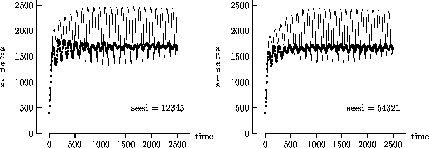
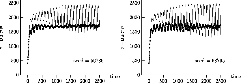
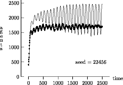
Figure 4-5: Asynchronous vs. synchronous time evolution, mating uncoupled

Computational Performance Issues

5.1

Although asynchronous time evolution in an artificial society discrete-event simulation model can reduce simulation artifacts and sensitivity to initial conditions, computational performance can suffer significantly unless the next-event approach is implemented properly. In this section we provide a discussion of two possible algorithms and data structures for handling the associated event list. We also demonstrate that acceptable computational performance can be achieved by a judicious choice of the event list implementation.

An Initial Event List Approach

5.2

The asynchronous time evolution in the next-event simulation of the artificial society model is driven by an event list. Each element in the event list is associated with the future occurrence of a single event, where the type of that event is exactly one of the four event types defined in ¶ 3.8. For the artificial society model, each element in the event list contains the time that the associated event is to occur, the type of event, and a pointer to the corresponding agent.

5.3

Given that each agent can execute only one type of event at a time, we can simplify the event list by including only the most imminent event for each agent. In this way, there is one event per agent in the event list. Since the type of the most imminent event for each agent can be determined from the agent data structure, we no longer need the type of the event in the event list. If we use a singly-linked list data structure to represent the event list and sort the events by increasing time of occurrence, we obtain a sample event list like the one shown in Figure 5-1.

Figure 5-1: A typical event list for the artificial society model simulation

5.4

Using this approach, the next event to occur in simulated time is always the first element in the linked list. In this way, the GetNextEvent() procedure from Algorithm 3-2 is implemented by simply returning the head of the linked list. However, when a new event is inserted into the event list, a linear search must be executed from the head of the list to determine the appropriate insertion point. Similarly, any search for a canceled event also requires a linear search. For a large number of events, i.e., as the number of agents grows, such linear searches seriously degrade the computational performance of the simulation.

5.5

Figure 5-2 depicts sample execution times⁹ for a standard synchronous implementation of the artificial society model and an asynchronous implementation using the previously described singly-linked list event list approach. Each value displayed is the average time for five replications along with the corresponding 95% confidence interval. The simulation was executed with T = 500 for the increasing landscape sizes shown, each initially populated with 16% agents¹⁰. The initial values for agent states and attributes were the same as described in ¶ 4.3, except initial agent wealth was w(0) = 25. Agents were not permitted to reproduce so that the number of agents monotonically decreased for the duration of the simulation. As shown, as the initial number of agents increases (with landscape size), the performance of the sorted linked list implementation degrades quickly.

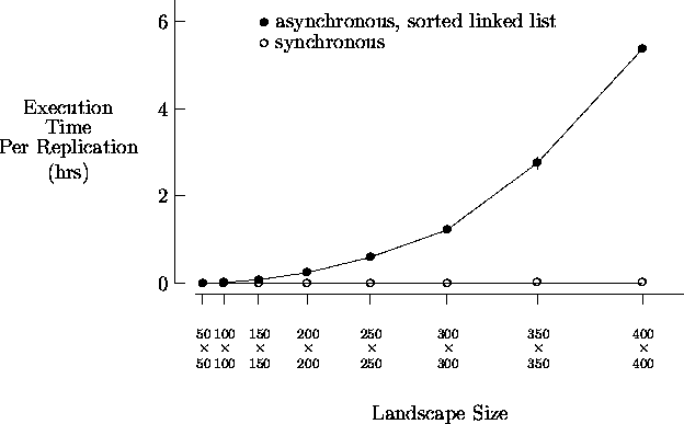
Figure 5-2: Sample execution times

An Improved Event List Approach

5.6

To improve upon the sorted singly-linked list approach described in the previous section, an alternate approach is needed. Of the possible event list algorithms available, Henriksen's algorithm (1977, 1983) is a natural extension to the sorted linked list approach. As shown in Figure 5-3, the linked list is modified to be doubly-linked and includes "dummy" low and high events at the respective ends. Similar to the previous approach, retrieving the next event to occur in simulated time, always the second element in the linked list, remains a simple operation.

5.7

As depicted in Figure 5-3, a linear search is avoided through the use of an auxiliary search array. Each element in the search array contains an event time and a pointer to an event in the event list. The search array is sorted by decreasing event time. A typical binary search of the search array, a variation on Henriksen's approach, is used to find the smallest time in the search array greater than the event time sought. Beginning with the event pointed to by the selected search array element, a linear search of the event list in descending order ensues until the desired event time is found. During the binary search, Henriksen's "pull" technique (1983) is used to keep the search array pointers evenly distributed throughout the event list. The end of the search array is maintained, and the size of the array is increased if necessary¹¹.

Figure 5-3: The typical event list improved with search array

5.8

Figure 5-4 depicts sample execution times for an asynchronous implementation of the artificial society model using the sorted linked list approach and the modified Henriksen's approach. Again, each value shown is the average time for five replications along with the corresponding 95% confidence interval. The simulation was executed with T = 500 for the increasing landscape sizes shown, each initially populated with 16% agents. As shown, the data structure and algorithm modifications used in the modified Henriksen's approach yield execution times comparable to those of the standard synchronous implementation given in Figure 5-2. Also shown are the times obtained using the modified Henriksen's approach with agents able to reproduce. Although the number of agents is no longer monotonically decreasing (in time) in this case, acceptable performance is still achieved. These results show that when implemented properly, the loss in computational performance resulting from the use of asynchronous time evolution is minimal in a typical artificial society discrete-event simulation.

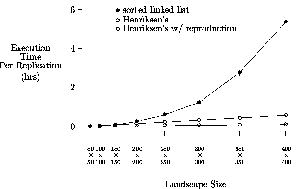
Figure 5-4: Sample execution times

Conclusions and Future Work

6.1

For applications involving natural asynchronous behavior, time evolution in an artificial society discrete-event simulation model is more appropriately modeled asynchronously rather than with the typical synchronous approach. In a typical artificial society model adapted from Epstein and Axtell, asynchronous time evolution produces output that is very different from output obtained using synchronous time evolution. Specifically, the use of asynchronous time evolution reduces simulation artifacts and sensitivity to initial conditions.

6.2

Asynchronous time evolution is implemented using a next-event simulation approach. If implemented poorly, a next-event artificial society simulation model can suffer dramatically in terms of execution time. However, through the use of proper event list data structures and algorithms, execution times are comparable to those of a typical synchronous time implementation.

6.3

The results in this paper suggest that when judiciously implemented, asynchronous time evolution in an artificial society discrete-event simulation model is an attractive alternative to synchronous time evolution in terms of both the quality of the resulting output and computational performance. Future work involves the systematic study of both standard and novel event list data structures and algorithms on a more comprehensive artificial society model. We also plan to investigate various approaches for executing the artificial society simulation in parallel.

Appendix: Random Variable Models

The following material was taken directly from Park and Leemis (1999). A random variate is an algorithmically generated realization of a random variable. The purpose of this appendix is to provide definitions of the random variable models used to generate the Uniform, Exponential and Equilikely random variates from ¶ 3.5, 3.10 and 4.3¹².

Uniform

The continuous random variable X is Uniform(a, b) if and only if

• the real-valued parameters a, b satisfy a < b
  
  
• the possible values of X are = { x | a < x < b }
  
  
• the probability density function of X is
  
  
  as illustrated
  
  
  
• the mean of X is
  
  
  
  
• the standard deviation of X is
  
  
  
  

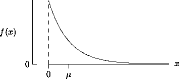
Exponential

The continuous random variable X is Exponential( ) if and only if

• the real-valued parameter   satisfies > 0
  
  
• the possible values of X are = { x | x > 0}
  
  
• the probability density function of X is
  
  
  as illustrated
  
  
  
• the mean of X is  
  
  
• the standard deviation of X is
  
  
  
  

Equilikely

The discrete random variable X is Equilikely(a, b) if and only if

• the parameters a, b are integers with a < b
  
  
• the possible values of X are = {a, a + 1,  , b}
  
  
• the probability density function of X is
  
  
  as illustrated
  
  
  
• the mean of X is
  
  
  
  
• the standard deviation of X is
  
  
  
  

Notes

¹ For means of comparing asynchronous with synchronous time evolution, the next-event implementation is easily modifiable to simulate synchronous time evolution.

² If the gestation period is = 0, the behavior of agents under our reproduction rule is the same as if the gestation period was omitted from the rule.

³ If > 0, during the gestation period other agents may occupy all the cells adjacent to the parents. Consequently, at the time of birth a cell may not be available for the child to occupy.

⁴ For convenience, the state description includes some variables that could be determined from other variables. For instance, A(t) can be determined by summing o(x, y, t) for all (x, y) . Accordingly, the state description is not minimal.

⁵ It is common to assume that a stochastic process which occurs "at random" is a stationary Poisson process. The Poisson rate = 1.0 corresponds to the fixed-increment time step rate of the synchronous approach. Systematically increasing produces time evolutions similar to those presented in Section 4 but with lower population means. We also experimented with inter-event times as Uniform, Erlang and Normal random variables, each with a mean of 1.0 (the Normal was truncated to positive values). These other distributions for the inter-event times produce results similar to the stationary Poisson process results.

⁶ An Equilikely random variate is the discrete analog of a continuous Uniform random variate (Park and Leemis, 1999).

⁷ The oscillatory behavior associated with the initial seed 54321 never diminished. Instead, the population swings eventually led to termination at approximately t = 45,000. We consider this atypical case an outlier since we were able to produce similar results only four times using 100 different initial seeds.

⁸ Unlike the 50    50 landscape results, asynchronous time evolution produced no atypical behavior in any of the results using 100 different initial seeds on a 100    100 landscape. To date we have not performed a more systematic study of this atypical behavior in either the 50    50 or 100    100 landscape case.

⁹ All timing results were obtained using a dedicated Pentium II 350 MHz processor with 128 MB of RAM.

¹⁰ The effect of landscape size on execution time is negligible. Nearly identical timings were obtained when the landscape size was increased but the initial number of agents remained constant.

¹¹ We initially allocate a dynamic search array of size 1024. The end of the search array is determined by the number of valid entries in the array. When necessary, the size of the search array is systematically doubled.

¹² In the definitions to follow, the use of to represent the mean and to represent the standard deviation is consistent with conventional statistical notation and is not to be confused with the and notations from ¶ 2.7.

References

EPSTEIN, Joshua M. and Robert Axtell. 1996. Growing Artificial Societies. Brookings Institution Press, Washington, D.C.

HENRIKSEN, J. O. 1977. An improved event list algorithm. In Proceedings of the Winter Simulation Conference, pages 547-557.

HENRIKSEN, J. O. 1983. Event list management -- a tutorial. In Roberts, S., Banks, J., and Schmeiser, B., editors, Proceedings of the 1983 Winter Simulation Conference, pages 542-551. IEEE.

MÜLLER, H. J., T. Malsch and I. Shulz-Schaeffer. 1998. Socionics: Introduction and potential. Journal of Artificial Societies and Social Simulation, 1(3), https://www.jasss.org/1/3/5.html.

PARK, Steve and Larry Leemis. 1999. Discrete-Event Simulation: A First Course. College of William and Mary, Williamsburg, VA.

Return to Contents of this issue

© Copyright Journal of Artificial Societies and Social Simulation, 1999