© Copyright JASSS

  JASSS logo ----

Günter Haag and Philipp Liedl (2001)

Modelling and Simulating Innovation Behaviour within Micro-based Correlated Decision Processes

Journal of Artificial Societies and Social Simulation vol. 4, no. 3,
<https://www.jasss.org/4/3/3.html>

To cite articles published in the Journal of Artificial Societies and Social Simulation, please reference the above information and include paragraph numbers if necessary

Received: 5-Oct-00      Accepted: 13-Mar-01      Published: 30-Jun-01


* Abstract

The economic evolution and production has been subject to major shocks and structural changes during the last decades. Beside the standard production factors such as the capital and labour force new production factors for taking into account technological progress and knowledge production and knowledge transfer have to be considered.

Modelling of the evolution of technologies as well as structural changes in the management of firms however, require a better understanding of knowledge production and the knowledge transfer process within and between industries, the role and efficiency of transfer institutions such as universities, technology-transfer centres and consulting companies. The paper aims to provide a decision-based framework for this kind of complex interwoven processes.

Keywords:
Innovation, Spillover effects, Decision processes, Knowledge accumulation, Technology transfer

* Introduction

1.1
In neoclassical theory of economic growth innovations are viewed as being exogenous. Technological progress is treated in production functions as a shift parameter. This view cannot explain the causes of technical progress and it is unsuited to study the impact of a varying rate of technical change (Jungmittag et al. 1999). Furthermore interactions of firms using different technologies are not considered. The assumption of economic equilibrium in the neoclassical point of view is inconsistent with Schumpeter´s concept of the creative entrepreneur (Schumpeter 1934), because once equilibrium is reached no agent of the economic system can leave this due to optimal decision making.

1.2
This work was guided by the insufficiencies mentioned above and since R&D-expenditures have been identified as one of the most important determinants for the development of markets. Market results are not only determined by the ratio of prices and marginal costs, but also by the rate of technical change and the variety of products (Audretsch 1996).

1.3
During the last decades several approaches have been made to describe the effect of knowledge and innovations on the success of firms apart from the exogenous view of neoclassical theory. Some of them will be summarised in the following paragraphs.

1.4
The first approach to treat technological progress as an endogenous process was made by Arrow (1962). He regarded technological progress as an experience of firms due to learning by doing. In this respect technological progress is a by-product of investment, so the innovation process is not depicted directly (Pyka 1999).

1.5
Recently an important approach towards the modelling of innovations is using game theory to simulate the behaviour of the innovation system (Audretsch 1996). In this context studies on license-agreements and adoption of innovations have been carried out. Examples of a game theoretical approach are given by v. Hippel (1989) and Witt (1995). They both use the prisoners dilemma to describe the conflicting situation in which a firm has to decide whether to exchange knowledge with another firm or not.

1.6
In their fundamental work Nelson and Winter (1982) have suggested another way of view referred to innovations. They use an evolutionary model to describe changes in the behaviour of firms with respect to the development of new techniques. They call all regular and predictable behavioural patterns of firms routines. Changes in those routines are made by searching for new rules. Stochastic elements are used to model uncertainty of the outcome of research activities.

1.7
In this context Pyka (1999) emphasised the importance of interactions between firms. In his model firms can participate in so called informal networks as introduced by v. Hippel (1989). The members of those networks exchange new techniques voluntarily. This leads to the view of a collective innovation process, were all economic agents can benefit of new techniques and technologies developed by other members of the network. One important condition for these technology "absorbing" firms consists in the available knowledge they already have to use the new technique of their own. In this sense spillovers are interpreted to have a positive effect for those firms being members of the informal network, since R&D investments for parallel- or multi-development of one and the same technique can be saved.

1.8
It is the aim of this paper to provide a decision-based framework for the complex and interwoven processes of production and innovation, labour force and capital formation as well as knowledge production and knowledge transfer processes within and between industries including the role and efficiency of transfer institutions. Thus the master equation framework is used to model and simulate the decision behaviour of firms (entrepreneurs) to shift their overall business strategies.

1.9
The framework of the master equation approach is a fundamental tool for describing the dynamics of probability distributions related to a multiplicity of interacting economic agents. This equation has its roots in statistical physics and was first applied to sociology and economics by Weidlich and Haag (1983).

1.10
The master equation is applied in Cantner and Pyka (1998) to describe probability distributions of a large amount of agents either to express technological changes or changes in behavioral patterns of firms, i. e. weather to cooperate with other firms or not (Pyka 1999) or to develop new products or not (Woeckener 1993).

1.11
The interaction of knowledge creation with standard capital formation in an economy is considered in Andersson (1981) and Andersson and Matsinen (1980). However, it provides considerable difficulties to estimate the stock of knowledge and its depreciation rates in a reasonable and acceptable way.

1.12
Furthermore, the volume of R&D spent in the production process as well as the know how transfer from research institutions or universities, from consultants or transfer institutions like the Steinbeis-Institutes are essential parts within the innovation process for new products or production processes. This means that knowledge has - at least partially - a public goods character, in that it may participate as an input in the production process without being used. On the other hand, knowledge acquisition, information retrieval, knowledge transfers etc. requires time, efforts and costs. Consequently these processes have to be considered within the open space of firms strategic decisions.

1.13
In this paper we follow the approach of Haag (1989) and Müller and Haag (1996). In this concept the classical input factor labour is "enhanced" by transfers of technologies from the economic and the scientific system. The accumulation of labour and knowledge-transfers is called know-do (Müller and Haag 1996). The idea of the know-do concept is that research co-operations within the economic system require a specific amount of working hours in other firms and co-patenting activities with a university demands a certain amount of time in the scientific area. So the efforts spent in knowledge transfers can be measured in working hours.

1.14
Outsourcing the development of new technologies gives firms the advantage of using these technologies without the necessity to employ workers for doing the development of their own, so there are positive effects of transferring know-how.

1.15
Before we start with the development of our macro-economic model we have to define what is meant by the word innovation. We will use the definition of the OECD and Eurostat given in the Oslo-Manual (OECD and Eurostat 1997):
Technological product and process (TPP) innovations comprise implemented technologically new products and processes and significant technological improvements in products and processes. A TPP innovation has been implemented if it has been introduced on the market (product innovation) or used within a production process (process innovation). TPP innovations involve a series of scientific, technological, organisational, financial and commercial activities. The TPP innovating firm is one that has implemented technologically new or significantly technologically improved products or processes during the period under review.
The term product innovation on the one hand includes technologically new products whose technological characteristics or intended uses differ significantly from those of previously produced products and on the other hand technologically improved products which means that the performance of an existing product is significantly enhanced or upgraded (OECD/Eurostat 1997).
A process innovation is the adoption of technologically new or significantly improved production methods, including product delivery. These methods may be intended to produce or deliver technologically new or improved products, which cannot be produced or delivered using conventional production methods, or essentially to increase the production or delivery efficiency of existing products. (OECD/Eurostat 1997).
1.16
At this point one has to distinguish between innovations and inventions. Inventions are not necessarily implemented in terms of the OECD definition quoted above. Only inventions that are implemented to products or processes are called innovations.

1.17
Furthermore, it is important in this context to distinguish between knowledge and information. The term knowledge is commonly used to describe research results that are difficult to codify such as tacit knowledge (Nelson and Winter 1982) and hence difficult to transfer between participants of a network of innovating firms (Teece 1998). To describe data that is easy to codify and thus easy to transfer, the term information is used. Thus, information involves all messages and routinised data that is not tacit respectively not too complex to codify and to store (Kobayashi et al. 1993).

1.18
The paper is organised as follows: In section 2 the macro-model of the nested innovation process will be introduced. Numerical simulations of interacting firms will be presented in section 3. The variety of possible solution pattern including limit cycles and deterministic chaos and the related stability considerations exhibit the dangerous trajectories of firms between of being exhausted or in a growing phase.

* Modelling of Nested Innovation Processes

The Inter-linked Network of Firms

2.1
In this section we will develop an appropriate complex macro-model of the nested innovation processes of a network of firms which avoids some shortcomings of earlier knowledge based concepts (Haag 1989, Müller and Haag 1996).

2.2
As empirical studies show (Fischer and Menschik 1994), there are internal and external impulses for firms to innovate. Internal impulses come from the research and development the firms do on their own and from decisions of the management. External impulses are arising from observing the competitors and their products, from trade fairs or product shows and congresses and from contacts to universities and research centers. So an appropriate model simulating innovation processes in a firm should include besides own R&D activities the impacts of other firms as well as influences from the scientific system.

2.3
The term scientific system includes both universities, research institutes, technology consulting agencies and technology transfer centers like the Steinbeis Transfer Centers.

2.4
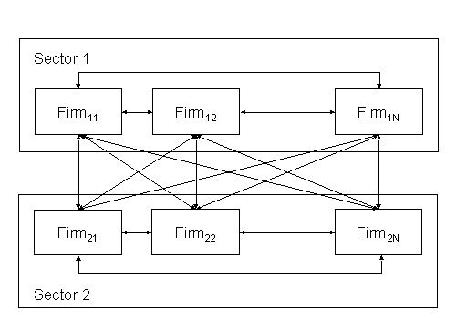
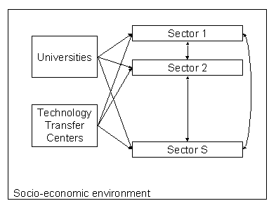
In order to describe the impact of different transfer activities on the production of a specific firm, the notion of spillover effects (inter-firm as well as intra-firm spillovers and transfers between the scientific system and the firms) is commonly used. First the impact of spillover effects on the evolution of inter-linked firms or companies will be examined. Therefore, a network of interacting firms belonging to one or several sectors is considered. This network is illustrated together with the linkages to the scientific system in Figure 1.

Fig 1
Figure 1. Nested system of economic agent

2.5
The interactions of the firms will be determined by the impacts of spillover effects. Competition of the different firms on the market is not explicitly modelled in this introductory part. Nevertheless the impacts of spillover effects on the firms depend on their co-operation and competition strategies.

2.6
The spillover effects thus may have both positive and negative impacts on the economic development of a firm.

2.7
Spillover effects having positive impact can be identified if in one sector e.g. a process innovation has a positive impact on the production of other sectors. The product innovations of one sector may be very important for the development of new products or processes in another sector. Such a positive network effect may lead to a significant increase in production of a sector. For example, the developments in the semiconductor industry has lead to a reduction in size of electronic components used by the computer industry for their own products. This reduction was necessary to allow the computer industry to produce small personal computers for private consumers.

2.8
On the other hand spillover effects having negative impact may be observed if one innovation in a specific sector has an negative impact on the development of new products or processes in another sector. Silverberg and Lehnert (1994) give an example for such a negative effect between sectors: On primary energy sector, wood and coal have been replaced by oil and nuclear power during the 20th century, and with them the machinery that is necessary to transform these energy sources into electric power.

2.9
Firms belonging to the same sector may in principle interact with other firms of the same and other sectors as illustrated in Figure 2. Within one sector the competition for the most advanced products (high-tech products) is responsible for spillover effects with respect to product innovations (Pyka 1999). Process innovations are introduced mainly to reduce costs of production and to enhance the quality of products (Fischer and Menschik 1994).

Fig 2
Figure 2. Interdependencies of firms belonging to two industrial sectors

2.10
An example for a spillover effect having positive and negative impact within one sector is the imitation of one firm's innovations by others. The economic impacts for imitating firms are positive since they benefit from the technologies developed by the innovating firm without doing the whole research and development of their own. On the other hand the innovating firm experiences negative impact of this spillover effect caused by the imitating firms, because with the spread of the innovation on the market the firm innovating first loses market shares to the imitating firms. So imitation reduces the economic benefits of an innovation due to negative network effects.

2.11
An example of a spillover effect having a negative impact is the complete replacement of the video-recording system Betamax, introduced by Sony in 1975, by the VHS-system of JVC (Arthur 1989, Woeckener 1995).

2.12
A possible co-operation of two firms may lead to positive spillover effects for both of them since costs for multi-development of one and the same innovation can be saved (v. Hippel 1988, Pyka 1999).

2.13
Imitation as well as co-operation strategies are causing diffusion of innovations in the economic system. Such innovation diffusion processes are described among others by Pyka (1999) or Maier (1998).

2.14
Due to the fact, that spillover effects are occurring between firms of different sectors as well as between firms of the same sector it is sufficient to introduce only one multiple index in order to describe the firms position within the innovation network.

Modelling of the Macro-Economic Network of Inter-Linked Firms

2.15
In the following the model will be formulated in mathematical terms. The focus will be on the supply side of the market. Besides spillover effects in the innovation sector described above and innovation efforts of the firms under consideration, the production and consequently the economic development will depend on the classical factors capital and labour. Decisions of investments will be made by the firms with respect to profit maximisation. In order to describe the production of the individual firms, taking into account the impact of spillover effects, we will not follow the concepts of Lucas (1988) and Romer (1986) who take the human capital of a society, respectively the results of R&D of the whole economy into account, for describing spillover effects. As mentioned by Romer (1990), the major problem of these models are, that the entire stock of knowledge is regarded as a public good.

2.16
We will assign each firm i a production function of the form Qi = f(Ki, Li, Ii). So we make a distinction in input factors between the capital stock Ki of the firm i, labour force Li and the impact of innovations Ii. We choose a modified Cobb-Douglas production function:[1]

eqn 1 (1)

This means Ii is that part of a mixture of knowledge, innovation and information used by firm i in its production process, whereby the parameter b describes the efficiency of using this mixture for production. Thus, Ii covers knowledge and information with public good character as well as without. Spillover effects will be modelled within Ii and not directly in the production function.

2.17
For simplicity it is assumed that only one product is produced. Moreover we assume that the elasticities of production α1 and α2 as well as the scaling factor a are the same for all firms.

2.18
The variable for innovation activity Ii contains the impact of innovations on the firms output developed by firm i itself and innovations from other firms and from the scientific system. Therefore, positive or negative effect on firm i due to spillover effects may be observed.

2.19
The assignment of innovations to the classical production factor labour has been described by Müller and Haag (1996). Because of the difficulty of estimating the impact of innovations a new production factor called know-do Di was introduced. Aside intra-firm labour all inputs like inter-firm innovation transfers, intra-firm research and development and inputs of e.g. universities or transfer institutes can be measured in terms of working hours. Introducing know-do to our model we have:

eqn 2 (2)

In case of Ii = 0, i.e. if firm i is not innovating and there are no innovation or technology transfers from outside the firm, the chosen production function (1) becomes the neoclassical Cobb-Douglas production function.
2.20
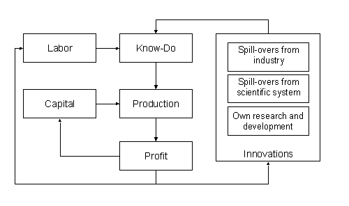
In Figure 3 we give a schematic overview of the model in case of one firm.

Fig 3
Figure 3. Graphical description of the innovation process in case of one firm

2.21
The three input factors capital stock Ki, labour force Li and innovation activity Ii can be increased by investments Yi. In neoclassical models, investments are often assumed to be Yi = siQi, with a constant rate of savings si (Gandolfo 1980). We assume that for large production investments are increasing with smaller rates than for small production. The reason is that with increasing size of investment projects it becomes more difficult for the firms to realise these projects. For example the construction of a whole factory is limited by the area useable for production and limited by the time needed to build the factory. So investments that can be realised in one production period are limited. Besides this structural limitation of investment it is not appropriate for the firms to invest more in production than for the satisfaction of demand is necessary. For these reasons we assume that investments realised in one production period are limited by a maximal amount of investments Yimax. A simple formulation of the investments Yi modified by this maximal investments Yimax reads:

Eqn 3 (3)

with a rate of savings si. The rate of savings is viewed as being constant over time in a first approximation. Of course, the rate of savings has to fulfil the conditions 0 ≤ si ≤ 1. According to Figure 4, for small values of siQi, investments Yi become equal to neoclassical investments Yi = siQi. In the case of very high values of siQi, Yi becomes approximately equal to Yimax.
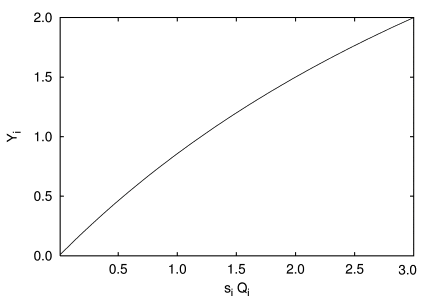
Fig 4
Figure 4. Investments Yi in dependency of siQi with maximal investments of Yimax = 6.0 and a rate of savings si = 0.6

2.22
Continuing in the development of our model, we assume, that firm i can use a fraction of total investments Yi for investing in the three different fields of activity: for increasing the capital stock Ki, investment into labour force Li and investment into innovation activity Ii. So investments Yi will be divided into a part µiKYi that is used for capital accumulation, a part µiLYi that is used for labour formation and a third part µiIYi, used for the formation of innovations. For the ratios of investment µiK, µiL, µiI the following condition has to be satisfied:

Eqn 4 (4)

2.23
The change in time of the capital Ki used for production by firm i is modelled, according to Müller and Haag (1996), via:

Eqn 5 (5)

where δi is the rate of decrease of the capital stock Ki.

2.24
Contrary to neoclassical theory of growth (Solow 1956, Gandolfo 1980) we will not regard labour as being proportional to population. We do not examine the whole economy but the behaviour of individual firms. Therefore we do not assume a direct link between population growth and labour force in the firms under consideration. Rather the demand for labour in the firms will depend besides the wages on their productivity and the overall economic situation. We will thus model labour force endogenously. Let the number of workers Ni employed by firm i be given by:

Eqn 6 (6)

where (i is the rate of decrease of labour force due to natural decreasing factors. This means that investments in labour force are related to the production. If we translate the number of workers in labour hours h afforded in one production period we receive the total labour hours Li used for production in one period:

Eqn 7 (7)

2.25
For the costs of one worker during his employment cN i we obtain

Eqn 8 (8)

where wi is the hourly wage rate and n is the number of production periods a worker is employed.

2.26
With (7) and (8) we receive from (6) the change of labour force with time:

Eqn 9 (9)

2.27
If we formally reduce the length of the employment contracts to the length of one production period, i.e. n = 1, equation (9) yields:

Eqn 10 (10)

2.28
In this approach we assume that the labour market always provides enough workers to the firms. Of course this is realistic in sectors of high unemployment, but not in sectors were qualified labour is rare.

2.29
A similar approach was made by Zhang (1990) and Cigno (1982). In these papers population growth is modelled endogenously in dependence of production. Labour is then, like in neoclassical theory, regarded as being proportional to the population numbers.

2.30
We now turn back to the modelling of innovations. These innovations may be product innovations as well as process innovations. Innovations can have a more ore less continuous character in form of small improvements of products or processes as well as a discrete character in form of radically new products or processes (Freeman 1988). Following the concept of Müller and Haag (1996), we will measure innovations Ii in working hours spent for the development of new products or processes. This concept allows us to regard all innovations as being continuos. We have to consider efforts in research and development within a firm as well as spillover effects from other firms and from the scientific system. The time rate of change in innovation activity Ii is modelled in the following way:

Eqn 11 (11)

where γi is the rate of decrease in innovation activities Ii and accounts for the obsoleteness of older innovations. N is the overall number of firms regarded, M is the number of scientific institutions taken into account.

2.31
We regard, the amount of know-do of firms Dj and scientific facilities Dksci as being responsible for spillover effects. Firm i has access to the labour force Li and innovation activity Ii of other firms e.g. by outsourcing the development of new technologies. This means that the investment into the own labour force and intra-firm research and development can be reduced.

2.32
The factors gij and giksci in (11) are interaction coefficients describing the impact of the spillover effects and transfer activities from other firms and the scientific system. By adequate chosen interaction coefficients the different schemes of interrelated firms or sectors can be described. A simple example is a firm, investing only in own research and development. In this case we have gii > 0, gij = 0, giksci = 0. For a firm using innovations of other firms without investing in own R&D, the coefficients would be gii = 0, gij > 0, giksci = 0.

2.33
The transferability of knowledge and information can be characterised by the value of the interaction coefficients gij and giksci. In principle, one could also assume a dependence of these interaction coefficients on distance of firms when taking regional aspects into account.

2.34
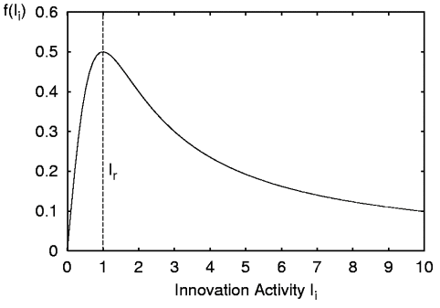
Besides the know-do of other firms Dj and the scientific system Dksci and the corresponding interaction coefficients gij and giksci, the impact of spillover effects on firm i also depend on its own technological level. This is modelled via a spillover function f(Ii). Following Pyka (1999) a firm possessing few knowledge accumulating activities can only take relatively few advantage of innovations produced by other firms, because of lacking experience. On the other hand a firm belonging to the technological frontier has difficulties in increasing its knowledge stock through co-operation with others or even own research and development because of exhausting innovation opportunities. So with increasing innovation activity Ii, the spillover function f(Ii) will increase at first and then at large innovation activity Ii it will decrease. A spillover function that fulfils these requirements reads:

Eqn 12 (12)

2.35
The parameter Ir is needed for scaling the innovation activity Ii. The shape of this function is depicted in Figure 5.

Fig 5
Figure 5. The spillover-function f(Ii) in dependency of innovation activity Ii with a scaling parameter Ir=1 [1/h].

2.36
Of course different functional forms of f(Ii) can be used. However, the general results are not affected by the specific form of (12).

2.37
At next we will take a look on decision processes of firms. Besides decisions concerning marketing strategies and co-operation strategies that are not modelled in this article one important point regarding the production of firms is the decision of firm i to split up the total investments Yi into the three parts: capital stock Ki, labour force Li and innovation activity Ii. As criteria in the decision making process we will use profit maximising rules. The profit πi of firm i is defined as returns from production Qi reduced by the costs for capital and labour:

Eqn 13 (13)

Wages wi and the rate of interest r are viewed as being constant for simplicity. Without loss of generality the price of the product can be set to one. Therefore, r and wi are measured in units of the good produced (Zhang 1999).

2.38
Each firm i will try to maximise its profit with respect to its investments in capital stock K, labour force L and innovation activity I. The marginal profits

Eqn 14 (14)

can be interpreted as utility to invest (Müller and Haag 1996), where m = K, L, I.

2.39
The probability to change the type of investment from n to m is then determined by the differences ui(m) - ui(n ( m). It is appropriate to model the dynamics of the decision behaviour of the firms via the master equation framework in order to comprise the statistical effects of uncertainty in the decision process (Haag 1989). This finally leads to the evolution with time of the investment ratios µi(m):

Eqn 15 (15)

where εi is the speed of adjustment. The parameter λi describes the intensity of response due to differences in those marginal profitabilities. The parameters f(nm) consider possible barrier effects due to insufficient information between the different investment types. Since we are dealing with the decision behaviour of firms it seems to be justified to assume f (mn) = f (nm) = 1.

2.40
The outcome of the master equation approach (15) guarantees that the values of the rates of investment µi(m) are in a range of 0 ≤ µi(m) ≤ 1. Furthermore this approach satisfies the normalisation condition

Eqn 16 (16)

2.41
The stationary solution of (15) can easily be determined:

Eqn 17 (17)

2.42
Equation (17) represents also the outcome of a "random utility" model. Therefore the notion of "utility to invest" ui(m) seems to be justified. However, since the stationary solution depends on the marginal profitabilities (14), and so to say on the performance of the firms, it depends among other factors on the different time scales of the economic system whether or not the investment ratios µi(m) approach an almost stable equilibrium state or end up in a dynamic mode (limit cycle of chaotic state).

2.43
It is worthwhile to emphasise that the decisions of firms are not made upon perfect foresight, like in neoclassical theory. Due to the inter-linked network of firms and the time lagged impacts of decisions on production, an uncertainty about the outcome of the investment decision arises which can be observed in practice and provides an important point of critique on the "omniscience" of agents in neoclassical theory (Nelson and Winter 1982, Pyka 1999, Silverberg 1997). In our approach uncertainties in the decision process are taken into account via the master equation. Thus by considering the dynamics of different strategies of investment behaviour of the individual firms, together with heuristically founded dynamic equations of motion for the capital stock, the labour force and the innovation activities of firms and production, a complex system of an inter-linked network of firms is obtained. In the next section, this system is simulated by means of some specific examples.

* Simulations for Selected Examples and Scenarios

3.1
The following simulations of the dynamics of the system of inter-linked firms is based upon the equations (5), (10), (11), (15). This non-linear coupled system of differential equations will be solved numerically via a Runge-Kutta-Procedure of fourth order for several scenarios. The values of the model parameters are chosen for demonstrational purpose only, considering some plausibility arguments. In particular the rate of decrease in labour force (i is chosen much larger than the rate of decrease of the capital stock (i because of reducing the length of the employment contracts to the length of one production period in our model.

3.2
The time variable in the simulations has to be regarded as a scaled time τ. The time periods on which the patterns observed in the simulations take place depend highly on the values of the rates of decrease δi, νi, γi and the interaction coefficients gij, giksci.

3.3
The unit of capital stock Ki is measured in scaled currency, whereas the unit of labour force Li and innovation activity Ii is measured in scaled working hours.

Simulations with Fixed Ratios of Investment

3.4
We will start by considering a very simple system of two firms interacting with one scientific institution. In this first example the ratios of investment µi(m) are set constant over time. So the dynamics of the system is studied only with respect to the development of capital stock K, labour force dynamics L and innovation activities I. It is assumed that the scientific institution provides a constant amount of know-do D1sci to firm 1. Each simulation is carried out for a scaled time period of τ =1000. The parameters of the model are listed in Table 1.

Table 1: Parameters for the simulations with fixed ratios of investment

Global parameters

abα1α2rDisciIr

1.01.00.50.50.11.01.0
Firm specific parameters
Yimaxsiwiδiνiγi
Firm 16.00.50.40.11.00.1
Firm 26.00.50.40.11.00.1
gi1gi2gi1sciµiKµiLµiI
Firm 10.00-0.30Var*0.330.330.34
Firm 20.780.000.00.330.330.34

* This parameter will be varied.

3.5
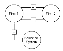
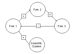
Intra-firm innovational efforts are not considered by both of the two firms in the first simulation (gii = 0). Therefore firm 1 receives innovations only from the scientific system, whereas firm 2 uses the innovative potential of firm 1 for innovating activities (g21 > 0). The exploitation of the innovative potential of firm 1 by firm 2 results in a negative interaction coefficient g12 and thus in a spillover effect having negative impact on firm 1. Fig. 6 shows these interdependencies in a schematic form.

Fig 6
Figure 6. Interdependencies of the agents regarded in the first simulation

3.6
The choice of the signs of the interaction coefficients gij corresponds, regarding the field of innovations, to a predator-prey situation in biology, e.g. in Lotka-Volterra-Systems. Due to the fact that the economic system depends additionally on changes in labour force and capital stock the analogy is rather incomplete. Nevertheless Lotka-Volterra-Systems are used in economics to model business cycles explicitly, e.g. by Gabisch, Lorenz (1987) and Nijkamp, Reggiani (1998).

3.7
At first the behaviour of firms for different values of the interaction coefficient g11sci will be investigated. In other words, the effect of different transfer activities between the scientific system and firm 1 is considered. The initial values for the input factors of both firms used in the simulations are listed in Table 2.

Table 2: Initial values for the simulations with different values of g11sci

Ki(τ = 0)Li(τ = 0)Ii(τ = 0)
Firm 11.00.51.0
Firm 21.00.51.0

.

3.8
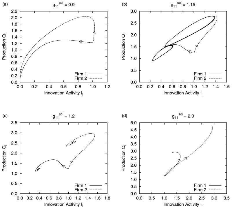
Figures 7 (a) - (d) show the results of the corresponding simulations. Special attention shall be paid to the evolution of the innovation activities Ii and productions Qi. For the first chosen value of the transfer coefficient g11sci = 0.9, the support from the scientific system is rather insufficient. This circumstance and lacking intra-firm research and development (gii = 0) are the reasons why innovation activity Ii cannot be increased by the two firms, see Figure 7(a). Firm 2 can keep its innovation activity approximately constant at the beginning of the simulation and can increase its production, whereas the innovation activity of firm 1 is decreasing immediately from the beginning. This decrease leads to a decrease of the innovation activity of firm 2 later on because its evolution depends solely on the innovation activity of firm 1 since the interaction coefficient g21 is positive and there is no intra-firm research and development (g22 = 0). The productions of both firms evolve with the innovation activities towards zero. This is a rather unrealistic case, because if such a situation occurs in practice the firms would change their investment behaviour or would do research and development of their own to become independent of the scientific system. This case of intra-firm research and development will be investigated later in this article.

3.9
If the support from the scientific system reaches a critical threshold value (g11sci = 1.15) a limit-cycle appears as shown in Figure 7 (b). Both firms are producing with profit, whereby innovation activity Ii and production Qi for each firm increase and decrease cyclically. The period of one cycle is about 200 scaled time units which can be seen from the temporal evolution of the firms that is not shown here. Capital stocks and labour forces show the same oscillation behaviour as the innovation activities and productions. It becomes clear, that the suppression of firm 1 by firm 2 (which is surely not intended by firm 2, because its success depends mainly on the success of firm 1) leads to a collapse of firm 2 itself. This collapse enables firm 1 to recover and the cycle starts again. Remarkable is the further increase in production at high values of innovation activity, although innovation activity is already decreasing. On the other hand production is slightly decreasing when innovation activity is starting to increase again.

3.10
For a larger value of the coefficient describing the support from the scientific system (g11sci = 1.2) the limit cycle vanishes and after few oscillations, the system ends up in a stable equilibrium point with positive innovation activity and production in both firms as shown in Figure 7 (c). Again there is a strong positive correlation between innovation activity and the corresponding production. Nevertheless, at the points were innovation activity starts to decrease, production is increasing further for a short time due to the other production factors capital stock and labour force that are not decreasing immediately with innovation activity.

3.11
With increasing support from the scientific system the stable equilibrium point is shifted towards larger values of production and innovation activity. Choosing the value of the transfer coefficient to g11sci = 2.0 the production in equilibrium becomes twice as large compared to the former case with g11sci = 1.2, whereas innovation activity becomes nearly three times larger, compare Figure 7 (d) with Figure 7 (c). The evolution of both firms from their initial values of innovation activity and production to the stable equilibrium point now takes place without oscillations in a rather straight manner.

3.12
It is worthwhile to emphasise that the positions in phase space and also the characteristics of the equilibrium points are depending on the values of the system parameters. In practice these parameters are changing over time, especially the interaction coefficients between the firms gij and between the firms and the scientific system giksci. So in practice the system will not reach a situation of equilibrium but it will evolve towards equilibrium in time periods in which the parameters are constant.

3.13
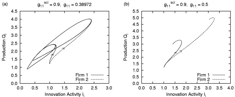
After studying the impact of transfer activities from the scientific system with different strength (different values for g11sci) we want to show now that insufficient support from the scientific system can be compensated with research and development activities within the firms (intra-firm R&D). For demonstrational purpose we take the example of the two-firm-system with a transfer-coefficient g11sci = 0.9. At this strength of the scientific support both firms cannot survive without intra-firm R&D as can be seen in Figure 7 (a). Research and development activities within the firms will be simulated by choosing the coefficient g11 to values greater than zero. This means that firm 1 is doing intra-firm R&D. Firm 2 is assumed to do still no intra-firm R&D (g22 = 0). The simulations are carried out for a period of 1000 scaled time units. The results for innovation activity Ii and production Qi are illustrated in Figure 8.

3.14
As shown in Figure 8 (a) for a value of g11 = 0.38972 a limit-cycle in phase space exists. This limit-cycle only occurs in a narrow range (± 0.00001) around this value of g11. This cycle is separated into two cycles in the subspaces of the two firms shown in Figure 8 (a). These two cycles are overlapping significantly, so firm 1 can improve its market position against firm 2 compared to case of the limit-cycle without intra-firm R&D, shown in Figure 7 (b). The minimal values of innovation activities in the two firms are nearly the same in the two examples with and without intra-firm R&D where a limit-cycle occurs. But the maximal values of innovation activity are much larger in the case of intra-firm R&D: Firm 1 can increase its maximal value of innovation activity by 85% and firm 2 by 65% compared to the limit cycle without intra-firm R&D, Figure 7 (b) and Figure 7 (a). The smaller increase in firm 2 results from the fact that firm 2 still does no own R&D. The spillover effect between the two firms thus is solely responsible for this increase of innovation activity in firm 2.

Fig 7
Figure 7 (a) - (d). Innovation activity Ii and production Qi of both firms for different values of g11sci in the simulation without intra-firm R&D

Fig 8
Figure 8. Innovation activity Ii and production Qi of both firms for g11sci = 1.15 and different values of g11 in the simulation with intra-firm R&D

3.15
In Figure 8 (b) an example with a larger value for the coefficient g11 describing the strength of intra-firm R&D in firm 1 is shown (g11 = 0.5). The limit cycle is not existing here. The stationary point located in phase space at the centre of the limit cycle in the previous example is now a stable equilibrium point, resulting in stationary values for the innovation activities and productions of both firms.

3.16
These stationary values are larger than the corresponding maximal values in the case of the limit-cycle in the previous example (g11 = 0.38972 ), compare Figure 8 (a) and (b). So with increasing importance of R&D activities within firm 1, innovation activity and production is increasing. The stationary values of innovation activity and production are as large as the corresponding values in the example with g11sci = 2.0 and g11 = 0, compare Figure 7 (d) and Figure 8 (b), although the value of g11 = 0.5 in the case of intra-firm R&D does not fully compensate for the difference of the scientific support in the example with g11sci = 0.9, g11 = 0.5 and the example with g11sci = 2.0, g11 = 0.

3.17
To summarise the results of the previous two simulations one can say that intra-firm R&D activities can compensate for insufficient support from the scientific system. Moreover the strength of this intra-firm R&D can be smaller than the strength of the substituted transfer activities from the scientific system to achieve similar quantitative results.

3.18
In the following we will focus on the case g11sci = 1.15 and g11 = 0 in other words we assume that there is no intra-firm R&D and the spillover effects from the scientific system are large enough for the occurrence of a limit-cycle. We will examine the system with respect to different initial values for capital stock Ki, labour force Li and innovation activity Ii. For every initial condition listed in Table 3 the evolution of the system is calculated for a period of 1000 scaled time units.

Table 3: Initial conditions for the simulations with g11sci = 1.15 and g11 = 0

Initial conditionK1(τ = 0)L1(τ = 0)I1(τ = 0)K2(τ = 0)L2(τ = 0)I2(τ = 0)
A3.801.001.305.001.302.50
B4.201.201.004.200.400.80
C0.300.020.350.300.020.35
D0.300.020.200.300.020.20
E1.000.501.001.000.501.00

3.19
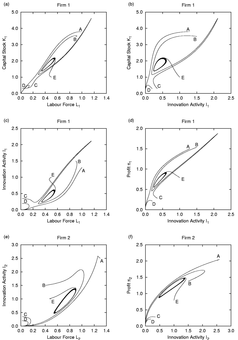
The results are illustrated in Figure 9. Let us first take a look at the relation of the capital stock K1 and labour force L1 for firm 1, Figure 9 (a). For the initial conditions B and C the system ends up in a stable equilibrium point in the upper right corner of Figure 9 (a). When this point is reached, the ratio K1/L1 remains constant. This stability point confirms to the results obtained in neoclassical models, according to which a stable equilibrium point for the ratio K1/L1 is existing (Zhang 1990, Gandolfo 1980). For the initial condition A, capital stock K1 is approximately proportional to L1, so K1/L1 is nearly constant. In case of the limit-cycle the ratio of capital and labour is changing dramatically at the points of turn. Between these points K1/L1 is again approximately constant.

Fig 9
Figure 9 (a) - (f). Simulation of the dynamics of two firms with different initial conditions and g11sci = 1.15 without intra-firm R&D

3.20
Initial condition A shows that large values of capital stock, labour force and innovation activity does not guarantee a prosper evolution of both firms. The suppression of firm 1 by firm 2 due to the spillover effect between the two firms having negative impact on firm 1 of leads to a collapse of both firms.

3.21
Under initial condition B firm 1 is first evolving in direction of bankruptcy (Figure 9 (a) - (d)). Firm 2 is causing this development again due to the spillover effect having negative impact on firm 1. This development continues until the profit of firm 2 has declined to values below that of firm 1. Firm 1 can evolve then without considerable negative impact from firm 2 and its profit reaches the stable equilibrium point.

3.22
For the initial conditions C and D it is demonstrated, how a small difference in the initial conditions for R&D can affect the whole evolution of the firms. As shown in Figure 9 (d) this difference decide in case of firm 1 about surviving on the market. Under initial condition C, firm 1 increases its capital stock K1 and labour force L1 at first, whereas its innovation activity decreases slightly as one can see in Figure 9 (b) and (c). At larger values of K1 and L1 innovation activity starts to increase and the system ends up in the same stable equilibrium point as for initial condition B.

3.23
For initial condition E the system ends up in the stable limit cycle, see also Figure 7 (b). The profit (i of both firms is oscillating between the two extrema and depends highly on their innovation activities as shown in Figure 9 (d) and (f). In this case profit of firm 2 reaches higher levels than profit of firm 1, as is also valid for capital stock, labour force and innovation activity.

3.24
From the shape of the trajectories, shown in Figure 9, one can conclude, that for the set of parameters used in this simulation, a stable equilibrium point in the upper right corner of Figure 9 (a) - (d) exists, as well as a stable limit-cycle and a saddle point, which lies in the lower left corner of Figure 9 (a) - (d). The saddle point is a critical unstable point which decides upon the success of firm 1 on the market.

Simulation of innovation diffusion processes

3.25
We will now study the dynamic behaviour of three decision making firms that have different co-operation strategies. Here decision making stands for changing the ratios of investment over time. As mentioned in section 2.2decisions concerning marketing or co-operation strategies are not considered in this article. As in the previous simulations firm 1 is the only one which receives know-do transfers from the scientific system. The interaction coefficients gij describing the impacts of spillover effects between the firms are chosen as schematically depicted in Figure 10: Firm 2 benefits from innovations of firm 1 (g21 > 0). Contrary to the previous simulations there will be no negative feedback to firm 1 from firm 2 (g12 = 0). Such a constellation is realised in practice for example by a licence agreement between firm 1 and firm 2. So the disadvantages for firm 1 that are arising from firm 2 by also bringing the innovation to market are at least partially compensated with payments to firm 1. Firm 3 benefits of innovations in firm 2 (g32 > 0). We assume that there will be no negative feedback on firm 2 from firm 3 as well (g23 = 0). But it is assumed that firm 3 is in a competing situation to firm 1 (g13 > 0). This is an example of a constellation for which it is possible that innovation diffuse in the whole system.

3.26
In order to investigate what happens to an innovation impulse in this system the know-do D1sci of the scientific institution will be artificially increased from its initial value D1sci = 1.0 to D1sci = 1.4 for a period of 50 scaled time units at a time of τ = 1000 after the whole system has reached equilibrium. The values of the system parameters are listed in Table 4. As already noted in section 2 the parameters f (nm) are set equal to 1.0. The initial values of the simulations are listed in Table 5.

Fig 10
Figure 10. Interdependencies of the agents regarded in the simulation of innovation diffusion


Table 4: Parameters in the simulation of innovation diffusion

Global parameters

abα1α2rD1sciIr

1.01.00.50.50.1[1.0 ; 1.4]1.0
Firm specific parameters
Yimaxsiwiδiνiγi
Firm 16.00.60.40.11.00.1
Firm 26.00.60.40.11.00.1
Firm 36.00.60.40.11.00.1
gi1gi2gi3gi1sciεiεi
Firm 10.000.00-0.401.150.11.0
Firm 20.210.000.000.00.11.0
Firm 30.000.210.000.00.11.0


Table 5: Initial values for the simulation of innovation diffusion

Ki(τ=0)Li(τ=0)Ii(τ=0)µiK(τ=0)µiL(τ=0)µiI(τ=0)
Firm 13.50.71.20.30.20.5
Firm 23.50.71.20.30.20.5
Firm 33.50.71.20.30.20.5

3.27
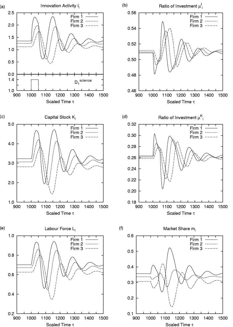
In Figure 11 the results of the simulation are depicted for the interesting time period from 900 to 1500 scaled time units. The market share mi of firm i is calculated according to:

Eqn 18 (18)

whereby the assumption is included that all firms belong to the same industrial sector.
3.28
At a time of τ = 1000 the system, that has reached its equilibrium state, is artificially distorted by the innovation impulse in the scientific system. This impulse leads to a large increase of innovation activity in firm 1, followed by firm 2 and firm 3 as illustrated in Figure 11 (a).

3.29
Maxima and minima of the capital stock Ki and the labour force Li in each firm are slightly delayed compared to the corresponding innovation activity Ii, compare Figure 11 (a), (c) and (e). The increase in innovation activity is causing an increase in production and therefore an increase in capital stock and labour force due to increasing investments.

3.30
A noticeable time-delay occurs between the maxima of innovation activity in the three firms as one can see in Figure 11 (a). This phenomena can be interpreted as a process of innovation diffusion. Firm 1 is the first that benefits from the know-do impulse in the scientific institution. Firm 2 follows with a delay in time, because it has to collect enough know-do concerning the new innovation, before it can implement the innovation. The maxima of innovation activity of the three firms are separated by about 20 scaled time units. The delays in the diffusion process of innovations are often mentioned in the corresponding literature, see for example Freeman (1988), Maier (1998) or Silverberg (1991). They are caused by insufficiencies in the process of information collecting and implementing the knowledge gained this way to new products.

3.31
The innovation impulse reaches firm 3 with a considerable delay, because firm 3 is not benefiting directly from firm 1. The maxima of innovation activity in firm 2 and firm 3 reach not as large values as in firm 1. The reason for this is that innovation activity in firm 1 is already declining when the maxima in firm 2 and firm 3 are reached. The decline in innovation activity of firm 1 is caused by firm 3 due to its negative network effect on firm 1 (g13 < 0), besides the increasing importance of the term -γ Ii in (11) with larger values of the innovation activity Ii.

Fig 11
Figure 11. Time evaluation of three firms in the simulation of innovation diffusion

3.32
After the innovation impulse from the scientific institution has finished further innovation cycles start that are not caused directly by impulses from the scientific system. The cycles have periods of 100 to 120 scaled time units. To compare the time scales of the simulations with practise we want to give an example of chip production in computer industry. The product life-cycle of computer chips is between 12 to 24 month (Maier 1998). So if one identifies the innovation cycles with the observed cycles in chip design, 100 time units in the simulation correspond to somewhat between one and two years in practice.

3.33
The maximum values of innovation activity in the second cycle that occurs between the scaled time 1100 and 1250 reach as large values as the corresponding maxima in the first cycle that is caused by the scientific system. In the third and forth cycles the maximum values of innovation activity in the firms are much smaller.

3.34
From the strategic behaviour of investment of firms, depicted in Figure 11 (b) and (d), it becomes obvious that a change in the ratios of investment effects the development of the corresponding variable (capital stock K, labour force L and innovation activity I) several time steps later. The firms can not adjust their behaviour of investment instantly to a new economic situation. The ratios of investment in labour force µiL, which are not shown here, are behaving similarly to the ratio of investment in innovation activity µiI, depicted in Figure 11 (b). Both together evolve anti-cyclically to the ratios of investment going into capital formation µiK, shown in Figure 11(d).

3.35
An analysis of market shares show that the market share of firm 2 is evolving much smoother than the market shares of the other two firms. Firm 1 is able to increase its market share at the beginning of the innovation impulse from the scientific institution at the expense of the other two firms. Firm 1 rules the market at this time because it was the first firm that introduced a new innovation on the market. Firm 2 and firm 3 can increase their market shares when the innovation activity of firm 1 has declined significantly. Firm 3 gains a considerable market share several time periods later and becomes market leader at the end of the first innovation cycle, after it has also established the innovation. At this point in time innovation activity and market share of firm 1 has reached its minimum.

3.36
The gain in market share of firm 2, which adopts the innovation early compared to firm 3, is not as large as that of firm 3. A similar observation was made by Silverberg (1991). He found that very early adopters experience market share and profitability losses, whereas adopters that make use of the innovation later, but not too late can take more advantage of it. The market situation for firm 2 is little better during the second innovation cycle. At the beginning it loses again market share but can recover, whereas the market share of firm 3 is collapsing dramatically during this innovation cycle. This time, firm 3 is adopting the innovation too late. The problem of optimal timing the adoption of innovations is also mentioned by Maier (1998).

3.37
The accumulated production of the three firms, not illustrated here, shows a cyclical development with maxima of production in times of high overall innovation activities of all firms and minima of production in times of low overall innovation activities. This behaviour is reasonable, since if new innovations enter the market, the market-potential as a whole can be increased due to increasing demand for the new or improved products. On the other hand the demand becomes saturated over time, if no new innovation follows.

* Concluding remarks

4.1
The development of inter-linked firms belonging to different sectors and the existence of stable points of equilibrium depend mainly on the impact of spillover effects between the different firms on the market and the impact of the scientific system. For special constellations the occurrence of a stable limit-cycle can be observed. In such a situation the firms are permanently fighting for the leading market position.

4.2
In numerical simulations of two firms we show that insufficient support from the scientific system can be compensated by research and development activities within the firms. Moreover the strength of this intra-firm R&D can be less than the strength of the transfers activity from the scientific system that is substituted by intra-firm R&D to achieve similar quantitative results with regard to innovation activity and production.

4.3
One further important result from the simulations of two firms above show the fact that large increases in innovation activities (innovation pushes) can be caused by spillover effects, without the existence of random events. So besides random events which play an important role in the context of the development of new products, an increase in innovation success can be made by the concentration of the labour forces and the knowledge base (know-do) of several firms and the scientific system.

4.4
Diffusion of innovation caused by transfer activities from the scientific system and spillover effects between firms is observed in the simulation of three firms. These diffusion processes come along with time-delay effects that are caused by inefficiencies in collecting information and implementing the new knowledge gained this way in new products.

4.5
The simulations above confirm the result of Silverberg and Maier, that the timing of adopting an innovation from other firms has much impact on the development of future market shares. If innovations are adopted to early or to late, less market share can be gained compared to the case when the adoption takes place at the optimal time, determined by the current stock of knowledge.

4.6
We focused our point of view mainly on the supply side of the market. Modelling also the demand side endogenously would provide for a more realistic and comprehensive description of the economic system. But the price to be paid would be very high with respect to the modelling complexity. However, in order to get a detailed insight into the complex inter-linked activities of firms behaving under profit maximisation conditions, it seems to be justified even to continue in studying further selected examples of specific economic networks of firms. Especially the role of know-do supporting institutions has to be further investigated. Of course, the described modelling framework has its shortcomings. But with respect to the insights into the complex decision processes of co-operating and competing firms, which can be gained, a further research in this direction is needed.


* Notes

1 The Cobb-Douglas production function is only used for illustrative purpose.


* References

ANDERSSON, A. E. (1981): Structural Change and Technological Development. Regional Science and Urban Economics 11, 351-361.

ANDERSSON, A. E., MATSINEN, J. (1980): Mobility of Resources, Accessibility of Knowledge and Economic Growth. Behavioural Science 25, 353-366.

ARROW, K. J. (1962): The economic implications of learning by doing. Review of Economic Studies 29, 155-173.

ARTHUR, W. B. (1989): Competing Technologies, Increasing Returns, and Lock-In by Historical Events. Economic Journal 99, 116-131.

AUDRETSCH, D. B. (1996), Industrieökonomik. In: Von Hagen, J., Börsch-Supan, A., Welfens, P. (eds.): Handbuch der Volkswirtschaftslehre I. Springer, Berlin Heidelberg New York, pp. 178-218.

CANTNER, U., PYKA, A. (1998): Technological Evolution - An Analysis within the Knowledge-based Approach. Structural Change and Economic Dynamics 9, 85-107.

Cigno, A. (1981): Growth with Exhaustible Resources and Endogenous Population. Review of Economic Studies 48, pp. 281-287.

FISCHER, M. M., MENSCHIK, G.(1994): Innovationsaktivitäten in der östereichischen Industrie: Eine emprische Untersuchung des betrieblichen Innovationsverhaltens in ausgewählten Branchen und Raumtypen. Abhandlungen zur Geographie und Regionalforschung, Band 3. Institut für Geographie der Universität Wien.

FREEMAN, C. (1988): Diffusion: The Spread of New Technology of Firms, Sectors and Nations. In: Heertje, A (ed.), Innovation technology, and Finance. The European Investment Bank. Basil Blackwell, Oxford.

GABISCH G, LORENZ, H. W. (1987): Business Cycle Theory. Lecture Notes in Economics and Mathematical Systems. Vol. 283. Springer, Berlin Heidelberg New York.

GANDOLFO, G. (1980): Economic Dynamics: Methods and Models. Advanced Textbooks in Economics. North Holland publication company, Amsterdam.

HAAG, G. (1989): Dynamic decision theory: Applications to Urban and Regional Topics. Studies in Operational Regional Science. Kluwer Academic Publishers, Dordrecht.

HIPPEL, E. VON (1988): The Sources of Innovation. Oxford University Press, New York.

HIPPEL, E. VON (1989): Cooperation Between Rivals: Informal Know-how Trading. In: Carlsson, B. (ed.): Industrial Dynamics. Kluwer Academic Publishers, Boston, pp. 157-175.

JUNGMITTAG, A., BLIND, K., GRUPP, H. (1999): Innovation, Standardisation and the Long-term Production Function. Zeitschrift für Wirtschafts- u. Sozialwissenschaften 119, 205-222, Duncker & Humblot, Berlin.

KOBAYASHI, K., SUNAO, S., YOSHIKAWA, K. (1993): Spatial Equilibria of Knowledge Production with 'Meeting-Facilities'. In: Andersson (ed.). The Cosmo-Creative Society. Logistical Networks in a Dynamic Economy. Springer Berlin Heidelberg New York, pp. 237-259.

LUCAS, R. (1988): On the Mechanics of Economic Development. Journal of Monetary Economics 22, 3-42.

MAIER, F. H. (1998): New product diffusion models in innovation management - a system dynamics perspective. System Dynamics Review 14 (4), 285-308.

MÜLLER, K. H., HAAG, G. (1996): The Austrian Innovation System, Complex Modelling with NIS-Data. Final report Vol. 5. Institute for Advanced Studies, Vienna.

NELSON, R. R., WINTER, S. G. (1982): An Evolutionary Theory of Economic Change. Belknap Press of Harvard University Press.

NIJKAMP, P., REGGIANI, A. (1998): The Economics of Complex Spatial Systems. Elsevier, Amsterdam.

OECD/EUROSTAT (1997): Oslo Manual: Proposed Guidelines for Collecting and Interpreting Technological Innovation Data.

PYKA, A. (1999): Der kollektive Innovationsprozeß. Volkswirtschaftliche Schriften Heft 498. Duncker & Humblot, Berlin.

ROMER, P. M. (1986): Increasing Returns and Long-run Growth. Journal of Political Economy 94, 1002-1037.

ROMER, P. M. (1990): Endogenous Technological Change. Journal of Political Economy 98, 71-102.

SCHUMPETER, J. A. (1934): Theorie der wirtschaftlichen Entwicklung. 9th edition 1997. Duncker & Humblot, Berlin.

SILVERBERG, G. (1991): Dynamic Vintage Models with Neo-Keynesian Features. In: Technology and Productivity: The Challenge for Economic Policy. The Technology Economy Programme. OECD, pp. 493-507.

SILVERBERG, G. (1997): Is there Evolution after Economics? In Schweitzer, F. (ed.): Self Organization of Complex Structures, From Individual to Collective Dynamics. Gordon and Breach Science Publishers, Amsterdam, pp. 415-425.

SILVERBERG, G., LEHNERT, D. (1994): Growth Fluctuations in an Evolutionary Model of Creative Destruction. In: Silverberg, G. Soete, L. (eds): The Economics of Growth and Technical Change. Edward Elgar Publishing, Aldershot, pp. 74-108.

SOLOW, R. (1956): A Contribution to the Theory of Growth. Quarterly Journal of Economics 70, 65-94.

TEECE, D. J. (1998): Capturing Value from Knowledge Assets: The New Economy, Markets for Know-How, and Intangible Assets. California Management Review 40, 55-79.

WEIDLICH, W, HAAG, G. (1983): Concepts and models of a quantitative sociology. Springer Berlin Heidelberg New York.

WITT, U. (1995): Moralität vs. Rationalität - Über die Rolle von Innovation und Imitation in einem alten Dilemma. In: Wagner, A., Lorenz, H. W. (eds.): Studien zur Evolutorischen Ökonomik III. Schriften des Vereins für Sozialpolotik. Band 195/III. Duncker & Humblot, Berlin, pp. 11-33.

WOECKENER, B. (1993): Innovation, Externalities and the State, a Synergetic Approach, Journal of Evolutionary Economics 3(3), pp. 225 -248.

WOECKENER, B. (1995): Hotelling-Modelle der Konkurrenz und Diffusion von Netzeffektegütern, deterministische und stochastische Ansätze zur Erklärung der Ausbreitung neuer Kommunikations- und Gebrauchgüter-Systeme. Francke-Verlag, Tübingen Basel.

ZHANG, W.B. (1990): Economic Dynamics: Growth and Development. Lecture Notes in Economics and Mathematical Systems. Springer, Berlin Heidelberg New York.

ZHANG, W.B. (1999): Capital and Knowledge: Dynamics of Economic Structures with Non-Constant Returns. Springer, Berlin Heidelberg New York.

----

ButtonReturn to Contents of this issue

© Copyright Journal of Artificial Societies and Social Simulation, 2001