This paper presents a new approach to infectious disease analysis through computer simulation. The case study concerns the spread of Bovine Leukemia, a viral pathology sustained by a retrovirus from the same family as HIV that exclusively strikes cattle within dairy farms. Although analytical models of epidemic spread have been implemented, their practical use is often difficult, above all for predictive and quantitative analysis. Computer simulation provides a new possible approach, and here we apply two methodologies: "System Dynamics" and "Agent Based". Furthermore the case study is used like a workbench to illustrate the differences between the two approaches and to explain how these techniques can help with the understanding of the problem. At the same time epidemiological researchers are able to do a preliminary "what-if" analysis with the purpose of assessing the system's behaviour under various conditions and evaluating which alternative sanitary policies to adopt. Thanks to model results, experts have reached their first suppositions in order to fight the endemic behaviour of Bovine Leukemia. The models implemented can easily be extended to collect the details of the system to be investigated more efficiently and to allow more refined analyses to be made.

Keywords:

Agent-based Modelling; Epidemics; System Dynamics

Introduction

1.1

In recent years news reports have highlighted the problem of epidemics on animal farms. Two episodes have particularly struck the European public opinion: BSE and foot-and-mouth disease. The first one mainly for the tragic consequences that it has had on man.

1.2

Even if humans are not directly in danger, since the infective agent is not considered able to "jump species", economic damage is however, considerable, represented by loss of animals, the negative effects on meat markets, by resources required to implement control and eradication policies.

1.3

One of these epidemics is Bovine Leukemia, a viral pathology, sustained by a retrovirus from the same family as HIV that exclusively strikes cattle, weakening the infected animals and causing downturns in milk production. Despite a national plan for eradication adopted some years ago, with the obligatory elimination of infected animals, disease cases of endemic character are still recorded.

1.4

In cases like this, the construction of a model that represents the epidemic dynamic can constitute a valid tool in decisional and control processes for the people responsible for intervention policies. More specifically, it supports the identification of factors and mechanisms of epidemic spread exactly during the descriptive phase and it allows the sifting of different scenarios in a reasonably rapid way. This characteristic is essential in order to be able to carry out a qualitative and quantitative evaluation of defence strategy choices and of their consequences in order to select the best combination of control and eradication techniques.

1.5

From a historical perspective, the development of epidemic models has passed through two main phases; initially, during the first decades of the XXth century, researchers elaborated analytical models where the system was formally described by systems of time dependent differential equations. One of the major difficulties with this approach has been the rapid growth of the mathematical complexity of the systems used to describe the various aspects of phenomena in sufficient detail and the difficulty in solving them in an analytical form. Hence, their practical use in specific cases is very limited.

1.6

A second phase is represented by the current trend in the development of models in epidemiology which date back to an increasingly wider use of computers. Initially they were utilised merely to estimate parameters that maximized the overall likelihood of simple models carrying out optimisation programs. Nowadays the aim is to build entire simulation models that permit a more practical approach and where results are obtained even for highly complex problems.

1.7

In this article, we describe two computer simulation models in detail, respectively established on System Dynamics and Agent based techniques that we have developed to analyse an epidemic of Bovine Leukemia on a typical dairy farm. We also underline the differences between these new approaches and the more traditional mathematical treatment of infectious diseases.

1.8

The remainder of this paper is organized as follows: Section 2 presents a brief survey of the traditional biomathematic approaches that can be found in scientific literature used to construct an epidemic model; Section 3 sketches the main guidelines used to develop our computer models; Section 4 explains the case study i.e. the principal Bovine Leukemia characteristics, essential to the understanding of the design of our model; Section 5 briefly analyses the structure of the models and their leading features; Section 6 and 7 concern model calibration and practical experiments implemented so far while their first outcomes, as well as practical and theoretical conclusions of this experience, are discussed in the last section.

Biomathematical models of epidemics: a survey

2.1

The remarkable impact upon economics in the case of animal diseases, and on public health in human infections, have given impulse to the development of representative models of epidemic evolution and propagation (Bailey 1975; Renshaw 1991; Hoppensteadt 1975; Bartlett 1960). The most important, from a historical point of view, and for the number of applications and developed analysis are time dependent differential equation systems (deterministic models SIR, SI, etc.) and differential equations systems of time dependent distribution probability functions (probabilistic models).

Deterministic model SIR and its by-products

2.2

The SIR model is the point of reference for mathematical models used to describe epidemic spread. A first version was elaborated by W.O. Kermack and A.G. McKendrick in 1927. Most current epidemiological models are extensions of it.

2.3

The model divides population into three fundamental blocks:

s (susceptible)

that is subjects susceptible to contracting the infection;

i (infected)

the subjects that have already contracted the infection, to the stage of full development or incubation, so they are vectors of contagion;

r (retired)

subjects that have died or that have developed immunity to the contagion, therefore no longer able to infect or to contract infection.

2.4

Three differential equations describe time evolution of population P components. We suppose P constant to simplify.

where the meanings of parameters are:

β

(infection-rate or contact-rate) rate of new infected in the unit of time;

γ

(removal-rate) rate of mortality or immunity in the unit of time.

2.5

Therefore we are able to foresee the temporal trend of infection estimating β and γ parameters, and knowing the initial values (s₀, i₀, 0) at time t₀. In practice we are more interested in the derivative of r, that is the "epidemic curve", given by the new retired rate. The importance of this curve is due to the format normally available for epidemiological data: the number of new deceased / recoveries in the last unit of time (generally day or week).

2.6

The epidemic curve, solution of the above equations, has been found in approximate form (Kermack and McKendrick, 1927), and in parametric form (Kendall 1956).

2.7

The famous Kermack and McKendrick "Threshold Theorem" has derived from these equations: naming ρ = γ/β the relative removal-rate, no epidemic can spread unless we had the initial condition s₀ > ρ. Defining ν = s₀ - ρ and under some approximations, the "total size of epidemic", that is the total number of subjects infected, for t → ∞ is 2ν. In other words:

2.8

In the case of non deadly or non symptomatic disease it is possible to use a simplified model called SI. It does not keep track of retired ones and solutions are simpler and more immediate.

2.9

Over the years, the model presented has been extended by the same authors and by other researchers to consider other arguments such as: the presence of carriers (apparently healthy individuals who harbour infection), the spread of illnesses through vectors (bugs, water, food, etc.), several groups of subjects coexisting (with different rates of infectivity, mortality and immunity), other states apart from infected and susceptible (for example, immunity from a previous exposure to contagion), the contemporary action of several viral agents, incubation periods and so on.

2.10

Although the deterministic model is the basis of the biomathematical approach, it is not valid for small populations, in which events are subject to ample statistic fluctuations, and for non homogeneous populations with different degrees of immunity, density, exposure to contagion factors, etc. So researchers have developed more complex models.

Stochastic model

2.11

As with its deterministic counterpart, the epidemic stochastic model divides population into three blocks which can be described using random variables s(t), i(t)and r(t), that represent respectively the number of susceptible, infected and retired subjects at time t (with s(t) + i(t) + r(t)= n + a where n is the initial number of susceptibles and retired and a is the number initially infected). In an analogy with a deterministic model we always define infection and removal rates:

2.12

Using the relative removal rate ρ = γ/β and the scaled time τ =tβ, the probability p_si(τ) that at time τ there are exactly s susceptible subjects still uninfected and i infective subjects in circulation is determined by differential-difference equation:

2.13

Solutions have been found over the years, particularly using recursive techniques (Billard 1973). However, as with the case of the deterministic model, the main problem is how to apply formulas to the real world.

Other models

2.14

Other models have been developed that keep track of the geographical distribution of population components (S,I,R), besides the temporal one: these are spatial models. In other words the above differential equations describing the spread of infectious disease are not only dependent on time but also on two-dimensional coordinates (x, y). So that we analyse the gradients of the functions s(x, y, t), i(x, y, t), r(x, y, t).

2.15

Another important class of models no longer consider processes that occur in continuous time but assume that, following the contraction of infection by any susceptible subjects, there ensues a latent period of fixed length. The subsequent infectious period is considered as being contracted to a single point of time. These are the so called discrete-time or chain-binomial models (Gani 1969; Gani and Jerwood 1971).

2.16

If we indicate p=1-q as the chance of adequate contact, sufficient for the transmission of the infection from an infected subject to a susceptible one, and:

I_t:

is the random variable indicating the number of the infected just prior to time t which become infectious at time t;

S_t:

is the usual random variable indicating the susceptible remaining uninfected at time t;

we have:

S_t = I_t+1 + S_t+1

2.17

If we also suppose that a susceptible subject's chance of being infected depends only on the presence of some infective subjects and not on their actual number, we obtain the Greenwood model:

This can be rewritten in a form that depends only on the susceptible variable, so that we obtain a univariate Markov chain expression:

2.18

If we assume instead, that the chance of infection does depend on the number of infectives present we obtain the Reed-Frost version.

Computer simulation

3.1

Notwithstanding important results reached in the qualitative and quantitative description of the evolution of infectious diseases, the analytical approach suffers from intrinsic limits. First of all the differential equations that represent real situations often have no analytical solution so that related specific models are based on assumptions and simplifications. For small populations, in which events are subject to ample statistic fluctuations, only the stochastic model remains valid, but it is more difficult to manage and to solve.

3.2

For non homogeneous populations, as in our case study, the equation number "explodes" if every sub-population and corresponding infection rates (within and between groups) and removal rates are considered. In many cases, it is difficult, or even impossible, to find the analytical form of the equations (consider, for instance, the retirement process of our case study, where infected animals are simultaneously butchered when they are detected as positive at sanitary controls which happens at variable intervals).

3.3

As illustrated above, the application of an analytical approach to the real world is often difficult, especially for practical use in predictive and quantitative analysis.

3.4

To overcome these hurdles Monte Carlo techniques have been already used (Elveback et al. 1971; Elveback 1971; Ewy et al. 1972; Gallop 1999) to challenge the complexity of stochastic models and Markov chain models.

3.5

We have developed another approach through computer simulation which is not confined to the Monte Carlo technique. This is an alternative to methods used so far to define epidemic descriptive / predictive models. "System Dynamics" and "Agent Based" paradigms have been chosen from the vast number of models and simulation techniques available (Law and Kelton 2000; Banks 1998; Gilbert and Troitzsch 1999).

3.6

The first method is a more traditional one, while we focus on time dependent systems of difference equations and their iterative solutions (Forrester¬Ý 1961). This technique descends directly from the time dependent systems of integro-differential equations used to describe dynamic systems. We can use various function forms, even non-analytical ones, this way we have the advantage of reproducing actions whose execution may depend upon external conditions (like controls issues). The main characteristics of System Dynamics are that the domains of variables are continuous and all dependent on the time parameter; furthermore they are connected by feedback, so that the variable x_i at time t+1 depends on variable x_j at time t, t-1,...,0. Moreover the interdependencies between the variables of the system are highlighted thanks to a standardized graphically descriptive language: the so called structural diagram.

3.7

With system dynamics classical techniques, the population characteristics are aggregate variables and the model describes the change of these variables as a whole system, as in Hemorrhaging Dengue Fever study (Ritchie-Dunham 1995a; Ritchie-Dunham 1995b). We have used the commercial product "Vensim" to implement our model.

3.8

The "Agent Based" archetype, on the other hand, models the real world domains as a set of behaviours of agents. It is not necessary to explicitly model the interactions of the different factors since, conforming to the characteristics of the agent-based modelling, the overall dynamics of the infection is the result of the different events that interest the single agents. So we have an "interaction-oriented" modelling paradigm. Agent Based modelling is particularly useful in the study of complex systems that exhibit non linear behaviour, like ecosystems and financial markets.

3.9

To implement the model described here we have used the Swarm environment. Further information on this project is available in (Johnson and Lancaster 2000; Luna and Stefansson 2000; Swarm Dev. Group 2000). The way both models have been applied to the case study will be explained in detail in the following paragraphs.

The case study

4.1

Enzootic Bovine Leukemia is a viral pathology sustained by a retrovirus from the same family as HIV that exclusively strikes cattle. Leukemia is not fatal for most infected animals, but a small percentage of them develop a malignant form. The infected animals remain serum-positives for life, so they are exposed to secondary infections, due to the weakening character of the illness, and consequently become less productive. Moreover, serum-positive cattle are ineligible for export to many countries.

4.2

In order to avoid a great increase in the spread of the infection among farms and to improve the efficacy of legislation prohibiting the sale of infected animals, rapid identification and elimination^[1] is essential. Hence since 1996 an obligatory national plan for eradication following sanitary controls at frequent intervals has been set up in Italy. The frequency of the controls depends on the identification of cases of infection. The adoption of this plan has certainly contributed towards the limitation of the spread of the infection, but, to date, disease cases of endemic character are still being recorded, especially in farms situated in Central and Southern Italy.

4.3

Hence, a deeper analyses of the matter is required, possibly using new approaches, in order to understand the causes of endemicity of Leukemia, and to appraise the effectiveness of other control measures as alternatives to current ones. To satisfy the need for information and, at the same time, attack an epidemic problem by using different techniques of simulation to compare their results, we began to collaborate with the 'Istituto Zooprofilattico Sperimentale delle Regioni Lazio e Toscana'.

4.4

As will be outlined in section 5, we have adopted the Unified Modelling Language^[2] (UML) formalism (Booch 1999) from the early stages of the project; so that we give a UML pictorial representation of structures in the following paragraph.

Epidemiological issues

4.5

A good understanding of the infection mechanisms and their correct modelling is a fundamental step towards successfully preparing and evaluating alternative strategies that aim to eradicate the disease. In the case of Bovine Leukemia, the scenario is quite complex because there are a series of particular aspects that affect the overall dynamic of contagion.

4.6

First of all, the disease occurs over a long period of time and rarely induces evident clinical symptoms, at least in a short-medium period. Therefore the chances of eliminating an infected bovine (retirement or death) from the farm due to appearance of symptoms are practically negligible. Moreover, an infected animal cannot regain its health, neither can it develop a kind of immunity. As will be made clear later, animals that result infected at periodical controls are butchered , so the application of a mathematical reference with only two groups (susceptible and infected subjects) that do not consider the "retired" appears impossible, but it is not easy to represent this process in a tractable equation.

4.7

Other aspects of epidemiological interest are the period of latency, during which the animal is already infected but cannot transmit the disease to other animals, and a period of serum-conversion, in which the infected (and infectious) animal is not detectable at tests. In our models, we assumed a period of latency of about two weeks, while about other 17 days are necessary to complete the serum-conversion process. It is important to note that this aspect has considerable impact on the simulation structure, especially for the control activities, where it is necessary to distinguish between infected animals that are detectable and those that are not.

4.8

The situation is even more complex for young calves, in which the simultaneous action of infective factors (blood and colostrum) and antibodies eventually assumed through milk can increase resistance to the disease for a period of around six months. All this can be represented in the model with a degree of immunization^[3] which is diversified between adults and young bovines, although at this first stage of simulation we assume a single degree of immunity in order to simplify the model.

4.9

A further difficulty arising in the building of a simulation model of a Bovine Leukemia epidemic is the multiplicity of infective factors, and the limited availability of experimental documentation. Theoretical models of virus transmission include both horizontal and vertical means. In the first category direct contact between animals of the same department are included as well as iatrogenic inoculation by rectal palpation sleeves and the multiple use of surgical instruments used in carrying out vaccinations and artificial insemination. All these means of transmission are accounted for within sector infection rates.

4.10

The vertical means of contagion are represented by transplacental transmission at the moment of parturition and by the administration of milk from infected bovines to young calves during their first days of life, these are the inter-sector infection rates.

4.11

All that concerns the contagion process can be organized in a state diagram that visualizes the various conditions that a bovine can encounter with regard to the disease.

Figure 1. The contagion process

The sanitary controls

4.12

The Italian control policy for bovine leukemia consists of periodic tests conducted on the animals by the Veterinary Services, in correspondence with the national plan for the eradication of the disease. These controls consistently limit the spread of the disease due to the massive elimination of the infected calves at predetermined intervals. Hence, it is a key factor of the control policy and small changes in its organization can determine a completely different behaviour of the epidemic.

4.13

At the moment controls are limited to cows over twelve months old. A specific objective of experts in this subject is to analyse the impact of this choice on the spread of Bovine Leukemia and eventually to elaborate alternative strategies.

4.14

The frequency of controls depends on the results of previous controls. The farms that do not exhibit cases of leukemia acquire a sanitary warranty in order to be able to sell animals. On the other hand, the presence of infected animals determines the carrying out of controls at closer intervals. The farms get the sanitary certification again after two negative consecutive controls, the second of which is performed after a period of quarantine. The situation is well schematised by the UML diagram constructed on the information provided by experts.

Figure 2. The current control policy

4.15

It is necessary to specify that in the case of positive controls the farm must eliminate all the infected cows within one month. According to empirical evidence and to simplify the structure of the simulation, we assumed that all the infected animals are butchered at the end of the period allowed for this operation and hence the latter test is carried out two months after the former.

The organization of a typical farm

4.16

From the evidence reported by experts it is clear that the course of an epidemic of Bovine Leukemia depends on the interaction between the cows and the logistic aspects of the farm.

4.17

The operative ways dairy cows are managed on the farms are strictly related to their physical conditions, in particular to their ability to yield milk and to their possible pregnant state. These aspects reflect the organisation of the dairy farm that is structured in several sectors which are physically separated, each containing a homogeneous group of animals.

4.18

In our simulation models, we have considered a typical medium - large farm from the centre of Italy with a population of a few thousand cows and seven physical sectors which bovines pass through depending on specific events like birth, growth, pregnancy, delivery, nursing, etc. During their lives, usually about five and a half years, the cows go into calf areas immediately after their birth and subsequently they complete the production cycle (insemination, pregnancy, delivery and nursing) three times on average. The life cycle of the bovines is well illustrated by the following state diagram, where even the typical mean times of every state are reported (and hence the typical periods of permanence in the various sectors of the farm).

Figure 3. The typical life cycle of a cow

4.19

It is important to remark that the overall number of cows tends to be in equilibrium with regard to the firm's target because the number of parturitions normally covers slaughterings and the eventual excess can be drained by sales of calves. Anyway the analysis is about a dairy farm so all the males are sold within about eleven days from birth.

Structure of the simulations

The conceptual model

5.1

One of the key factors in constructing a good simulation model is the establishment of close interaction between model makers and subject-matter experts, especially during the early stages of the project, in order to acquire a complete understanding of the system to be simulated and to make a precise formulation of the problem. The result of this activity is referred to as a 'conceptual model' and collects all the information which is considered important (for example, assumptions, algorithms, data summaries) at various levels of detail and by formalisms that can vary from simple lists to complex graphical diagrams.

5.2

In our case, the main sources of information were interviews with the subject-matter experts, evidence taken from scientific literature concerning estimates of the infectivity ratios of the various ways of transmission and a first series of real data acquired from a medium-large Italian dairy farm.

5.3

In this phase we decided to adopt the Unified Modelling Language to document the conceptual model in a formal, but easily comprehensible way and to improve the interaction with experts during the process of representation of the various aspects of the system under study.

5.4

The results of this phase of analysis were a series of 'state diagrams' concerning the life cycle of the animals - consisting in various states that have a close correspondence with the logistics sectors of the farm - the different sources of transmission and the succession of sanitary controls on the farm.

5.5

The definition of states and transitions, although essential for the Agent Based approach, was also very useful for the development of System Dynamics one, allowing an easy and coherent definition in terms of stock variables and dynamic flows. Moreover, state diagrams proved to be an excellent tool to conduct walk-through analyses of the conceptual model to verify its validity.

5.6

The fundamental characteristics of the model and the associated state diagrams have already been described in previous chapter; here we resume and list the principal ones that are common to both implementations.

1. We have three stock variables: susceptible, infected and detectable subjects, and transitions between the three stocks are adjusted according to the SI contagion model basis idea.
2. The "observable set" i.e. variables that are measurable is made up of susceptibles and detectables. The infected is a variable that is fundamental, influences other variables and obviously affects the model behavior. However, the observer will never know its value.
3. The life cycle of dairy cows passes through seven physical sectors and nine logic states. The mean times of permanence in the various sectors are determined by physical characteristics of cows (lifetime, gestation time and so on).
4. The overall number of cows tends to be stable in the neighborhood of the firm's target. This is because we are examining a farm whose production is milk so that the company would like to manage cows as far as possible at the upper bound limit established by logistic considerations. Retired animals are replaced as soon as possible, any surplus in numbers is drained by selling calves in excess, all the males born on the farm are sold within about eleven days of birth.
5. The sanitary controls are scheduled on an annual basis if the farm has the sanitary warranty. If an infected animal is detected, the farm will lose the sanitary warranty and, at the same time, controls will be scheduled at closer intervals until two consecutive controls, the second performed after a period of quarantine, give negative results.

"System Dynamics" specific points of view

5.7

The intention here is to explain how we have implemented the features listed above in the System Dynamics model we have built using the "Vensim" product. It is a classical deterministic model, with continuous variables where SI time dependent systems of differential equations are translated in a time dependent system of difference equations with three main stocks: susceptibles, infected and detectables.

5.8

The stock variables are of array type, with rows referencing to nine logical sectors (seven physical) that represent the life cycle of cows. They are connected by feedback to the flows of the newly infected that depend on intra-sector infection rates and on the infected subjects within the same sectors, in the same way as they depend on inter-sector infection rates and on infected subjects from other sectors. Of course, flows and feedback are of array type too.

5.9

There is also another continuous flow for the same stock (an auto loop) from one sector to the subsequent one, its size depends on stock size and from the inverse of its mean time of permanence.

5.10

The stability of the total number of cows on the farm, is guaranteed by making a comparison with the desired farm target that is also the initial population. Differences are balanced by an input flow to represent animals bought or sold, this way retired animals are replaced as soon as possible.

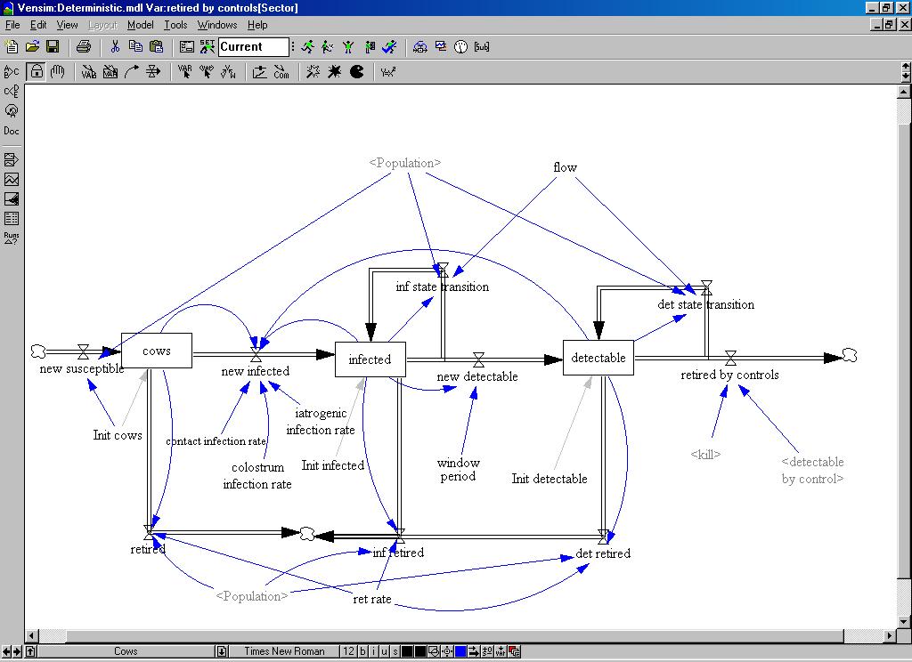
Figure 4. The structural diagram of the system dynamics model

5.11

As we have already said our model is not a pure SI model but we have a flow of retired subjects, these are the infected dairy cows detected during scheduled controls. All detectable cows are butchered in a single day, the unit time of our model, so that the retired is a pulse function, whose schedule depends on actual sanitary warranty and the previous number of detectable subjects, and whose amplitude depends on the previous number of detectable subjects.

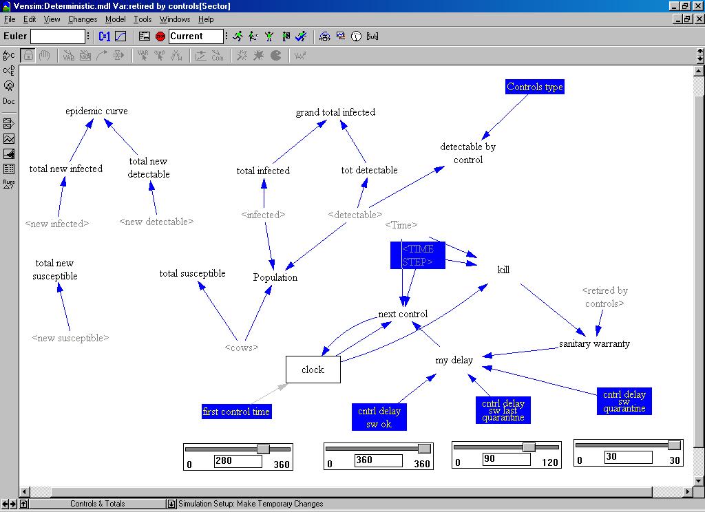
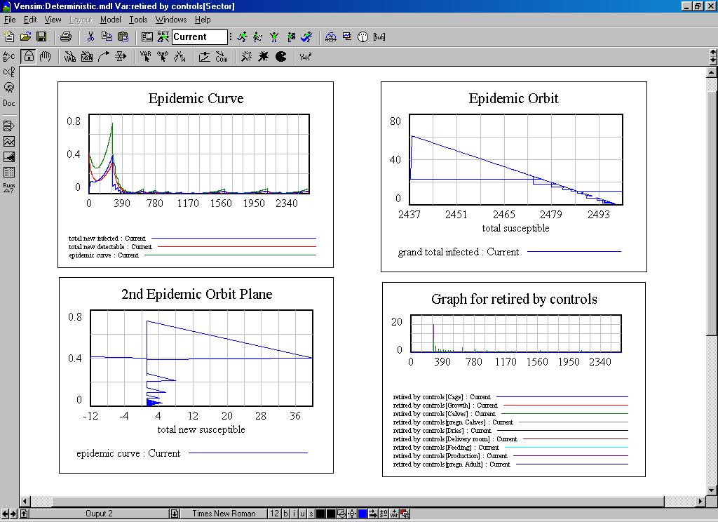
Figure 5. The controls and totals in the system dynamics model

5.12

The iterative solutions describe our dynamic system and a series of graphs depict the disease behaviour:

1. susceptible, infected, detectable subjects for each sector;
2. the epidemic evolution for the whole farm;
3. the epidemic curve, that is the derivative of infected and detectable subjects;
4. the epidemic orbit projections: these are the projections on two-dimensional surfaces of the infection represented as a point in multidimensional phase space, in other words it is a snapshot of the dynamic behaviour of the whole system so that the stability or instability of the system may be seen at a glance;
5. the number of retired subjects due to scheduled controls.

5.13

As a sample we reproduce the results of a typical deterministic run. The first map represents: susceptible, infected, detectable subjects for each sector and the epidemic evolution.

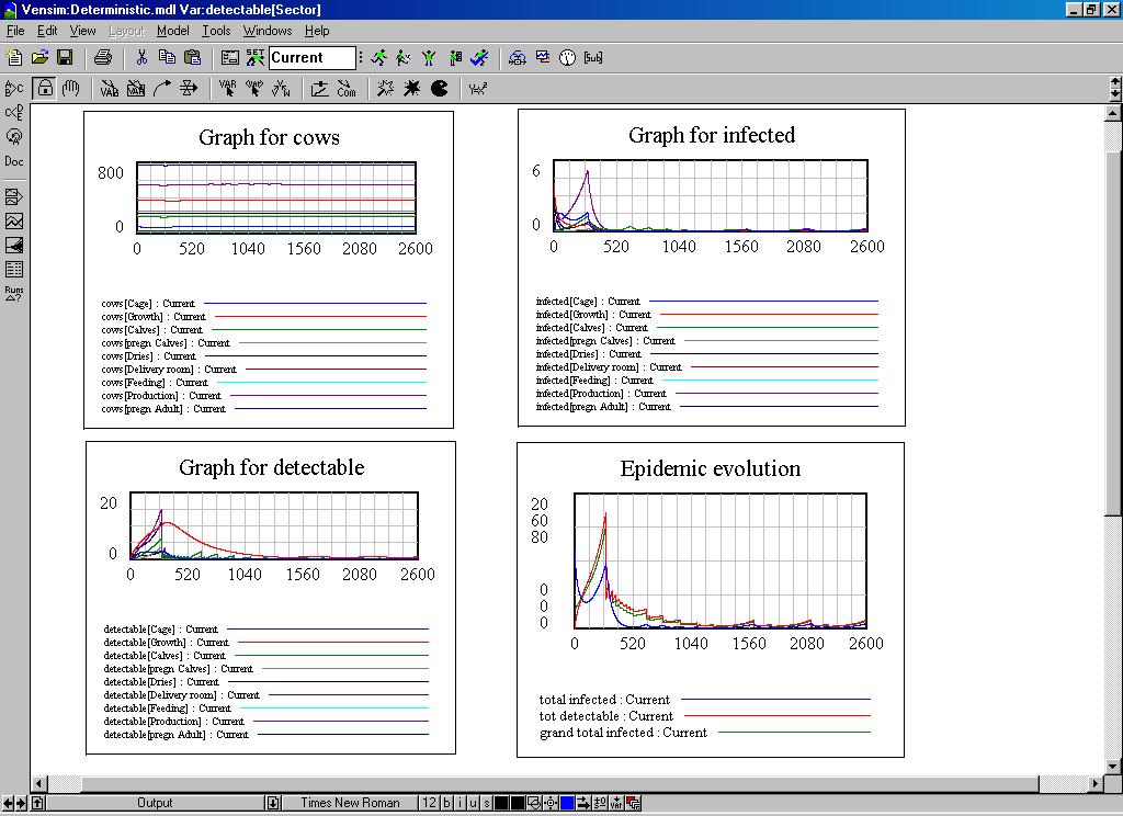
Figure 6. Some dynamic graphs of the system dynamics model

5.14

The second map depicts the epidemic orbits and the number of retired due to sanitary controls.

Figure 7. The behaviour of the system dynamics model

5.15

At the moment we are also implementing a stochastic model, with integer variables, whose expected values are obtained from the deterministic model. We apply random oscillations around every stock and flow variable, we then use the integer output as input for related flows or stocks so that we can obtain a reasonable stochastic behaviour.

"Agent Based" specific points of view

5.16

As an alternative to the System Dynamics we have decided to develop another simulation model that allows a refinement of the analyses of events that involve the animals in the farm in order to view the complexity and non linearity of the system under investigation from a different perspective.

5.17

Agent-Based modelling entirely meets these requirements, allowing the passage from the difficulties arising in the formalization of the complex equations that describe the systems to the more natural and simpler description of the properties and behaviours of their parts.

5.18

The simulation model use the Swarm environment, a collection of libraries written in "Objective-C" which provide support for the design of an agent-based model and facilitate the management of technical issues like scheduling of actions, maintenance of lists, drawing of graphical objects and so on. Is also possible to write the model in Java, accessing its routines through a specific layer (Java Native Interface). We have explored both solutions.

5.19

A typical Swarm application is hierarchically structured in levels. First, there is a top-level, called "observer swarm", that creates screen displays and also creates the level below it, which is called the "model swarm" (possibly containing other "model swarm" in a recursive manner), that creates the individual agents, schedules their activities, collects information about them and relays all that information according to the observer's requirements. Finally, agents are present and if necessary, other levels, each one built by the "model swarm" and provided with own properties and methods (Johnson and Lancaster, 2000).

5.20

The translation of an identified scheme in an agent-based model has required the definition of the agents and the events of the system, according to the object-oriented paradigm. Therefore, it has been necessary to determine the characteristics (properties) and the behaviours (methods) of the objects and to gather them in modular units (classes) which are hierarchically related and capable of communicating between each other by messages. To accomplish this task, we relied on UML diagrams built in the conceptual phase.

5.21

In detail, we have defined four classes: one that represent the cows of the dairy farm, one for the sector that constitutes the farm and the other two to meet the architectural requirements of the Swarm platform. It is important to notice that the "model swarm" carries out the typical function provided for the platform, but it also can be viewed as the representation of the entire farm because it records their parameters (total number of cows, sanitary warranty and so on).

5.22

Concerning the "cow" objects, we have defined several properties to record the registry data of cows, their state of health and their position in the farm.

registry data	state of health	position in the farm
sex	state	arrival time at the farm
birth time	infection time	arrival time in the sector
insemination time	infection factor	spatial coordinates
pregnancy	disease detection time	actual sector
number of deliveries	the state of health of the mother (at parturition time)	colour of the cow, to visualise the state
last parturition time

5.23

These properties allow one to determine the animal's life cycle inside the logistic structure of the farm, where the shifting of the animals between the sectors are related to specific events (birth, insemination, parturition) and where their duration of life depends on the number of parturitions they endure.

5.24

Moreover, it is possible to fully trace the evolution of the clinical state of each animal. We can find out, all through the simulation, in detail, whether a cow is healthy or infected (detectable or not)^[4], if it is infective for the other animals and the eventual time and cause of infection.

5.25

We also implemented the methods of "Cow" class that permits one to read/write the properties of the objects and to simulate the changes of state and the actions that involve the cows (for example, delivery, contagion and sanitary control).

5.26

In the "model swarm" level, we take the actual characteristics of the farm into account (total number of cows and sectors, sanitary warranty, etc.) and, according to the features of the platform of simulation used for the management of the objects and their activities, we also organized the agents in lists to facilitate their manipulation.

5.27

The flow of cows from one stock to another or from a sector of the dairy farm to another one is a task accomplished in the "model swarm"; generally speaking, here we have the definition and the scheduling of the events that can occur during the life of the animals, including those related to the spread of infection. Therefore, at every step of the simulation, the situation of the cows is verified, and timely action may be carried out when certain conditions are found. These are generally related to the time of permanence in the specific sector of the farm taken. Change of sector and a change in the state of the animals (birth, insemination, parturition, death, etc.) are possible measures that may be taken.

5.28

We have kept the number of dairy cows in the farm stable, or at least in the neighbourhood of the established target, simulating the selling of males (within eleven days from birth) and of exceeding calves.

5.29

Furthermore, we have implemented an initialization routine to populate the model with agents whose conditions reflect a typical situation of the farm. The key assumption here is that the population is uniformly distributed regarding age, and hence every agent of the model is 'aged' with a random value included between 0 and the maximum possible (about 2000 days). From the age assigned, the other attributes of the cow were derived according to the fact that the life cycle is strictly regulated by periodic events. The initial infected agents are also opportunely set up randomly according to the number specified, or directly by experimenters using 'probes' to control the single agent and hence decide what specific cow must be set as 'infected' at every step of the simulation.

5.30

Concerning the means of contagion, we have simulated mother-offspring, contact, infected milk and palpation for every single agent; a potentially dangerous event (birth, nursing, examination) can determine an effective contagion with frequencies conforming to the estimates of the experts. In particular, the availability of lists of agents has been fundamental to the implementation of both nursing and gynaecological visits (for instance cows were randomly selected from the list and were examined in sequence with the same palpation sleeve.)

5.31

The model carries out sanitary controls, together with relative effects on the sanitary qualification of the farm. Since the time when controls are made is not preset, we are facing an asynchronous event driven problem. We have used the 'dynamic scheduling' technique that enables the planning of a group of actions dependent upon specific events. In detail, after a sanitary control has been carried out on the farm, we verify the result of this and the situation of the farm following the previous checks to determine any changes to be made to the sanitary qualification of the farm and to schedule the next control. The following table summarizes all permissible combinations of the farm's parameters and the test results (on the left) and the corresponding effects on the farm's state and the scheduling of the next sanitary control (on the right).

Farm's Parameters		Test Result	Effects		Next test Interval[5]
Quarantine	Last Test Interval		Qualification	New Quarantine
NO	Normal	Negative	YES	NO	Normal
NO	Normal	Positive	NO	NO	Very Short
NO	Very Short	Negative	NO	YES	Short
NO	Very Short	Positive	NO	NO	Very Short
YES	Short	Negative	YES	NO	Normal
YES	Short	Positive	NO	NO	Very Short

5.32

The resulting general structure of the simulation is as follow:

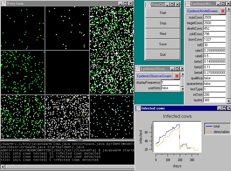
Figure 8. The structure of the agent based simulation

5.33

Finally we have created the graphic widgets required for interaction with the user and present the collected information in the higher level of Swarm architecture, the "observer swarm":

1. a control panel that contains a set of buttons that can start, stop or 'step' the simulation and save the window position of the object;
2. a bidimensional grid in which all the agents are represented with different colours depending on their state; the division of the farm in sectors is also represented;
3. a graph displaying the total number of infected subjects (it is the integral of the "epidemic curve") and the number of infected cows that are already detectable at sanitary tests;
4. a histogram with the current number of cows for every sector of the farm;
5. a command-line window, from the model is started and where information about some simulation quantities is displayed (e.g. the number of cows detected during a clinical test of the farm);
6. a series of 'probes', that supply a graphical snapshot of the object of the simulation and that allows the updating of their parameters.

5.34

A comprehensive view of the GUI of our model during a typical run is reproduced below:

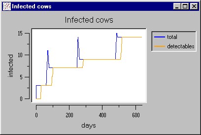
Figure 9. A simulation experiment in the agent based model

Model calibration and validation

6.1

In order to obtain a valid and helpful model with which epidemiologists can perform an interpretation of an actual situation the model must, first of all, be calibrated correctly.

6.2

The question of the evaluation of parameters is closely linked with the problem of the validation of the model: even if we have a well designed model but incorrect parameters, our model will not fit the target (real world). If, on the other hand, we are not able to find an exact data fit, this may be an alarm signal indicating a poorly designed model.

6.3

As previously described, the structural parameters of the model follow the organization of a typical Italian dairy farm. On the other hand, the values of epidemic parameters have been inferred by current scientific literature, from the experience of researchers and from data results gleaned from the field. We must admit that these estimations are actually subject to an ample range of error. We have not used, initially, a mathematical statistics approach to validate the model due, also, to a scarce availability of real data from the field.

6.4

Instead, we have adopted the "weaker criterion", comparing the results of model with the experts' empirical knowledge of the system behaviour (in reference literature this is also called 'face' validation). To accomplish this task, we have made massive use of the dynamic graphical plots provided by both of the models.

6.5

In particular, the subject-matter experts checked the distribution of the cows in the sector, the movements inside the farm and the epidemic dynamic. This kind of analysis determined an iterative process where the parameters of the model were 'tuned'.

6.6

Recently, we have achieved a more stringent degree of assessment by testing the model quantitative agreement with data from the real world. We have used available real data of infection spread on a farm and we have compared it with data from the model. Using some of the features of Vensim software, especially optimisation and "goal seeking", we were able to find the parameter values that minimize the overall Mean Square Error, when conducting a first verification of the hypothesized infection rates.

6.7

The accordance between estimated preliminary infection rates, using the model, and those reported in current scientific literature as a result of experimentation, is very strong. Thus we can deduce that the map of organizational structures of the farm and the infection issues of our model are satisfactory. Unfortunately this kind of "reverse evaluation" of model parameters, at the moment, is possible only for "System Dynamics models", because the agent based development tools do not have built-in features of this kind.

6.8

However, more precise hypotheses and their validations will only be possible by using a model whose parameters have a smaller range of error. We can develop a further evolution in this sense only by collecting more data from the field in order to compare model outputs with time series data gathered from different real farms.

Simulation experiments

7.1

The tuning of the model was focused particularly on the number of cows detected as positive at sanitary controls. This quantity differs from the total number of infected on the farm, which would be more useful for the expert to know but this data is not available due to the presence of silent and subclinical cases^[6]. The simulation models can offer an important aid in this situation because they supply an estimate of the total number of infected on the farm at every time step of the simulation.

7.2

The first results of the analysis conducted on this subject gave some important indications to the experts, above all concerning the infected animals that the current sanitary controls are not able to discover either because of the intervals between two following tests or due to the serum-conversion process. The knowledge of the characteristics of these cows is the starting point to hypothesize changes in the organization and in the modality of the sanitary tests.

7.3

Moreover, the constructed model allows the user to regularly monitor the simulation by means of a series of graphs, as well as to customize experiments by changing characteristic quantities of the system at the initialization step or, for "Agent Based Models" only, altering the agent characteristics at any moment, using the so called "probes". Thanks to these facilities, the experts have conducted a sensitivity analysis to determine how the specific model factors have a significant impact on the overall model's behaviour.

7.4

In particular, in the model, the spread of the epidemic due to palpations is rather slow when there are few infected cows, but it suddenly changes when there are many sick animals. A great number of infected animals are located in the 'production' sector, where simulated palpations and injections are more frequent.

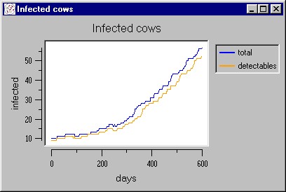
Figure 10. A simulated epidemic waves caused by the palpation/injections factor

7.5

Instead, transplacental transmission at the moment of parturition and the administration of colostrum exhibit a trend which is less dependent upon the number of infected subjects because the model's assumption is that a single sick cow can contaminate several young calves. Hence the simulations bring to light the fact that these mechanisms, in particular contamination through colostrum, appear critically important as they can 'restart' the epidemic even when the presence of infected dairy cows is scarce.

Figure 11. A simulated epidemic waves caused by the vertical forms of transmission

7.6

Although the system is globally stable on a long term basis, a small initial shock (4 infected animals) is sufficient to provoke a quick spread that controls are able to halt only after 1100 days circa. This looks as if it is due to the actual structure of the sanitary controls themselves which fail to locate infected young calves, allowing them to spread the epidemic between two successive tests, making the infection endemic. During this period, such animals may be sold to other farms thus starting up a new epidemic process.

7.7

The most evident improvement in the use of the simulation is the availability of conspicuous quantities of artificial data, which is hardly ever obtainable in the real world because of the elevated costs of polls or the rarity of phenomenon. This has allowed the experts to do a preliminary "what-if" analysis with the purpose of assessing the system's behaviour under different conditions and evaluating which alternative policies to adopt. The "Zooprofilattico" Institute researchers have hypothesized that disease may be endemic due to the failure of current methods of control to identify the very young infected calves, which can start a new spread of infection between one control and the following. Based on this observation, they are devising new kinds of "virtual" controls to test them in the simulation environment.

Conclusions and further developments

8.1

Finally we would like to illustrate and outline the difference between the Agent Based and System Dynamics technique and archetype not only from a theoretical viewpoint, which has already been amply dealt with in many books, articles, and manuals about computer simulation, but from the perspective of the researcher, whose target is to tailor model as far as possible in accordance with the real situation.

8.2

Our conclusions refer to the models developed for the specific case study previously explained in the article.

System dynamics

8.3

As already outlined, we can see the System Dynamics Modelling as an extension of the time dependent systems of differential equations, a traditional technique which has been consolidated and well tested. As a consequence we can find products that solve the problem and which also provide an assortment of tools.

8.4

Our impression is that System Dynamics models are particularly useful for pinpointing the highways of infection spread and sketching the overall framework of the model. Thanks to their graphical facilities, it is easy to build up models from scratch, to maintain models, or to change scenarios and to explore what happens if the model mutates its structure due to a great shock or to environmental changes. In our case study, this characteristic allowed the rapid development of a basic model which has greatly improved interaction with the experts during the early stages of the project.

8.5

Furthermore, we took advantage of the availability of built-in features like optimisation and "goal-seeking", which are not present in the agent-based platform, in order to calibrate the parameters of the model and to verify their accordance with reference material.

8.6

However, we must underline the well known limits of this approach: the target is depicted as a whole and it is impossible to design the fine structure of the model so that even important behaviours of model components are lost in the overall evolution. In our study we observe that all variables are "smoothed", for instance it is not possible to observe the described "transition phase" as in the agent-based model.

Agent Based Modelling

8.7

The chance to work on agents and on their artificial world has been of enormous importance for a correct sketch of our problem. The definition of agents, of their states, and of the virtual world in which they can act, almost automatically lead to a representation which is closer to reality.

8.8

Our utilisation of the agent-based technique is a little different from its canonical use in social sciences, where the agents can perform in an autonomous manner, because the system we investigated exhibits a remarkable complexity due to the strict organisational aspects of the farm and to the multiplicity of the infective factors and their interactions. The originality of our work resides in the implementation of agents which act (and interact) in a context governed by strict rules related to specific events.

8.9

This specific requirement has not lessened the benefits of implementing actions at the agent level, which is not possible with other approaches like differential equations and system dynamics. In particular, we can indicate means of contagion such as palpation and contact (the latter showed itself as not being significant during simulation) that we set up respectively, using the option of managing the single agents grouped in lists, and considering the spatial factors involved in the spread of disease.

8.10

The simulation model which we implemented exhibits a peculiar characteristic of agent-based paradigms, that is the emergence of a complex behaviour. In particular, in comparison with quite simple behaviours of the agents, even if they are included in a well-defined context, the overall dynamic of the system appears very complex and strictly sensitive to the initial conditions. We took advantage of this characteristic to evaluate the impact of changes at micro-level on the entire system.

8.11

On the other hand, the implementation of the agent-based model requires a significant amount of programming compared with the visual approach allowed by system dynamics tools. Moreover, at this time, agent-based platforms do not offer functionality that can aid the calibration of the parameters.

8.12

It is important to remark that the agent-based models may be further developed, and these are more promising and simpler to produce than other approaches thanks to their "open source" structure that allows integration with other tools such as statistical software and GIS packages.

Further developments

8.13

The main evolutionary lines of the project - involving mainly the agent-based platform - can be pointed out as:

• to generalise the representation of the farm, allowing the user to differentiate dimension, organization issues and operational structures;
• to conjugate the new control policy devised with economic issues to check its real feasibility and to fully compare alternatives;
• to proceed from a "mixed" model, with deterministic state transitions of agents and random epidemic diffusion, to an entirely stochastic model with all the agents heterogeneous. This requires the analysis of the random distributions of quantities that characterize the cow (duration of life, number of necessary inseminations, etc.);
• to develop a batch model which reads external parameters so that we can do repeated runs with the sampling of data and use the R language for statistic analysis on model outputs.

8.14

Thanks to enormous potential of Agent Based tools we can also hypothesise more substantial developments like, for instance, reasoning in terms of farms and not of cows using GIS tools to plot the epidemic evolution on the land, or applying these new techniques to other types of infection.

Acknowledgements

The authors are grateful to Giancarlo Ferrari, Marcello Sala and Gaia Scavia of the epidemiological observatory of the "Istituto Zooprofilattico Sperimentale delle Regioni Lazio e Toscana" for their invaluable contributions and for the precious discussions.

Notes

¹ Specific study have highlighted the importance of an opportune and effective individuation of infected animals, estimating that the percentage of serum-positives drop down from 95% to 34% in three years when sick cows were systematically separated from the others (Sargeant 1997).

² The Unified Modelling Language (UML) is a language for specifying, visualizing, constructing and documenting the artefacts of software systems, as well as for business modelling and other non-software systems. The UML represents a collection of the best engineering practices that have proven successful in the modelling of large and complex systems.

³ that is the resistance to contract the infection following exposure to infective factors.

⁴ Note that the state "detected infected" is not needed because cows that have a positive result at a sanitary test are immediately separated from the others, even if they are butchered a few days after.

⁵ Note that, according to the Italian policy for the bovine leukemia control, we have roughly approximated these intervals assuming that when the farm doesn't exhibit cases of infection, the sanitary test are scheduled every year (normal interval), while a test with at least a positive animal determine a following test after two months (very short interval) and the quarantine period is about four months (short interval).

⁶ In the medical literature, this is called the 'Iceberg Principle'.

References

BAILEY N.T.J. (1975) The Mathematical Theory of Infectious Diseases and its Applications II ed., Griffin & Co.

BANKS J. (1998) Handbook of Simulation: Principles, Methodology, Advances, Applications, and Practice. John Wiley & Sons.

BARTLETT M. S. (1960) Stochastic population models in ecology and epidemiology. Methuen, London.

BILLARD L. (1973) Factorial moments and probabilities for the general stochastic epidemic. J. Appl. Prob., 10, pp. 277-288.

BOOCH G. (1999) The Unified Modeling Language User Guide. Addison-Wesley.

ELVEBACK L., Ackerman E., Gatewood, L. and Fox, J.P. (1971) Stochastic two-agents epidemic simulation models for to community of families. Am. J. Epidem., 93, pp. 267-280.

ELVEBACK L. (1971) Simulation of stochastic discrete-time epidemic models for two agents. Adv. Appl. Prob., 3, pp. 226-228.

EWY W., Ackerman E., Gatewood L., Elveback, L. and Fox, J.P. (1972) To generalized stochastic model for simulation of epidemics in to heterogeneus population (model You). Comp. Biol. Med., 2, pp. 48-58.

FORRESTER J.W. (1961) Industrial Dynamics, The MIT press.

GALLOP R. J. (1999) Modeling General Epidemics: SIR MODEL, Proceedings of the 12^th Annual NorthEast SAS⁽ Users Group Conference.

GANI J. (1969) A chain binomial study of inoculation in epidemics. Bull. I. S. I., 43(2), pp. 203-204.

GANI J. and Jerwood, D. (1971) Markov chain methods in chain binomial epidemic models. Biometrics, 27, pp. 591-604.

GILBERT N. and Troitzsch K. G. (1999) Simulation for the Social Scientist. Open University Press.

HOPPENSTEADT F. (1975) Mathematical Theories of Populations: Demographic, Genetics and Epidemics. SIAM Regional Conference Series in Applied Mathematics 20.

JOHNSON P. and Lancaster, A. (2000) Swarm User Guide http://www.swarm.org

KERMACK, W.O. AND MCKENDRICK, A.G. (1927) Contributions to the mathematical theory of epidemics. Proc. Roy. Soc., To 15, (Part I, 1927).

KENDALL D.G. (1956) Deterministic and stochastic epidemics in closed populations. Proc. Third Berkeley Symp. Math. Statist. & Prob., 4, pp. 149-165.

LAW A.M. and Kelton W.D. (2000) Simulation Modeling and Analysis, Third Edition. McGraw-Hill.

LUNA F. and Stefansson B. (2000) Economic Simulations in Swarm, Agent-based Modelling and Object Oriented Programming, Kluwer.

RENSHAW E. (1991) Modeling Biological Population in Space and Time. New York, NY: Cambridge University Press.

RITCHIE-DUNHAM J.L. (1995a) Application of Systems Thinking in the Mexican Health Sector: An Epidemiological Case Study of Decision Policies in Combating Hemorrhaging Dengue, Third International Decision Sciences Institute Meeting, Puebla, Mexico.

RITCHIE-DUNHAM J.L. (1995b) "Evaluating Policies/Strategies to Combat Epidemics with Systems Thinking", http://www.sdsg.com/new/appbntrf.htm

SARGEANT J. M., KELTON D.F., MARTIN S. W. AND MANN E.D. (1997) Association between farm management practices, productivity, and bovine leukaemia virus infection in Ontario dairy herds. Preventive Veterinary Medicine, 31.

SWARM DEVELOPMENT GROUP (2000) Swarm 2.1 Reference Guide, http://www.swarm.org.

Return to Contents of this issue

© Copyright Journal of Artificial Societies and Social Simulation, [2002]