The spatial pattern as described by von Thünen is considered an optimal solution to maximize society's well-being in a hypothetical environment. We developed a model to demonstrate whether a collection of autonomous individuals can contribute to the formation of this optimal pattern, without any system-level optimization capabilities. We also analyzed the mechanism that leads to an emergent spatial optimization by applying theories of positive feedbacks and lock-in.

Keywords:

Emergent Optimization; Lock-In; Positive Feedbacks; Spatial Constraints; Swarm; Von Thünen's Isolated State

Introduction

1.1

In 1826, Johann-Heinrich von Thünen, an educated landowner in northern Germany, published a treatise, Die isolierte Staat in Beziehung auf Landwirtshaft und Nationalökonomie (Wartenberg 1966; von Thünen 1926), which became one of the founding works in spatial economics and location theory. In this work, von Thünen gave a predictive model of rural development around an idealized isolated urban center, imposing several simplifications in an attempt to focus on some of the fundamental processes at work in settlement patterns and rural economic activity. It is presently a regular component of introductory economic geography courses. Despite criticisms for oversimplifications, it has persisted in geographic, economic, and rural development curricula.

1.2

Von Thünen emphasized that his findings had no claim to universality (Chisholm 1981), but were meant as generalizations towards discovering laws which govern agricultural prices and translate them into land use patterns. Peet (1969) correctly compared this process of generalization to creating a laboratory in which the interplay between a small number of processes could be studied, and causal mechanisms between economic inputs and geographical patterns could be explored. The history of the debate over von Thünen's ideas in geography and economics is extensive and will not be reviewed here; for such a review see Block and DuPuis (2001).

Table 1: Generalized agricultural categories in von Thünen's scheme
I	Intensive Agriculture	Fruits, vegetables, and dairy; products that perish quickly and must be transported immediately to market.
F	Forestry	Woods, both for construction and firewood. In von Thünen's time these were the primary sources of energy and a daily necessity within the city.
G	Grain Farming	Grain and staple production.
L	Livestock	Ranching and animal husbandry for meat, hides, and other non-dairy products.

1.3

Von Thünen considered four generalized types of economic and agricultural activities, categorized according to relative economic yield per unit area and perishability or difficulty of delivering products to market (table 1, in an order of roughly decreasing perishability and yield per land area). He made predictions of the distributions of these activities relative to an isolated urban center. Assuming an otherwise homogeneous landscape (equal fertility and access to water throughout the area) and isolation of the system (no trade connections with outside states), von Thünen theorized that the following three factors would affect the spatial distribution of agricultural types:

• More perishable products would be grown closer to market
• Products with higher economic productivity per land area will be grown closer to market
• Products that are more difficult to transport will also occur closer to market.

1.4

According to these assumptions, one would expect that different types of agriculture will form in concentric rings around the market, ordered in distance from the center according to their relative values of the three factors mentioned (figure 1).

Figure 1. von Thünen's isolated state

1.5

Von Thünen's approach was considered in terms of global properties of a city and surrounding areas. The assumptions listed before are instrumental in maximizing efficiency and minimizing overall costs to the city as a whole. A rural planner who buys into this theory might be tempted to effect maximum efficiency through land zoning or some other centrally imposed order. However, most of the forces attributed to creating these conditions occur from the bottom up, and much of what is observed as a global pattern is in fact the emergent result of many individual actions.

1.6

It is not readily apparent to everyone how a society composed of such selfishly motivated participants, bereft of any higher motivation and lacking any centralized authority, could produce a market that spatially conforms to von Thünen's idealization, which gives an optimum solution for society in terms of overall costs and efficiency. It is tempting to think that a combination of extra factors that would accompany any real city, with social relationships, governments, competing urban centers, wars, etc., would be a necessary ingredient to shape these individuals into the most efficient pattern. An alternate explanation, which von Thünen espoused, is that this spatial optimization can occur spontaneously through the interactions of selfishly motivated individuals, without any external forces working on them. The spatial optimization is in fact an emergent phenomenon of the individuals' interactions, as described in popular books such as Holland (1995) and Axelrod (1984). Our objective in this study is to gain some understanding as to how individual actions and motivations can translate into a global pattern such as that predicted by von Thünen. More specifically, can the simplified assumptions stated in the preceding paragraphs, acting at the individual level, produce a global pattern as von Thünen predicted?

1.7

If we create a world with the homogeneity that von Thünen envisioned, and populate it with selfishly motivated individuals who react to nothing other than market forces subject to spatial constraints, they should be able to create the pattern in figure 1. Our approach in this study is to model the fundamental processes of micro-scale economics (which is goal-based rather than utility-based) at the individual level, implement that model in an individual-based simulation (agent-based model, or ABM), and examine emergent global properties of a city that comes from these individual actions. Assuming that each economic agent is selfishly motivated to minimize his/her costs in an attempt to maximize profits, altruistic cooperation with other agents for the global good of the system is not considered to be part of the individual's decision process. For example, a livestock farmer, who's land needs are high, per acre productivity low, and transport costs are cheap, would ideally have land further away from a market than farmers in the other agricultural categories; however, if an individual livestock farmer is able to acquire land closer to market for a reasonable cost, it's reasonable to assume that the farmer will want to acquire that land thinking of his or her own economic gain. Personal economic considerations will probably outweigh any altruistic notions of what kind of farmer would best be suited for the land. This does not mean that the agents' actions contradict von Thünen's and other researchers' assumptions, as the mechanism by which micro behaviors translates to macro structures has long been explained.

1.8

This study is not meant to be a predictive model per se, as ABMs are not particularly well suited for empirical prediction. ABMs are most useful for studying the mechanisms by which simple rules translate into complex emergent phenomena (Axelrod 1997); this study is meant to document a set of conditions by which simple rules at the individual level can translate through multiple feedback into the concentric rings von Thünen envisioned.

Previous Work in This Area

1.9

There have been several studies that have used ABMs to model land-use patterns, where autonomous agents effect change in localized patterns of land according to economic and agricultural properties of the land. This technique has been used to recreate population patterns in prehistoric settlements given known properties of landscape productivity and climate records, including Kohler et al. (2000), Kohler and Van West (1996), and Dean et al. (2000). It has also been applied to modern agricultural societies such as rural Brazil (Lim et al. 2002) and Mexico (Manson 2000). They have proven useful as a method for evaluating policy (such as Antona et al. 2002 in Niger). Other existing studies have provided insight into how social interactions and varying amounts of information about the surrounding world give rise to important dynamics (Deadman 1999 is a good example), and Otter et al. (2001) gives useful insights into economics and emergence of land use patterns (residential and commercial agglomeration) through ABMs, and used von Thünen's theory as part of the foundation of their work. However, von Thünen's predictions seem to have never been explicitly investigated by applications of these techniques.

1.10

Parker (2000) used economic behavior in autonomous agents who were fixed to their cellular locations to investigate emergent spatial land patterns, and had noted von Thünen's patterns emerging in some simplified cases. Notably, transportation costs alone were sufficient to produce a unique equilibrium that conformed to von Thünen's predictions. Many studies have applied CA techniques in land use studies, especially in urban growth simulations (Clarke et al. 1997 is a notable example); however, strict CA rules impose a constraint of stationarity on the agents, that might be considered unrealistic. Several papers (Box 2002; Manson 2000; Bousquet and Gautier 1998) propose methods for hybrid CA and ABM approaches, and Torrens and O'Sullivan (2001) make an argument for such; however, given the self-interested nature of the agents that we wished to investigate, there was little justification to give decision-making power to the land itself, nor was any justification to bind agent's too tightly to a particular land parcel.

1.11

The purpose of this study is to investigate how economic forces affect individuals to adopt practices that could create a spatial pattern. In this respect, we will adopt similar economic feedback patterns as are proposed in Parker (2000) and Torrens and O'Sullivan (2001), but with mobile agents whose ability to conduct their economic activity are constrained by space.

Some Theoretical Background

2.1

By explicitly modeling micro-scale, or individual level actions, we expect that a few well-understood economic forces will combine with spatial location to collectively produce a global pattern. We will represent the assumptions in section 1 as two forces that fundamentally affect the location of an agricultural producer relative to market. One is a force that encourages agricultural producers to be closer to market (F1). This is defined by the perishability of the product and the producer's desire to minimize transportation costs. Fruits and vegetables are highly perishable and difficult to transport, so farmers with this type of intensive agriculture are particularly motivated to grow their crops closer to market. A second force (F2) encourages farmers to locate further away from the market. This force is defined by the availability and cost of land closer to market. Livestock farming is less economically productive per unit area of land than intensive agriculture, and thus requires more land to be viable. Additionally, in von Thünen's time, livestock were self transporters, making them much easier to deliver to market over longer distances than fruits or vegetables. If the assumptions in section 1 hold, these forces should conspire to force intensive agriculture closer to market and livestock production further away.

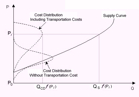
Figure 2. Cost distributions of commodity with and without transportation included

2.2

In addition to location, economic forces should play a major role in forming von Thünen's rings. If one plots the cost distribution of a commodity, which is the amount of the commodity that can be produced at a given price P_i, one should get a normally distributed curve, which is plotted on the P axis in figure 2. If additional transportation costs are added to these costs, the distribution of P_i will be skewed, shifting it to higher values of P. The shifted distribution curve indicates the quantity Q_CDf(P_i) that can be produced at the new P_i. Taking the integral of this distribution curve over P generates an estimate of the supply curve:

(1)

where Q_Sf(P_i) is the cumulative quantity on the supply curve on P_i and Q_CDf(P_i) is quantity of the cost distribution P_i. This is more appropriate for our study than the standard theoretical method of calculating supply, where one calculates the marginal cost curves for all individuals in the population and adds them together. For computational efficiency, we are considering the state as an individual producer, and approximating the supply curve this way for reasons that should become apparent in section 3.3.

Figure 3. Conditions forcing an increase in equilibrium price

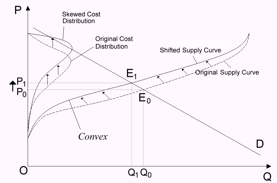
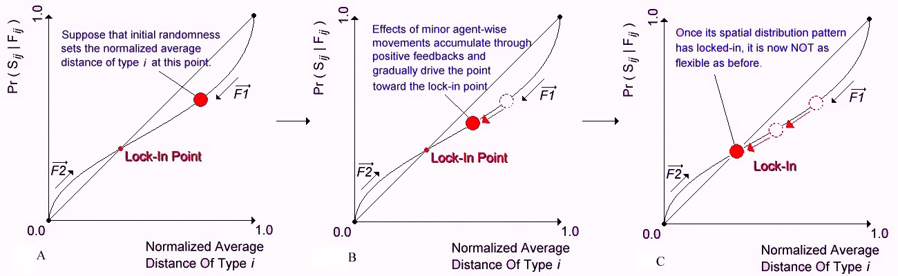
Figure 4. Increase in cost curve causing increasing equilibrium price. Feedback results in convex shape of curve at lock-in

2.3

The interaction between equation 1 and with the forces F1 and F2 should play out in the following way in space: relatively weak F1 and/or stronger F2 would cause agents who are closer to the market to shift their activities to land that's a little farther away from market. That would shift the supply curve up a little bit, causing a slightly higher equilibrium price (figure 3). While the shift may be negligible, the slightly higher equilibrium price allows farmers to pay slightly higher transportation costs. With that, the farmer will be a little more likely to acquire a larger area of land further from market in the face of a scarcity of closer land. This then causes a further shift upwards of the supply curve, followed by another upward shift of the equilibrium price. This gives a positive feedback which magnifies the micro-scale activities of individuals to effect a macroscopic tendency (figure 4). Conversely, a relatively strong F1 and weak F2 would have individuals locate closer to market, shifting the supply curve a little downward and causing a slightly lower equilibrium price (figure 5). This is also magnified over time through positive feedbacks.

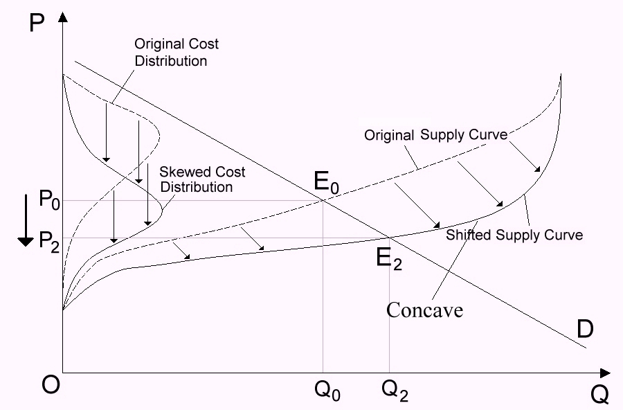
Figure 5. Conditions forcing a decrease in equilibrium price

2.4

The feedback process described in figure 3 effectively pushes agricultural fields away from the central market; this is especially notable in livestock farming since that requires a larger area of land and is subject to a relatively strong F2. The other feedback process described in figure 5, is more typical of intensive agriculture, since its products are highly perishable and subject to a stronger F1.

2.5

These positive feedbacks might continue indefinitely, though that does not happen in reality nor in theory. There is "lock-in" point for each activity type, described by Arthur's idea of the non-linear Polya process (Arthur 1987, 1990), where, in our case, the positive feedbacks yield a balance between economic and spatial forces that eventually produce an inflexible state. The assumptions and objectives of Arthur's work are described for a different context; however, they seem applicable here by the following argument:

2.6

Let F_ij be the event that the j^th farmer of type i settles down in the hinterlands at a specified distance from the central market. Let S_ij be the event that the j^th farmer of type i succeeds in his/her agricultural enterprise. i has four possible values, representing the four types of agriculture in table 1. The notation Pr(S_ij | F_ij) represents the probability of success by the j^th farmer of agricultural type i, given the condition that s/he has settled at the given distance from the market. This conditional probability is assigned to the y value, and the average distance of fields of agricultural type i from the central market normalized by the maximum possible average distance is assigned to the x value; x, y ∈ [0, 1]. Since the conditional event (S_ij | F_ij) is the mechanism to increment the normalized average distance of type i, there is a positive regression relationship where y is roughly the cause of x. Also, the conditional probability (y) is a function of the normalized average distance (x), because a greater x brings about a higher equilibrium price and (S_ij | F_ij) is more probable for reasons discussed previously. Therefore, x and y have mutual cause and effect relationships. For any agricultural type i, the result of the positive feedback follows the curve defined by y = f_i(x) which represents a slight deviation from the line y = x. Theory says that a lock-in point exists at the intersection of the curves y = f_i(x) and y = x for each i. Let the coordinate of this lock-in point be (x_li, y_li). The stochastic relationship between x (normalized average distance) and y (Pr(S_ij | F_ij)) can be summarized with the following motions:

• MOTION 1: if y < x; positive feedbacks likely to decrement x and y
• MOTION 2: if y > x; positive feedbacks likely to increment both x and y

2.7

Additionally, dy/dx decreases as current point nears lock-in point. These two opposing motions are associated with the two space-driven forces F1 and F2 discussed earlier. A relatively strong F1 and weak F2 is found when y < x and x > x_li, and the reverse is found when y > x and x < x_li. This process is illustrated in figure 6. MOTION 1 is shown in figure 6A, with strong F1 and weak F2. With Pr(S_ij | F_ij) smaller than the normalized distance, farmers of agricultural type i who are farther from the market are more likely to fail, and the average distance of fields of type i would shrink. Despite an initially wide spatial distribution of fields and agriculture types (random x), the combination of F1 and F2 should produce a lock-in (x_li, y_li). If one follows the average distance of fields with a given agriculture type over time (figure 7A), one would see an initially random trajectory of this distance, with a fairly noisy look about it as the average distance fluctuates. Over time, however, one would see the trend move towards a straight line (constant value), with a much less noise (a sign of decreasing dy/dx as x,y → x_li, y_li), with the trend settling on the lock-in price over time. As these average distances are distinct from each other, one would expect that the spatial arrangement would look like von Thünen's rings (figure 7B.)

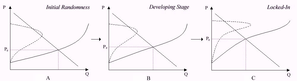
Figure 6. feedback from individual agents causing lock-in of price

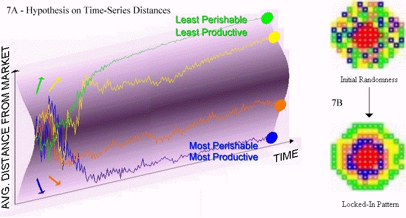
Figure 7. Lock-in of prices represented in time and space

2.8

Considering the production characteristics of each agricultural type in von Thünen's 19^th century world, we expect that F1 should be strongest with intensive agriculture, F2 is strongest in livestock, and forestry and grain are somewhere in between. This should manifest itself in the diagram of non-linear Polya processes discussed before with the lock-in point occurring at a smaller x_li = y_li for intensive agriculture (I) and at a larger x_li = y_li for livestock farming (L). In a system that starts with random initial positions and micro movements for each agricultural type, and despite the basic selfish motives of the agents, the positive feedbacks of the nonlinear Polya process should drive the normalized average distance of type i to a lock-in at a certain point for each agricultural type i.

Model Description

3.1

We created an agent-based simulation of the processes described in section 2, using an object-oriented, decentralized approach, as we believed this would best capture Thünen's assumptions. Unlike linear, or top-down simulation methods, CAs and AMBs gives autonomy to each agent in the simulation. In ABMs, one specifies local rules for agent or cell behavior, and then runs the simulation to observe emergent phenomena from the myriad interactions. Our model was developed using the Swarm simulation system (Minar et al. 1996). Swarm is a toolkit for developing multi-agent simulations, originally developed at the Santa Fe Institute and later spun off a non-profit organization.

Model Objects

3.2

The simulation consists of three classes of objects, which are described in table 2. Multiple economic agents are created to inhabit a single landscape, and interact with the market. At the beginning of the simulation, initial values are given to relevant parameters in the world, which are presented in table 3. Selection of initial values is an important subject that will be discussed in detail in section 5. As we are dealing with an abstract treatment of processes, the actual numbers given to these parameters matter far less than their relative value to each other. For example, the actual productivity values for the different agricultural types matter less than the fact that forestry and intensive agriculture are roughly equal in their productivity, and that their productivity is significantly greater than grain farming, which in turn is greater than livestock farming. Priority for relative values for some variables are given in table 4.

Table 2: Objects defined in this simulation

Economic Agent: these are families who are farming or could be farmers. They make decisions to settle and farm in different areas depending on market conditions and their own economic state. They have the following properties: Position (x, y) which changes over course of simulation Agricultural type i that agent practices (from table 1), or city dweller Number of persons in family (on which family expenditure relies) Pointer to land owned (collection of cells) Economic satisfaction (utility from profit) Income for year Market: an object which collects production and demand statistics from all of the economic agents, and synthesizes this information into reports of equilibrium prices for each agricultural type. The market has the following properties: Supply and demand curve graphs for each agricultural product i Current equilibrium price for each product i Current equilibrium quantity of each product i Average income of families producing product i Average economic satisfaction of families producing product i Landscape: two-dimensional raster world in which economic agents live. Each raster cell is occupied by a cell object; the landscape is effectively a 2d collection of cell objects. Each cell object has the following properties: Position (x, y) (does not change through simulation) Agricultural type i that is practiced there (one of the agricultural types in table 1, or city)

Table 3: Initial parameters for simulation
variable	value	description
worldXSize	100	size of world
worldYSize	100
initNumFamily	15000	number of families in world
maxNumFamily	150	Maximum number of families in a cell
avgFamily	5	average family size
stdvFamily	1	Std.dev. of family size
naxArea	5	maximum area of plot, in number of cells
areI	1	maximum area occupied by ag type I
areF	2	maximum area occupied by ag type F
areC	4	maximum area occupied by ag type C
areR	5	maximum area occupied by ag type R
prodI	1800	productivity of ag type I
prodF	2500	productivity of ag type F
prodC	900	productivity of ag type C
prodR	400	productivity of ag type R
initiUnitPriceI	8	initial unit price of ag type I
initiUnitPriceF	3	initial unit price of ag type F
initiUnitPriceC	5	initial unit price of ag type C
initiUnitPriceR	7	initial unit price of ag type R
demandI	30	initial demand for ag type I
demandF	80	initial demand for ag type F
demandC	80	initial demand for ag type C
demandR	30	initial demand for ag type R
perishI	0.05	perishability of ag type I
perishF	0.01	perishability of ag type F
perishC	0.01	perishability of ag type C
perishR	0.00	perishability of ag type R
transportCost	0.05	transportation cost per unit distance per unit amount
cityIncome	2500	income for city dwelling families
minSatisfaction	-5	minimum level of satisfaction
resoluteness	0.01	resoluteness of families

Table 4: Relative values for parameters between four agricultural types
Productivity	F ≈ I > G > L
Max Area	L > G > I > F
Initial Unit Price	I > L < G < F
Demand	F > G > I ≈ L
Perishability	I > F ≈ G > L

Model Actions

3.3

At the beginning of the simulation, a set number of agents are created and placed in the center of the world, with a normally distributed family size, with a set income as an urban dweller (see table 3 for actual values). As the simulation starts, at every time step, the following actions occur:

1. Market collects from and synthesizes information for economic agents
   1. collects and collates information from each economic agent about how much they can pay and for how much they can sell their products
   2. creates supply and demand curves for each agricultural type, and determines the equilibrium point for each
      1. calculates cost as a function of capital and labor inputs (a constant for each ag type i) and distance from market
      2. plots cumulative cost from equation 1
      3. calculates demand as a function of agents' incomes (calculated from land in production, productivity of land, and market price of crop and amount demanded), as straight line instead of constant elasticity for each ag. type i
      4. calculates equilibrium price from supply and demand curves (assuming that equilibrium is established quickly and simultaneously)
   3. uses the information about prices and Agent's "economic satisfaction" to determine which agricultural type will yield the greatest economic opportunity.
   4. That information is then made available via a sort of "inspiration card." (eg. if the average satisfaction of livestock farmers are relatively high, the public bulletin board is filled with the cards to advertise the livestock agriculture, and some city dwellers may get inspired by this information to take up the livestock business.)
2. Economic agents use market information to establish and conduct business
   1. each city dweller reads the global information from the inspiration cards, and compare that against their own satisfaction. If they see they can do better, dissatisfied agents embark in a business of the agricultural type that gives the best return
      • locate closest available land (collection of cells) for which to set up business, and establish a farm
   2. agents conduct business

      if agent is farmer then
      revenue := marketPrice(i) * productivity(i) * area
      costs := labor_and_capital(i) + transportation
      income := revenue - costs
      else if agent is city_dweller then 
      income := cityIncome 
      end if

   3. agents determine their economic satisfaction based on the utility from the profit, and not on the utility from consumption.
      1. City dwellers who are economically dissatisfied embark on agricultural business triggered by the "inspiration cards" with the probability of their "resoluteness."
      2. Agents who do badly (most dissatisfied) give up their farm and become city dwellers.
      3. Agents who do well remain in their business

3.4

Note that the agents' information is rather crude, as they are only observing the synthesized information that the market object provides. Other studies, such as Deadman (1999), resort to a fairly elaborate set of rules and information from the environment and past experience. In this model, we are assuming the agents to rely on much simpler criteria.

Selection of Parameters

3.5

Multiple runs of the simulation were conducted with differing values for the variables in tables 3 to find what parameters yielded behavior that would result in the pattern in figure 1 arising. As we are working with an abstract system, we emphasize once more that the actual values of the parameters matter less than their values relative to each other.

3.6

From table 3, it can be seen that we implemented more than 30 input parameters, making a systematic study of all interactions to outputs cumbersome. Additionally, in the "best case" scenarios, some 10 hours were required for a single run of the simulation to completion on a high-end Sun Blade 1000 workstation, giving a practical limit on the number of runs that we could explore. However, certain aspects of the simulation's behavior yielded some insight as to how well the behavior was conforming to von Thünen's predictions, which are best illustrated referring back to figure 7. As the simulation progresses:

• Average distance of agricultural types from market should start off initially equal, and become significantly separate as time progresses (figure 7A)
• Spatial auto-correlation of field types should initially be close to 0, and become significantly positive as time progresses, as agricultural types become surrounded by like types (figure 7B)

3.7

Figure 8 shows the user interface to the simulations as it runs. Graphic output of several global properties, including average distance and autocorrelation (figure 8B, C) were monitored over time over successive runs, until combinations of variables were found that produced the behavior just described.

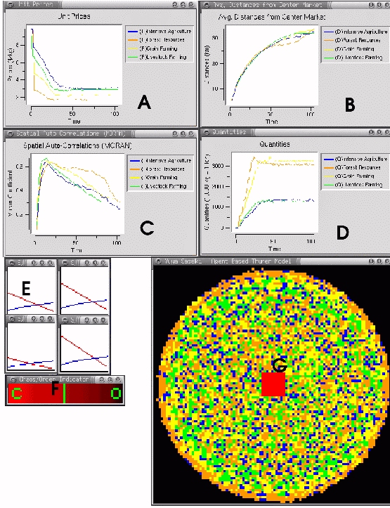
Figure 8. Graphical interface to agent-based model. A: Unit price for each agricultural product (x: time y: price) B: Average distance of agricultural type from city (x: time y: distance) C: Spatial autocorrelation of each agricultural type (x: time y: autocorrelation) D: Total quantity produced of each crop (x: time y: amount) E: Supply and demand graphs for each crop F: Chaos/Order graph G: Spatial representation of model

3.8

An additional property of the simulation turned out to be crucial in the appearance of von Thünen's rings, which can best be described as a variant of Langton's Lambda parameter (Langton 1991), a parameter that measures how close a system's behavior is to the boundary between chaos and order. Here we called a system completely chaotic if all the economic agents change professions at every time step, and completely ordered if no agents do so. If the simulation became completely chaotic, then no patterns would ever arise, and if the simulation became completely ordered, it would remain in a fixed pattern indefinitely. A graphic widget was created that would track the ratio of agents who changed professions (became farmers or city dwellers) to those who did not change (figure 8F). If a simulation run resulted in this graph going to either extreme, it was terminated and new input parameters tried.

3.9

Multiple iterations of this process led us to settle on the values in table 3. With those initial parameters a simulation run with both supply curves for the various agricultural products and radius of the isolated state remaining fairly constant and stable was achieved, which will be described in section 4. Observations about requirements of the initial parameters, with examples of model behavior under deviation from the initial parameters will follow in section 5.

Model Behavior

Typical Run

4.1

In each run, the model is initiated with no agricultural fields, and all agents occupying a city (number of city cells) at the center of the world (figure 9A). With no agricultural fields and no agricultural production whatsoever, the supply curves for all agricultural types are at 0 and opportunities for agents to produce all agricultural products is extremely high at that moment. This creates a boom for all agricultural types, and precipitates a mad land rush as agents settle the surrounding areas and set up production. This land rush lasts for about 100 time steps, at which time a radius is established that increases only gradually throughout the remainder of the run (figure 9C). At this point, there is no discernible pattern within the perimeter; however, there is still much movement of economic agents as they are affecting and being affected by the economic forces of the world in which they live.

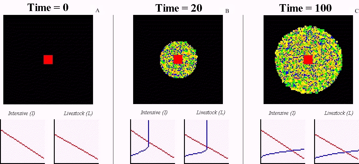
Figure 9. Simulation results for first 100 time steps

4.2

After 1000 time steps (figure 10A), there is still no discernible pattern within the perimeter of the state, though the boundary has grown slightly. After 3000 time steps (figure 10B), one can just begin to see a discernible aggregation of different agricultural types into concentric rings, and by 15,000 time steps (figure 10C) the patterns are well established and remain so indefinitely, at least until 500,000 time steps. At this point lock-in has occurred. The spatial pattern at that point conforms to the pattern in figure 7B.

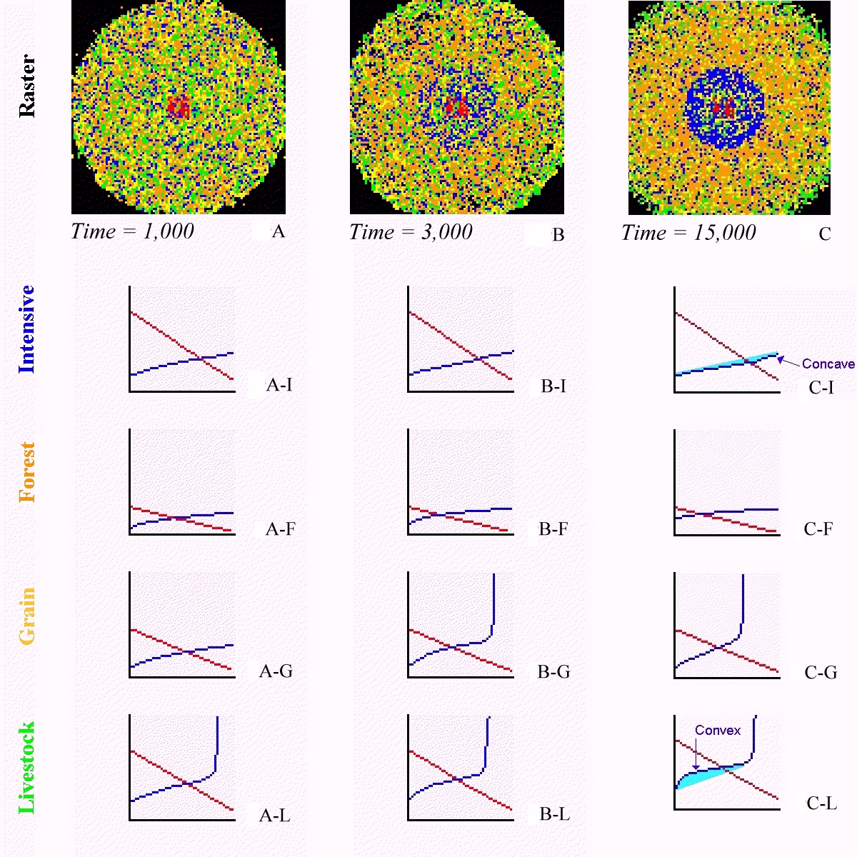
Figure 10. Simulation results from 1000 to 15,000 time steps

4.3

Lock-in is evidenced not only by the concentric rings in the market, but can be seen in the supply curves for each crop, whose derivative would show a skewed distribution on the price axis. The agricultural types associated with a weak F1 and strong F2, such as livestock farming (L), show a characteristic convex shape in the supply curve (figure 10C-L), which seems to conform to the graph in figure 3. Intensive agriculture (I), however, shows a concave shape in its supply curve (figure 10C-I), and seems to agree with the graph in figure 5. Each of these supply curves shift either upward or downward over time in a way that is also consistent with predictions in section 2.

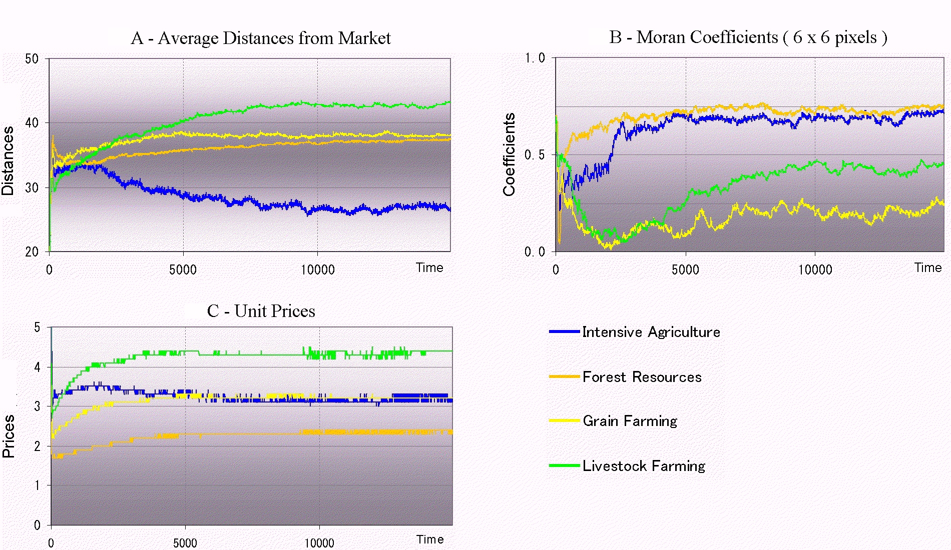
Figure 11. Time series of spatial and market trends for a single simulation run of 15,000 steps

4.4

Figure 11 shows a time series graph of three global properties of the simulation over a typical run (equivalent to the output graphs in figure 8A, B, and C). One can see that equilibrium price of each crop stabilizes relatively quickly, within 3000 time steps (figure 11C), and remains constant throughout the remainder of the run. Concurrent with this price stabilization is a preliminary separation of the average distances of crop types from the market (figure 11A), and a clear grouping (positive autocorrelation) of forest resources and later intensive agriculture (figure 11B). Notice that this accompanies only a faintly detectable spatial pattern (figure 10B).

4.5

As the simulation progresses, there is a slight but noticeable increase in separation of the average distances of some crops (figure 11A); intensive agriculture moves noticeably closer to market, while grain and forest resources merge towards the same average distance. However, there is much more land dedicated to forest resources; in figure 11B one can see that forest resources has a high positive autocorrelation while grain farming is close to zero. This is indicative of the fact that there is so much more land dedicated to forest resources, with grain farming inhabiting intermediate patches within the forest ring (visible in figure 10C). While grain farming commands a higher price (figure 11C) and higher demand (figure 10C-F, C-G), the market only supports this relatively small number of fields dedicated to its production. Livestock shows a somewhat greater distance in figure 11A, as it occupies the outer periphery of the area; the outer periphery becomes increasingly (but slowly) dedicated to livestock farming as the simulation progresses (figure 11B and 10B, C).

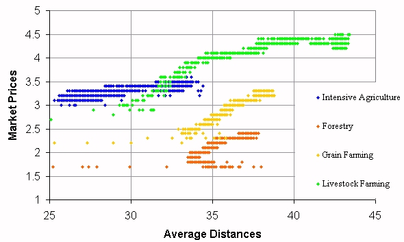
Figure 12. Correlation between average distance to market and unit price of crops

4.6

When the prices of the crops are compared to distance from the market for each individual producer after 15,000 time steps (figure 12), the segregation of crop types is also clearly visible. Also visible in this view is a clear correlation between distance from market and price. All four crop types yielded a positive correlation coefficient, with a confidence of dependency of virtually 100% (table 5).

Table 5: Correlations of crop prices with distance to markets for 15,000 agents after 15,000 time steps
	Coefficient	t	Coeff. Dependency
I	.47	65.21	100%
F	.70	120.04	100%
G	.70	120.04	100%
L	.79	157.80	100%

By time step 15,000, lock-in has occurred and there is no appreciable change in the state of the simulation after that, at least for 500,000 time steps (the longest that the simulation was run, about two week's computing time on our fastest available machine).

Experimental Runs and Observations

4.7

To understand the nature of this sort of model (called hypothetico-deductive characteristics in Nagel 1961), multiple runs with varying input parameters are needed. Multiple runs of the model were conducted with slight variations in area, productivity, and perishability of each agriculture type, and for average and standard deviation of city income. The values of the varying parameters of area, productivity, and perishability in each run were drawn from a normal distribution for each parameter tested, with a mean of the value presented in table 3. All other parameters were held constant, at the values presented in table 3. While this effort falls short of a formal sensitivity analysis, it allows for some preliminary observations to be made about the behavior of the model, and gives insight as to what aspects are most important to test in a more formal way. A more formal sensitivity analysis is currently being conducted by the authors.

4.8

Experimental runs were executed for 125 times with varying parameters, each with 10,000 time steps. While there were a variety of outcomes in the model runs, we observed some generalizations in model behavior that we categorized in the following way:

• category 1: "strong rings with expected spatial order"
  the average distances of lands for the four agriculture types from city center are ordered as proposed by von Thunen.
• category 2: "weak rings with expected spatial order"
  at most one pair of agriculture types are located at almost identical average distance from city center where the threshold value for the difference is half a cell size.
• category 3: "rings with at least one pair of land types swapped"
  at least one pair of agriculture types are located in different order from those predicted by von Thunen's rings, with the difference of the average distances from city center is greater than half a cell size.
• category 4: "static outcome"
  the failure of the model in that the little flow of population between city and agriculture industry makes the diameter of the state very small. This category is defined as at least one agriculture type has the average distance from city center less than twenty cell sizes.

4.9

As mentioned before, while the actual values for such parameters as productivity, demand, and perishability for each agriculture matter little to the model behavior, the relative values are crucial. In this preliminary exploration, average and standard deviation of city income seem to be the most important parameters to which the model outcome is sensitive. Table 6 shows the average coefficient of variation of city income for each model outcome category, and figure 13 shows the actual distribution of average and standard deviation of city income.

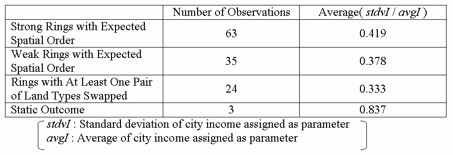
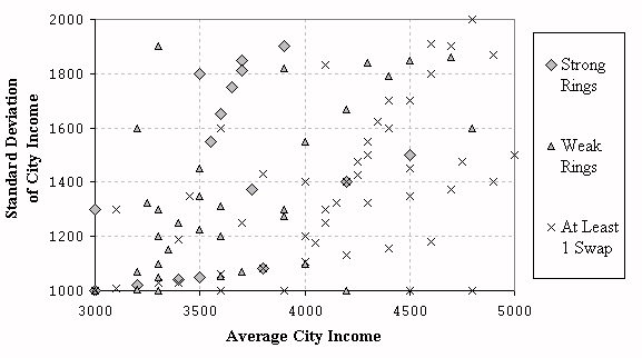
Table 6. Number of observations and average coefficient of variation of city income for each output category

Figure 13. The plot of output categories over standard deviation and average city income

4.10

The values in Table 6 indicate that greater standard deviation of city income relative to average city income tends to generate von Thunen rings, but too large one pushes the model to static behavior. The actual values for city income does not matter, since whatever value is given there will elicit a correction by causing market demand to be shifted outward. While this is not strictly pure inflation, it has a similar effect in our model. The importance of standard deviation of city income may be explained by its effect on the flow of people between city and agriculture jobs. The greater standard deviation, the greater the chance of dissatisfied city dwellers starting jobs in agriculture, with relatively wealthy city dwelling counterparts remaining in the city, satisfied to pay higher prices for agricultural products. This would give further incentive to poor city dwellers to start agriculture industry. This gives a frequent and flexible exchange of people between city and agriculture fields generating a greater probability of emergent optimization, since bottom-up trial and error actions are the sole drivers of this model. In this world, no global information given directly to agents beyond generalized price information in the inspiration cards. Table 6 also indicates that excessive coefficients of variation in city income causes too flexible of population exchanges, with most agents ending up being rich city dwellers.

4.11

Some validation of the importance of the coefficient of variation of city income is seen through an analysis of variance (ANOVA) testing a null hypothesis that the coefficient of variation of city income is not unique for each output category. Omitting the "static output" category, the summary in table 7 allows us to easily reject the null hypothesis; differences in the coefficient of variation of city income are indeed associated with different model outcomes.

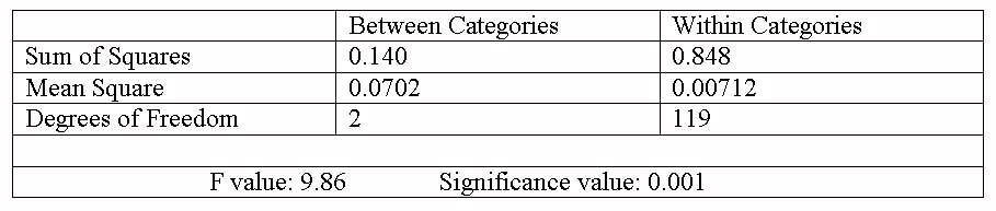
Table 7. ANOVA table

Conclusion, Discussion, and Future Work

5.1

In the model runs described in section 4, an optimal global solution emerged (formation of von Thünen's rings) without any systematic optimization functions at the system level. In accepted theory, it is assumed that individuals who participate in an economic system have perfect information and are rational decision makers with relatively complete information about their world, and can maximize their well-being simply by "adjusting their input variables". More recent theory emphasizes optimization of a whole system as something that emerges from simple agents acting on local criteria. In this case, von Thünen's rings emerged through collective actions of the agents. This ring-like structure is thought by many to be the most efficient spatial pattern for an isolated state.

5.2

In the context of this model, the emergence of macro structure from micro-behaviors should not really be a surprise. In reality, the role of agents' micro-behaviors in dealing with heterogeneous land cost leading to the emergence of von Thünen's rings has recently been explored and explained by the extended theories about long-term supply and Ricardian rent with spatial and/or land considerations. However, what we employed for this model are the discrete elements that work behind the spatial constraints, whereas the continuous nature is the essential assumption in the theoretical approach. The agents in our model are assumed to be reflex agents. Given these characteristics, plus the homogeneities of the lands, space alone turned out to be at least as important as land cost and critical mass of terms of transportation networks. The best analogy will be the principle of swarm intelligence, in which a group of simple agents (such as ants) collectively end up with some optimal solution as a result of spatial and temporal complexities. Of course, humans are more complex and intelligent beings, and not such "simple" agents. Yet, by reducing their motivations as those of simple agents, the complex interactions with space give us sufficient power for optimization. These conclusions are still preliminary, and will require a formal sensitivity analysis of the model to allow us to state them with greater confidence.

5.3

While this model helps us in understanding some of the theoretical connections between individual actions and global behavior in a simplified system, ultimate utility of this model may be in real world applications. As we commented previously, ABMs are not suited for real world prediction. They are best used for understanding how processes interplay in a system; insights into the fundamental driving mechanism of positive feedbacks and lock-in agree with some accepted theory, and seem to be valid. Though von Thünen's rings are seldom seen today primarily due to the changes in environmental variables (technological advances and the decrease in human demands for necessities, etc.), and the spatial consideration for the lock-in pattern are still apparently valid. A simple real-world application may be done by adjusting input parameters in Table 3 to the local situations of the regions of interest. More meaningful application would come through integrating this model with known information in an area, including landscape information through spatial databases (GIS) and socioeconomic data from public census or other survey information. While we have experimented with the model in a simple homogeneous landscape for analytical purposes, the use of GIS raster data or classified satellite images could serve as a more realistic stage for the agents' interactions.

References

ANTONA M, Bommel P, Fran c B, and Le Page C (2002) Interactions and organization in ecosystem management: The use of multi-agent systems to simulate incentive environmental policies. Lecture Notes in Agent-Based Simulation, 3. Passau, Germany April 7-9, 2002.

ARTHUR B W (1987) Path-dependent processes and the emergence of macrostructure. European Journal of Operational Research, 30. pp. 294-303.

ARTHUR B W (1990) Positive Feedbacks in the Economy. Scientific American, Feburary 1990. pp. 92-99.

AXELROD R (1997) "Advancing the art of simulation in the social sciences". In R. Conte, R. Hegselmann and P. Terna (Eds) Simulating Social Phenomena. Springer

AXELROD R M (1984) The Evolution of Cooperation. Basic Books, New York.

BLOCK D and DuPuis M E (2001) Making the country work for the city: von Thünen's ideas in geography. American Journal of Economics & Sociology, 60(1). pp. 79-99.

BOUSQUET F and Gautier D (1998) Comparasion de deux approches de modélisation des dynamiques spatiales par simulation multiagents: les approches spatiales et acteurs. CyberGéo, 89.

BOX P W (2002), "Spatial units as agents: Making the landscape an equal player in agent-based simulations". In Gimblett H R (Ed.), Integrating Geographic Information Systems and Agent-Based Modeling Techniques for Understanding Social and Ecological Processes, Life Sciences, Oxford. Oxford University Press. pp. 59-82.

CHISHOLM M (1981) Rural Settlement and Land Use: An Essay in Location. Nethuen Drama.

CLARKE K C, Hoppen S, and Gaydos L (1997) A self-modifying cellular automaton model of historical urbanization in the San Francisco Bay area. Environment and Planning B: Planning and Design, 24. pp. 247-261.

DEADMAN P J (1999) Modeling individual behavior and group performance in an intelligent agent-based simulation of the tragedy of the commons. Journal of Environmental Management, 56. pp. 159-172.

DEAN J S, Gummerman G J, Epstein J M, Axtell R L, Swedland A C, Parker M T, and McCarroll S (2000), "Understanding Anasazi culture change through agent-based modeling". In Kohler T A and Gumerman G J (Eds.), Dynamics in Human and Primate Societies: Agent-Based Modeling of Social and Spatial Processes, Studies in the Sciences of Complexity. Santa Fe Institute, Oxford University Press. pp. 179-206.

HOLLAND J H (1995) Hidden Order: How Adaptation Builds Complexity. Perseus Books, Cambridge, MA.

KOHLER T, Kresl J, Van West C, Carr E, and Wishusen R H (2000), "Be there then; a modeling approach to settlement determinants and spatial efficiency among late ancestral pueblo populations of the Mesa Verde region, U.S. southwest". In Kohler T A and Gumerman G J (Eds.), Dynamics in Human and Primate Societies: Agent-Based Modeling of Social and Spatial Processes, Studies in the Sciences of Complexity. Santa Fe Institute, Oxford University Press. pp. 145-178.

KOHLER T and Van West C (1996) "The calculus of self interest in the development of cooperation: Sociopolitical development and risk among the northern Anasazi". In Tainter J A and Tainter B B (Eds.), Evolving Complexity and Environment: Risk in the Prehistoric Southwest, volume XXVI of Santa Fe Institute Studies in the Sciences of Complexity, Reading, MA. Addison-Wesley. pp. 171-198.

LANGTON C G (1991), "Computation at the edge of chaos: Phase transitions and emergent computation". In S. Forrest. Emergent computation : Self-organizing , collective, and cooperative behavior in natural and artificial computing networks. Cambridge MA: MIT Press, pp.12 - 37.

LIM K, Deadman P, Moran E, Brondizio E, and McCracken E (2002), "Agent-based simulations of household decision making and land use change near Altamira, Brazil". In Gimblett H R (Ed.), Integrating Geographic Information Systems and Agent-Based Modeling Techniques for Understanding Social and Ecological Processes, Life Sciences, Oxford. Oxford University Press. pp. 277-310.

MANSON S M (2000), "Agent-based dynamic spatial simulation of land-use/cover change in the Yucatán peninsula, Mexico". In 4th International Conference on Integrating GIS and Environmental Modeling (GIS/EM4): Problems, Prospects and Research Needs, Banff, Alberta, Canada. NCGIA. Sept 2-8, 2000.

MINAR N, Burkhart R, Langton C, and Askenazi M (1996) The Swarm simulation system: A toolkit for building multi-agent simulations. Santa Fe Institute Working Paper 96-06-042.

NAGEL, E. (1961) The Structure of Science: Problems in the Logic of Scientific Explanations. Harcourt, Brace, and World, NY.

OTTER H S, van der Veen A, and de Vriend H J (2001) ABLOoM: Location behaviour, spatial patterns, and agent-based modeling. Journal of Artificial Societies and Social Simulation, 4(4). <https://www.jasss.org/4/4/2.html>.

PARKER D C (2000) Edge-Effect Externalities: Theoretical and Empirical Implications of Spatial Heterogeneity. PhD thesis, University of California, Davis, CA.

PEET J R (1969) The spatial expansion of commercial agriculture in the nineteenth century: a von Thünen interpretation. Economic Geography, 45. pp. 283-301.

TORRENS P M and O'Sullivan D (2001) Cellular automata and urban simulation: Where do we go from here? Environment and Planning: B, 28. pp.163-168.

VON THÜNEN J H (1826) Die isolierte Staat in Beziehung auf Landwirtshaft und Nationalökonomie. Pergamon Press, New York. English translation by Wartenberg C M in 1966, P.G. Hall, editor.

WARTENBERG C M (1966) The Isolated State: an English Edition of Der isolierte Staat. Pergamon Press.

Return to Contents of this issue

© Copyright Journal of Artificial Societies and Social Simulation, [2003]