Massimo Sapienza (2003)
Do Real Options perform better than Net Present Value? Testing in an artificial financial market
Journal of Artificial Societies and Social Simulation
vol. 6, no. 3
To cite articles published in the Journal of Artificial Societies and Social Simulation, please reference the above information and include paragraph numbers if necessary
<https://www.jasss.org/6/3/4.html>
Received: 10-Nov-2002 Accepted: 5-Apr-2003 Published: 30-Jun-2003
 Abstract
|
where V(dt) is the NPV value of the project already in place and F(dt) is the value of the growth option that the firm can exercise when the cash flow is above its trigger value d*.
 .
.
|
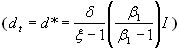
with  is the cash flow's average rate of growth.
  is the scale multiplicative factor of the cash flow (under our assumptions equal to the dividend). It indicates how big the impact of new investments on cash flow will be when the expansion option is exercised. I is the exercise cost of the option, the value of the investments required to expand the scale. We assume and I to be common knowledge.
 and making investments of amount I or to keep the expansion optino F(dt) alive and so obtaining the dividend dt from the project which is already implemented.
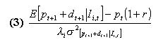
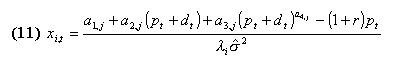
 from the standard maximization problem we get the investor's i demand function for the risky asset at time t:
|
where  is the agent's degree of relative risk aversion. The risky asset's demand is a function of the expected excess return E[ pt+1+dt+1] which the trader can obtain by investing in this asset rather than the riskless one.
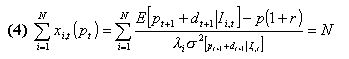
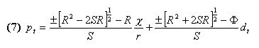
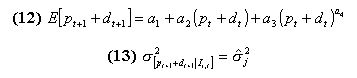
The model is closed by determining the clearing price p by setting the demand equal to the supply (i.e.. by assuming one share supplied per agent):
is the agent's degree of relative risk aversion. The risky asset's demand is a function of the expected excess return E[ pt+1+dt+1] which the trader can obtain by investing in this asset rather than the riskless one.
The model is closed by determining the clearing price p by setting the demand equal to the supply (i.e.. by assuming one share supplied per agent):
|
|
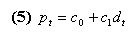
This assumption is perfectly in line with an NPV valuation process of firms.
 and when dividends are distributed according to a geometric Brownian motion.
|
|
 . The conditions for the existence of a linear rational expectations equilibrium when the dividends process is a geometric Brownian motion appears extremely restrictive given the values of stock prices variances and the investors' risk aversion generally assumed in the ACF[11]. Nevertheless it seems reasonable to investigate whether a non-linear specification of the relationship between price and dividend could be more useful in finding an REE for the case of dividends distributed according to a geometric Brownian motion. Real Options provide a fundamentalist explanation of this non-linear specification. We will illustrate our results in the next sub-sub-section.
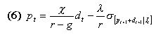
 , the price of the risky asset is a non-linear function of the current dividend dt.
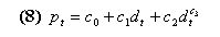
|
 for the coefficients c2 and c3. We are fully aware of the loss of generality induced in our results by this ''guessing'' approach, but we should not, on the other hand, forget our research goal, which is to test whether the ROV technique is a superior tool for valuation in financial markets. Our behavioral restriction is very important if someone wishes to establish if, in general, a vector c0, c1, c2, c3 that constitutes an REE exists, but it is not so important if we limit ourselves our study to NPV and ROV based equilibria.
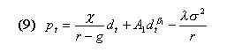
|
|
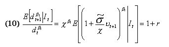
 and should be equal to 1 plus the risk less rate r , the expansion option regime, in order to be a rational expectations equilibrium. This statement is, in some way, similar to the bubble growth condition of Froot and Obstfeld. This ''unstable'' condition may help us to explain phenomena like the recent New Economy boom and burst. An equilibrium with agents who incorporate the growth option value of firms is ''fragile'', as we noticed above. The collapse of high tech firms' valuation may be explained in terms of a ''jump out'' of the ROV based REE due to some disturbances in the expectations on .
| Agent | Rationality |
| Random | None |
| Market Imitating | Imitation |
| Stop Loss | Rule of thum |
| Forecasting | ANN based forecasting |
| Cross Targets | Cognitive abilities |
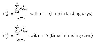
 and
and  transmitted by the detectors to the classifiers systems and used to calculate the option value are computed by using an historical measure of these two volatilities[15].
|
 .
.
 formed by the classifiers system, the agent can calculate the desired risky asset holdings according to (5.7), compare it with its endowment and submit to the book an appropriate order:
|
|
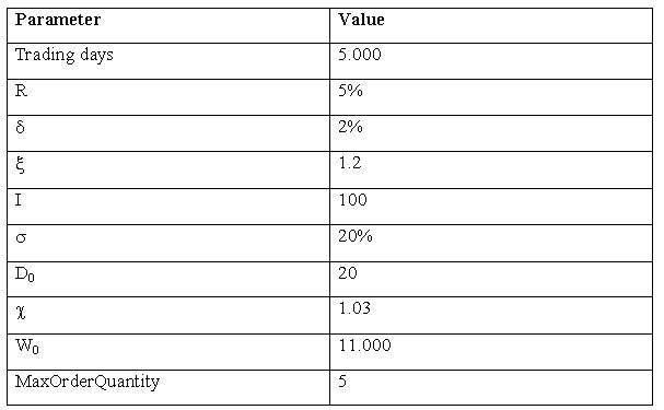
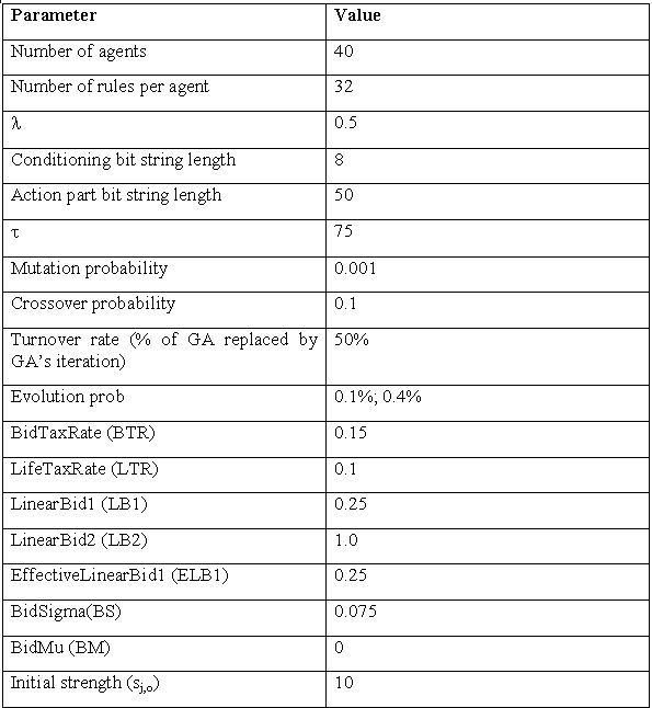
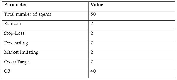
| Table 3. Main simulation parameters |
 |

|
 and of the starting 32 rules of each classifiers system are set to random values distributed uniformly through the REE equilibrium forecast values. The first 32 rules constitute some sort of ''common knowledge.'' These 32 rules are set-up by using some kind of ''standard rationality'', which links the conditioning and the actioning part of each rule. For instance if the conditioning part is not imposing any requirement on ROV and Incorrect ROV bits then the value of the non-linear option based parameters are set as equal to zero. Such coherence is not present a priori in the rules generated by the classifiers system, because we would like to allow agents to have the incoherencies that are frequently observed among investors.
|
| Table 4. Classifier system's parameters |
|
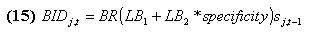
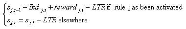
where specificity is the relative specificity of the rule: the ratio between the number of # in both the action and the conditioning part and the length of the rule. The purpose of this cost is to make sure that each bit is actually serving a useful purpose in terms of a forecasting rule; sj,t-1 is the strength of rules j at time t-1, W is a random real number between 0 and 1. Bidj,t is the amount the auction's winner actually has to pay.
 |
|
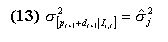
 determines the horizon length that the agent considers relevant for forecasting purposes. If =1, then the rules only use the last period forecast error. If the agents use all past data then they would be making the implicit assumption that the world they live in is in a stationary state. The value of is critical and we are still waiting for a theory that will allow us to endogenize that parameter. We will use the value used by Arthur et al. (1997) and by Le Baron et al. (1999) of 75 in our simulation. The reward is then calculated by comparing the accuracy of the activated rule, with the mean accuracy of the previous activated rules. If the accuracy v2j,t is below the average, the reward is equal to 1; if v2j,t is equal to the average, the reward is 0; and finally if v2j,t is greater than the average, the reward is equal to 1.
|
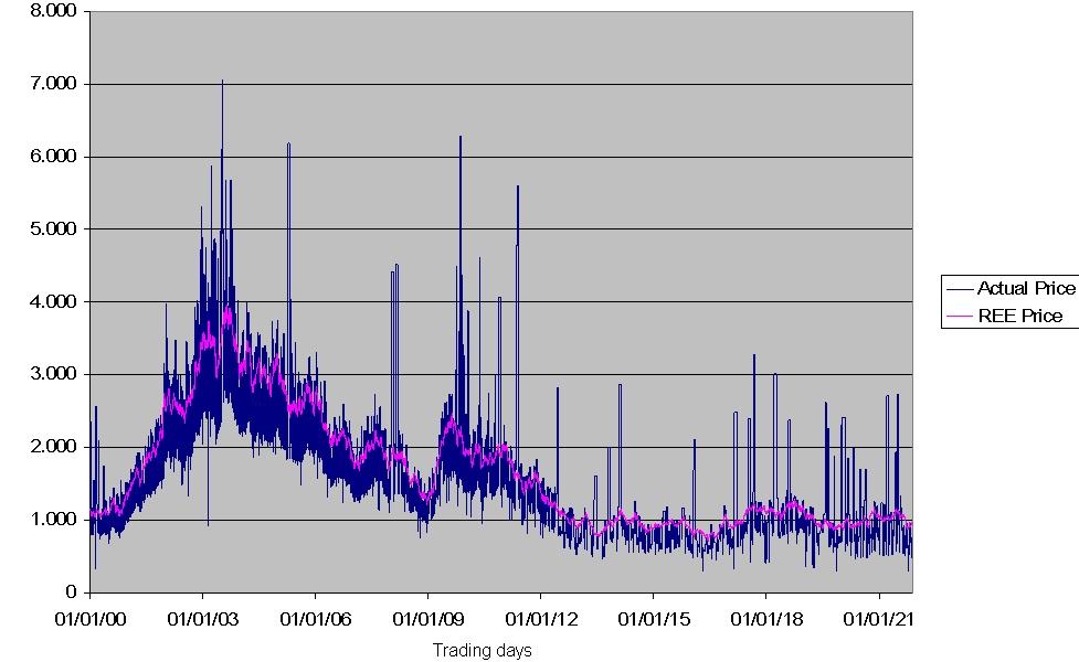
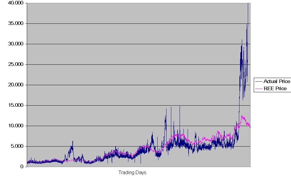
| Figure 1. Actual and REE prices in the HOCA Slow learning case |
|
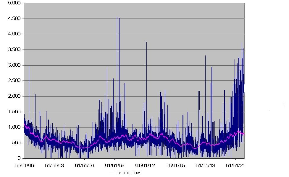
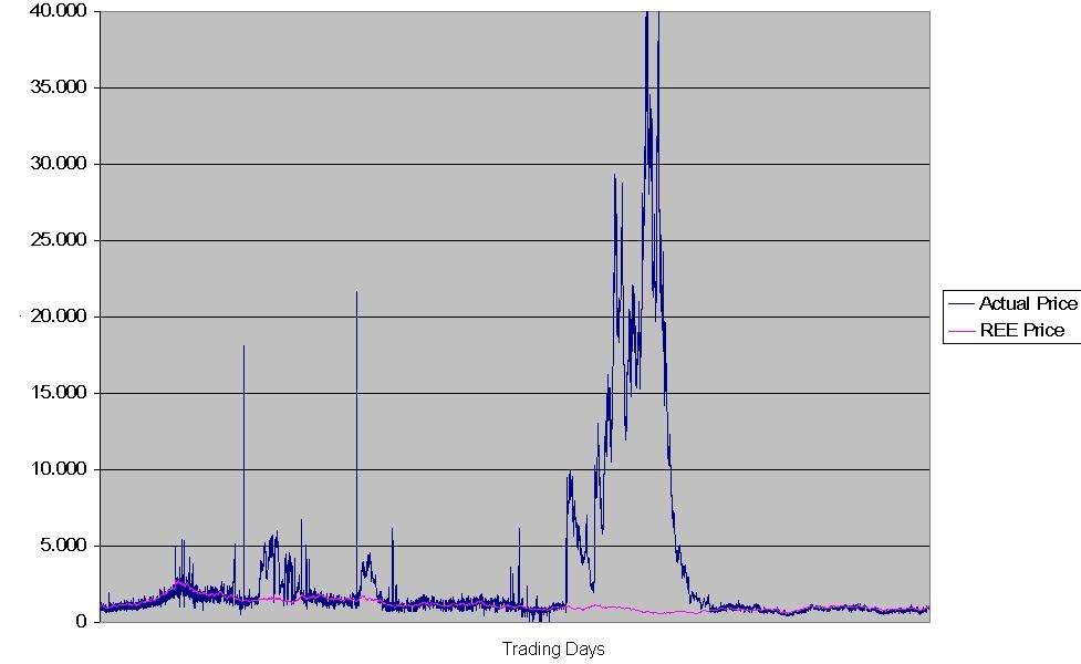
| Figure 2. Actual and REE prices in the HOCA fast learning case |
|
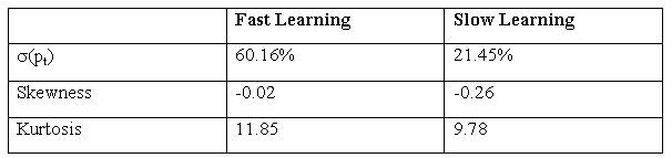
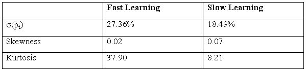
| Table 5. Data on prices - HOCA |
|
|
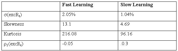
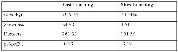
| Table 6. Data on returns - HOCA |
|
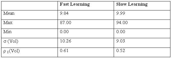
| Table 7. Trading volume - HOCA |
|
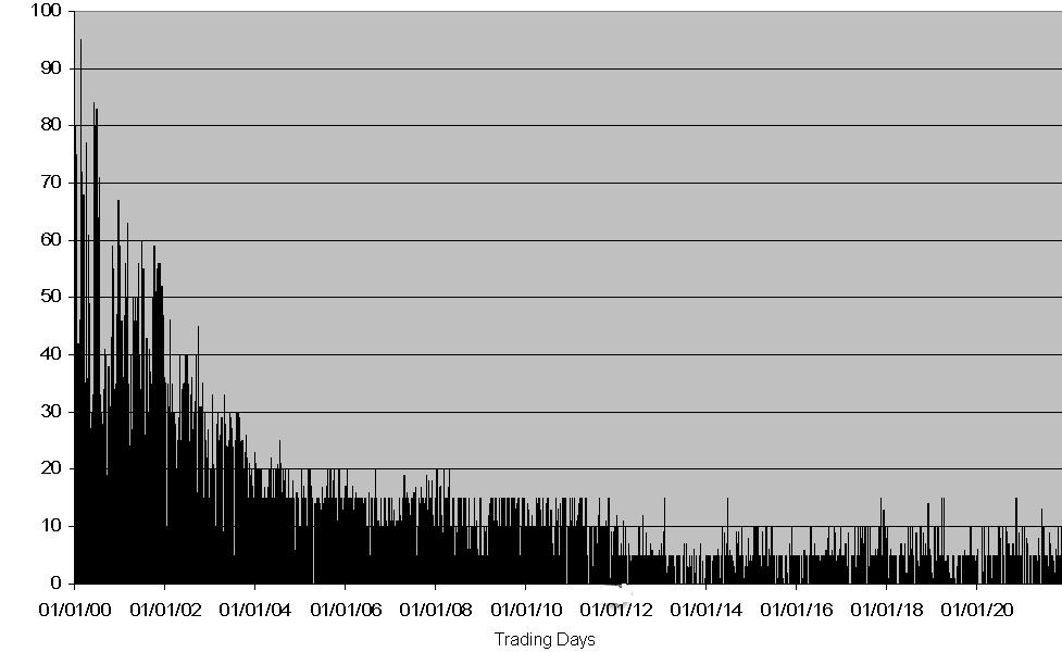
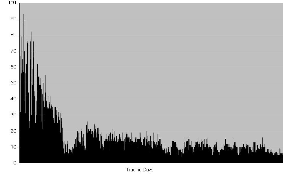
| Figure 3. Volume in the HOCA slow learning case |
|
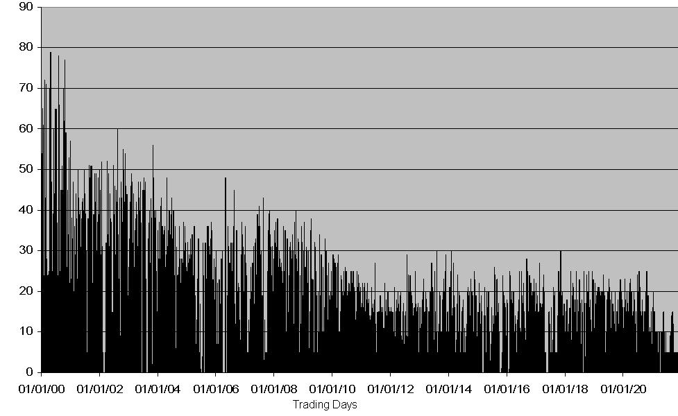
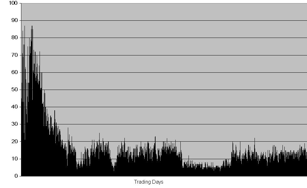
| Figure 4. Volume in the HOCA fast learning case |
|
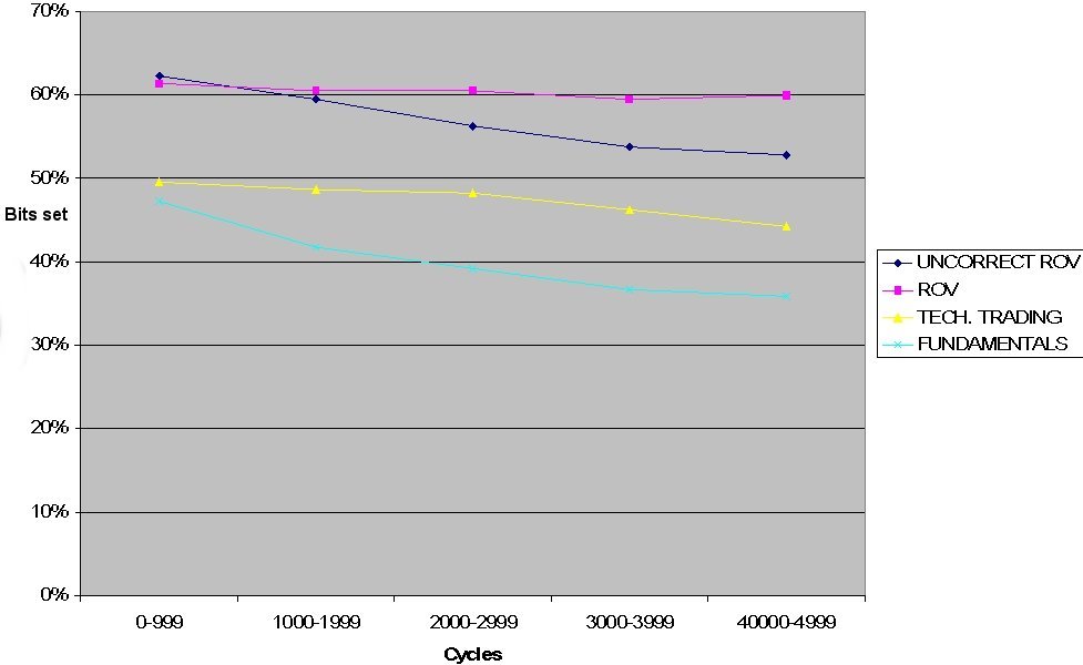
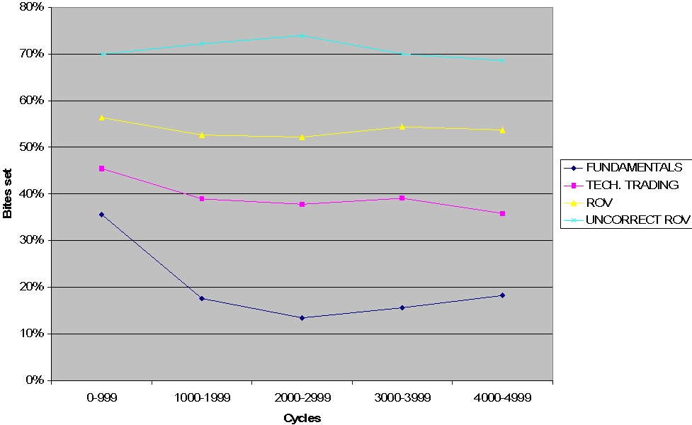
| Figure 5. Percentages of the conditioning part's bit set - HOCA slow learning case |
|
| Table 8 |
|
| Table 9. Da on prices-HECA |
|
| Table 10. Da on returns-HECA |
|
| Figure 6. Volume in then HECA slow learning case |
|
| Figure 7. Volume in then HECA fast learning case |
|
|
| Table 11. Trading volume-HECA |
|
| Figure 8. Actual and REE prices in the HECA slow learning case |
|
| Figure 9. Actual and REE pices in the HECA fast learning case |
|
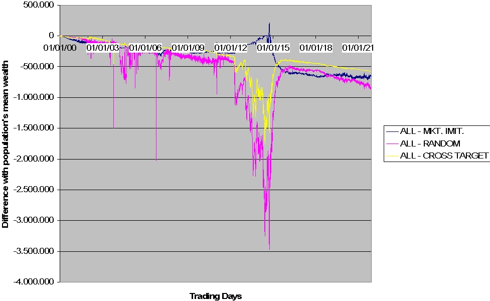
| Figure 10. CS agents performance |
|
| Figure 11. Well performing agents in the HECA fast learning case |
|
| Figure 12. Percentages of the conditioning part's bit set - HECA fast learning case |
2See among others: Arthur et al. (1997), Chen , Yeh (2001), Tay and Linn (2001), Terna (2001).
3See: Arifovic (1996), Arifovic (2000).
4See: Le Baron et al. (1999), Lawenz and Westerhoff (2000)
5Minar, Burkhart, Langton and Askenazi (1996) present the software. For a detailed user's guide see Johnson and Lancaster (1999). A tutorial by Stefansson is also contained in Luna and Stefansson (2000). Complete software documentation, source code and much other interesting material is available at: <http://www.swarm.org>.
6In the time frame of the model, dividends are payed every 30 cycles; Each cycle represents a trading day. Dividends are obviously distributed to traders proportionally to their holdings.
7In the version of SUM presented by Terna (2001) any kind of fundamentals is totally absent. The risky asset does not entitle the agent to earn any dividend, and consequently it's value is purely bubbly. The Santa Fe Stock market assumes that the dividend process is a mean reverting process. No assumptions are made about the relationship between the firm's cash flow and the dividends payed
8We could also relax this assumption by considering the firm as a portfolio of different projects, but for the sake of simplicity we prefer to maintain this mono-project scheme.
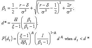
9By calculating the expansion option's value we obtain the following results:
10See for instance Arthur et al. (1997), Le Baron et al. (1999), Tay and Linn (2001), Chen and Yeh (2001).
11With σ=20% and λ=0.5 we would need a risk less interest rate greater than 40% to obtain a real value for the REE price. However we should point out that there is practically no evidence available to calibrate the parameter λ. The value of 0.5 has been practically just assumed. With λ in the range [ 0.01,0.1] we obtain values of the interest rate highly similar to those actually observed.
12 In the following exposition 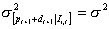 is instead the standard deviation of the dividends' process, the geometric Brownian motion.
13Here is a strong difference with respect to the Santa Fe stock exchange market. In that context, agents are heterogenous in their learning history and in their knowledge but they share the same learning mechanisms. In that context all the agents have rationality empowered by a classifiers system.
14Finally we have to add that our analysis is restricted to just one example of trading mechanism present in the financial markets. A different analysis on the impact of alternative trading schemes is left for future research.
15More specifically in the simulation the following historical estimators for volatility are employed:
16As an exemplification let consider the following conditions: [1 # # # # # # # # # # 1 1 # #] recognizes the states where the current price times the interest rate divided by the current dividend is below a quarter AND the dividend estimated volatility is greater than 30%.
17The simulation code is available on-line at: <http://web.tiscali.it/msapienza/acepaper.htm>
18To provide Monte Carlo-like evidence of the stochastic robustness of the results, running a sample of simulations under different random seeds would be desirable. Unfortunately this interesting exercise has not been done systematically. It is our aim to complete this research work in the near future. The 4 simulations illustrated in the text are based on different random seeds to allow some kind of statistical heterogeneity. In any event, two main elements avoid any inconsistency caused by the "real randomness" of the four simulations: the growth option continuous appearance mechanism which makes new options appear once the old one are exercised, and the initial calibration of the growth option which is "out-of-the money". These two elements make any slight difference in the dividend process almost irrelevant so as to determine which trading strategy is performing better.
19 In the original ASM (artificial stock market) configuration the initial rules' databases were composed by 100 rules per agent.
20This algorithm described in Goldberg (1989) is quite standard in classifiers systems applications. It avoids the eccessive determinism which would be caused by a selection process only based on fitness measures. ASM does not exploit the advantages of such a selection process and relies on a purely deterministic mechanism. We consider this point as a significant improvement of our model.
21 More than two years.
ARIFOVIC J. (2000). "Evolutionary dynamics of currency substitution", Journal of Economic Dynamics and Control, vol. 25, n. 3-4, pp. 395-417.
ARTHUR W.B., HOLLAND J., LE BARON B., PALMER R., TAYLER P. (1997), ''Asset pricing under endogenous expectations in an artificial stock market'', in Arthur W.B., Durlauf S., Lane D. (eds.), ''The economy as an evolving complex system II'', Santa Fe institute in the science of complexity, vol. XXVII, Addison-Wesley, Reading, pp. 15-44.
AXTELL R. (2000), ''Why agents? On the varied motivation for agent computing in the social sciences'', Center on social and economic dynamics working paper n. 17, <http://ww.brookings.edu/es/-dynamics/papers/agents/agents.htm>.
BLUME L., EASLEY D. (1982), ''Learning to be rational'', Journal of Economic Theory, n. 26, pp. 340-51.
BLUME L., EASLEY D. (1992), ''Evolution and market behavior'', Journal of Economic Theory, n. 58, pp. 9-40.
BRAY M. (1982), ''Learning, estimation and the stability of rational expectations'', Journal of Economic Theory, n. 26, pp.318-339.
CHEN S, YEH C. (2001), ''Evolving traders and the business school with genetic programming: a new architecture of the agent based artificial stock market'' Journal of Economic Dynamics and Control, vol. 53, n. 3-4, pp. 363-93.
FERRARIS G. (1999), ''Algoritmi genetici e classifiers systems in Swarm: due pacchetti per la realizzazione di modelli, due applicazioni economiche ed un. formichiere affamato'', mimeo, Turin paper presented at IRES conference ''Simulare con Agenti per l'analisi socieconomica'' 28th October 1999.
FROOT K. A., OBSTFELD M. (1991), ''Intrinsic bubbles: the case of stock prices'', American Economic Review, vol. 81, n. 5, pp. 1189-1214.
GODE D.K., SUNDERS S. (1993), "Allocative efficiency of markets with zero intelligence (ZI) traders: market as a partial substitute for individual rationality", Journal of Political Economy, Vol 101, pp. 119-37.
GOLDBERG D. (1989), ''Genetic algorithms in search, optimization & machine learning'', New York, Addison-Wesley.
JOHNSON P., LANCASTER A. (1999), ''Swarm user guide'', mimeo.
LAWRENZ C., WESTERHOFF F. (2000), "Explaining exchange rate volatility with a genetic algorithm" mimeo, paper presented at VI International conference of the society of Computational Economics on Computing in Economics and Finance, July 6-8, Universitat Pompeu Fabre, Barcelona, Spain.
LE BARON B. (2000), ''Agent based computational finance: suggested readings and early research'', Journal of Economic Dynamics and Control, vol. 24, n. 5-7, pp. 679-702.
LE BARON B, ARTHUR W. B., PALMER R. (1999), ''Time series properties of an artificial stock market'', Journal of Economic Dynamics and Control, vol. 23, n. 9-10, pp. 1487-1516.
LUNA F., STEFANSSON B. (2000), ''Economic simulation with Swarm: Agent based modelling and object oriented programming'', Dordrecht and London, Kluwer Academic Press.
Luna F., Perrone A. (2001), ''Agent based methods in Economics and Finance: simulations in Swarm'', Dordrecht and London, Kluwer Academic Press MINAR N., BURKHART R., LANGTON C., ASKENAZI M. (1996), ''The SWARM simulation system: a tool-kit for building multi-agent simulations'', working paper Santa Fe Institute.
TAY N., LINN S. (2001), ''Fuzzy inductive reasoning, expectation formation and the behavior of security prices'', Journal of Economic Dynamics and Control, vol. 25, n. 3-4, pp. 321-361.
TERNA P. (2001), ''Cognitive agents behaving in a simple stock market structure'', in F. Luna and A. Perrone (eds.), ''Agent based methods in Economics and Finance: simulations in Swarm'', Dordrecht and London, Kluwer Academic Press.
 Return to Contents of this issue
© Copyright Journal of Artificial Societies and Social Simulation, [2003]