Hu Bin and Xia Gongcheng (2005)

Integrated Description and Qualitative Simulation Method for Group Behavior

Journal of Artificial Societies and Social Simulation vol. 8, no. 2
<https://www.jasss.org/8/2/1.html>

To cite articles published in the Journal of Artificial Societies and Social Simulation, reference the above information and include paragraph numbers if necessary

Received: 16-Mar-2004    Accepted: 28-Dec-2004    Published: 31-Mar-2005

Abstract

This paper presents a qualitative simulation method for analyzing employee group behavior by integrating QSIM (Qualitative SIMulation) with basic causal reasoning. A description method for complex interactions between environment, management policy and group behavior is designed. A qualitative simulation method including the simulation rules and a simulation engine is then proposed. The validation of the proposed method is tested, and an example is given of how this method can be applied to the development of management policy for the effective motivation of employees. Simulation results show that this method can be used to explain and predict changes in group behavior, and also to aid in decision making on employee group management.

Keywords:

Group behavior, Qualitative Simulation, QSIM, Causal Graph, Group Dynamics

Introduction

1.1

Quantitative simulation is utilized in scientific disciplines as a computer based tool of optimization, design and decision-support for systems. However, it is not widely accepted in the management field (Berends and Romme 1999). Most management systems (such as those in human resources) are used to manage people, and people are greatly affected by their environment. A quantitative model is not appropriate for the analysis of group dynamics and so is not generally used. However, having a virtual tool for experimentation and to aid in decision making involving a complex set of factors is desirable among enterprise managers.

1.2

Because of the complex and abstract nature of group dynamics, it is difficult to acquire accurate numerical information on which managers can base decisions. Most of the information acquired in this way is ambiguous, incomplete or qualitative in nature. Therefore most decisions are, in practice, not based on precise numerical information but on information that is empirical and/or qualitative. Human resource management is a good example of where this is very common.

1.3

For example, in the selection and recruitment of individuals for the key positions in an enterprise, there are usually several factors taken into consideration, such as disposition, personal history, etc. It is impossible for employers to make a precise and accurate numerical assessment of an individual based on this kind of information. These factors can not be quantified. What employers need is a qualitative method of evaluating each candidate.

1.4

The challenge is how to accurately determine who in a selection of candidates is best suited for the position in question. In virtual experiments using qualitative simulation, employers determine which candidate is the best suited to the position for which employers are hiring.

1.5

A quantitative approach to the development of strategies for motivating employees is also inappropriate. Accurate numerical information usually can not be obtained by evaluating employee attitudes and performance, i.e. group cohesion, company loyalty, etc., and the data can be obtained is not useful. Precise scores in this sort of assessment are impossible to interpret accurately and meaningfully. So a qualitative approach is necessary for this kind of evaluation.

1.6

Qualitative simulation is a better approach when choosing between strategies once they have been developed. Managers develop several possible alternative policies for employee motivation and then must determine which policy to select. A simulation is run on each alternative, and then a decision is made based on the simulation results. A quantitative simulation approach would not be possible. Therefore a qualitative simulation is what must be used.

1.7

In the qualitative simulation of physical systems there are generally two elements used to express qualitative value: "level" and "change of direction" (Kuipers 1994). The level scale includes three levels; "low", "moderate" and "high". The change of direction scale includes three directions; "decrease", "standard" or "increase" (expressed as "-", "0" and "+", respectively). For example, "Loyalty to Organization" can be expressed as being "high" and "+". This means that there is a high degree of loyalty among employees and that it is continuing to increase. When developing strategies for employee motivation, qualitative data as expressed above is far more useful than data that is precise and numerical.

1.8

In this paper, we propose a method of qualitative simulation for the assessment and prediction of employee group behavior. This method can serve as the foundation of qualitative simulation in the field of human resource management, where every system orients to the group rather than the individual. For example, in the recruitment and selection of managers, a simulation should not be run on the candidate as an individual, but rather on how the candidate is likely to affect the group that he or she would be managing. When considering a potential policy change for employee motivation, a simulation should not be run on the policy itself, but on the effect that the policy will have on employees and how it is likely to influence their behavior.

1.9

The organization of this paper is as follows. QSIM and causal reasoning are surveyed in paragraphs 1.10 to 1.22. Our method of integrating QSIM and causal reasoning is explained at 1.23. In Section 2, a description of variables, distinguished time points, landmark values and group behavior causality is given. In Section 3, the rules of this method are explained and a simulation engine is illustrated. The validity of this method is tested in Section 4 and its application is illustrated in Section 5. Conclusions and directions for future research are given in Section 6.

QSIM

1.10

Since QSIM (Qualitative SIMulation) was introduced (Kuipers 1986), it has been widely accepted for the study of physical systems (Kuipers 1993a; Kuipers 1993b; Clancy and Kuipers 1998).

1.11

There have been many improvements to the QSIM method (Platzner and Rinner 2000; Weld 1990; Shen and Leitch 1993). Platzner et al (1997) parallelized the complex functions of simulated objects in order to improve the performance of QSIM. Weld (1990) modified the quantity space of QSIM, so that the qualitative values of state variables can now have four possible orders of magnitude. Shen and Leitch (1993) combined Fuzzy sets with QSIM to make it more detailed and comprehensive.

1.12

QSIM provides a tool for the analysis and explanation of the behavior of physical systems, although it has also been used in biology (Guerrin and Dumas 2001). The QSIM method, as well as its results, is incomplete (Cem Say and Akyn 2003) and should therefore be used in combination with other methods.

1.13

In this paper we integrate the description method of QSIM with basic causal reasoning. To understand our approach, the description method of QSIM is given below.

1.14

QSIM consists of four components: qualitative state description, qualitative state constraints, transition rules and a simulation engine (Kuipers 1986; Kuipers 1994).

1.15

State variables are the components of a system. The qualitative value of a state variable is described as: QS(x_i, t_j) or QS(x_i, t_j, t_j+1) = <qval_i, qdir_i>, x_i ∈ X, i ∈ {1,2,...,n}, t_j or t_j+1 ∈ T, j or j+1 ∈ {0,1,2,...,m}, where X is the set of state variables and T is the set of distinguished time points at which the state of the system has the distinguished value. QS(x_i, t_j) and QS(x_i, t_j, t_j+1) represent the qualitative value of x_i at the time point t_j and in the time interval (t_j, t_j+1), respectively. qval_i is the level of QS, qdir_i is the change direction. They are specified as follows:

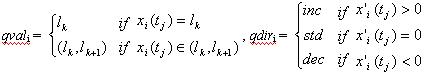
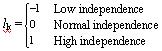
where l_k or l_k+1 ∈ L, k or k+1 ∈ {1,2,...,p}, L is the quantity space of the landmark values (the values of state variables at distinguished time points). inc, std and dec represent the change direction of x_i. inc means "increase", dec means "decrease" , and std means "standard" (no change).

1.16

For example, when describing the temperature change of a glass of water, there are at least two landmark values: 0⁰ C and 100⁰ C. Once the water has been boiled and removed from heat, the temperature change can be described as QS(water_temp, now) = <(0⁰C, 100⁰C), dec>.

1.17

For other components of QSIM, see Kuipers (1986 and 1994), which discuss the concepts, definitions and methods of QSIM in detail.

Causal reasoning

1.18

The Causal Reasoning Method is derived from the causality theory provided by Simon in 1950. Iwasaki and Simon (1986) used this method to analyze the behavior of physical systems. Iwasaki (1988) used it to build a system model consisting of both static and dynamic relations. Salvaneschi et al (1997) combined a qualitative causal framework with quantitative relations to support the modeling and simulation of a physical system.

1.19

The Causal Reasoning Method was developed by integrating mathematical methods (probability, the Markov assumption, etc.). Since 1980 some causal modeling methods (e.g. Bayesian networks and structural equation models) have emerged from converging work in statistics, philosophy and artificial intelligence (Glymour 2003). The theory of causal modeling is thoroughly studied in Pearl (2000). Pearl discusses information flow among the variables, validity of the proposed model, minimality and stability of the model, the effect of time on causality, etc.

1.20

The Causal Reasoning Method has been widely used in the field of economics. Lin and Farley (1995) utilized causal reasoning in quantitative and econometric models. Berndsen and Daniels (1994) studied the modeling of economic systems by creating a causal ordering graph. Berndsen (1995) built economic models using causal ordering in which the Causal Reasoning Method is used to explain the interaction between different aspects of an economic system. The results then serve as a basis for inference by which people can determine why some parts of an economic system are functioning well and why some parts are not.

1.21

In this paper we use a basic causal graph (see Figure 1) to represent employee group interaction. A is the cause variable and B is the effect variable. t₁ is the time point when A begins to affect B. t₂ is the time point when B begins change. t₃ is the time point when the change of B has been completed. D represents the effect of A on B, D ∈ {-,0,+}. For example, "-" means that A has a negative effect on B.

Figure 1. Basic causal graph

1.22

If A changes, B will be affected by A. If the change direction of A is "increase" then B will change as shown in Figure 2. b₁ is the initial value of B and b₂ is the value after the change of B is complete. If D = "+", the value of B is increased as shown as the solid line (noted as B₁) in Figure 2. If D ="0", then B has no change as shown as the dotted line (noted as B₂) in Figure 2. If D = "-", then the change direction of B is "decrease" as shown as the dashed line (noted as B₃) in Figure 2.

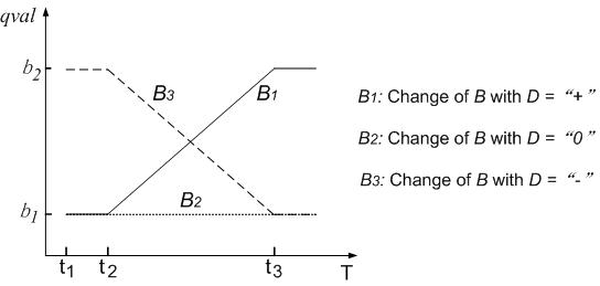
Figure 2. Change of B

Method

1.23

QSIM has so far mainly been used with physical systems, for which the initial value of variables and the course of change among those variables are deterministic. However, in contrast to most physical systems, group behavior systems have the following properties:

• Environmental factors are unsteady and tend to affect group behavior; and
• The motivation and behavior of an individual may change in unpredictable ways even in a working day.

1.24

Since the course of change among variables in employee group behavior is complex, QSIM cannot be used alone, but rather should be combined with other methods. Causal reasoning should also not be used alone, though historically it has often been in the physical and social sciences. As mentioned in Section 1.1, the behavior desired by managers from employee groups is expressed in the following ways:

• in Levels ("low", "moderate" or "high"); and
• in Change Directions ("decrease", "standard" or "increase").

1.25

The influence of both environmental and internal factors means that group behaviors are dynamic. For this reason we have combined the causal reasoning method with the state variable description approach of QSIM. Since "decrease", "standard" and "increase" are not exact values but rough directions (i.e. "-", "0" or "+"), we will be using a very basic causal graph.

1.26

Also, the simulated subject of this paper is a group, not an individual. When managers make decisions in regards to employees, they are generally thought of a single unit, as a "group", rather than as "individuals". The behavior of an individual tends to change abruptly while the behavior of a group tends to change gradually over time.

Description and Explanation of Group Behaviors

2.1

In order to explain the manner in which change occurs within a group, there are certain factors that must be taken into consideration. They are:

• The External Environment. The external environment includes political, economic, social and technical factors occurring outside of the enterprise.
• The Organizational Culture. The organizational culture refers to the culture within an enterprise. The components that make up the Organizational Culture of an enterprise include group morale, shared habits, the characteristics of the "leader(s)", and shared values.
• Management policies. i.e. strategies for employee motivation.
• Group Structure i.e. sub-groups (explained in detail below).

2.2

Employee group behavior is affected by these factors as illustrated in Figure 3. The external environment and management policies are viewed as "inputs". The resulting behavior is viewed as "output". The structure is formed by sub-groups within the whole. Organizational culture also affects group behavior, though it is not included in this illustration.

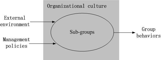
Figure 3. Schematic framework of an employee group system

Before deriving the QSIM description for the above factors and their complex relationships, we give an example.

An Example

2.3

In an enterprise there is what is called a Centre for Information Management (CIM). The role of the CIM is to maintain Management Information Systems (MIS) for the enterprise. The CIM is comprised of a group of individuals whose role is to develop a MIS for each department. It is difficult, however, to keep these systems up to date. When software updates are released into the IT market, previous versions quickly become obsolete. It is difficult for the CIM to keep up, since the new versions of software require those using it to update their skills to match it. Workers that are able to do this are the most in demand, and are also the highest paid. Therefore, once updated software has been released, those that have mastered it are likely to look for higher paying positions elsewhere.

2.4

Updated software is considered a change in the external environment. This changes the Organizational Culture of the enterprise, which in turn has a negative effect on the employee group. In order to prevent this change from affecting the group, managers will need to develop a pre-emptive strategy if they want to prevent corresponding changes to employee behavior.

Variables

2.5

There are three variables to take into consideration: the environment, decision and state variables. These represent environmental factors, management policies and employee group behavior, respectively.

2.6

Let X₁ be the environment variable, which will refer to the effect updated software has on the MIS. Let X₂ be the decision variable, which will refer to a manager's strategy for preventing unwanted resignations. Once new or updated software has been released, the manager of the CIM implements an incentives program: Those who master the new or updated software will win a prize. By rewarding skilled employees, the manager hopes to prevent the company losing their skills to other companies.

2.7

According to Brooks (2003), a group can be divided into several sub-groups: the leader, formal members, informal members and independent members. The leader dictates the change direction of the group as a whole. Most members of an employee group will follow the leader. Formal members make up the main body of the group; they obey all company rules and regulations, as well as those informally imposed by the leader. Informal members sometimes obey, but sometimes they do not. Independent members usually do not follow rules or regulations. They are individualistic and do not like to cooperate.

2.8

Let G₁, G₂, G₃ and G₄ be state variables, which refer to the properties of the leader, formal members, informal members, independent members and group, respectively. Let G refer to group cohesion. QS(F, t_i) and QS(F, t_i, t_i+1) refer to the qualitative value of variable F at time point t_i and in time interval (t_i, t_i+1), respectively. A time point means that F reaches a distinguished value at this time, i.e., the state variable reaches a distinguished value, or there is a change in the environment variable or decision variable.

2.9

In reference to environment and decision variables, we need to know their effect on the direction of the state variable (i.e., negative, no influence or positive). Therefore, X₁ and X₂ are expressed as:

QS(x, ti) = <qval>

(1)

where x ∈ {X₁, X₂}, t_i indicates that X₁ or X₂ changes only at a distinguished time point, t_i ∈ {t₀, t₁, ..., t_n } is a distinguished time point, qval ∈ {"-", "0", "+"}. For X₁, "-", "0" or "+" indicates negative, no influence or positive, respectively. For X₂, "-", "0" or "+" indicates low, moderate or high, respectively.

2.10

For example, QS(X₁, t_i) = <+> means that at the time point t_i, new software has been released into the market. QS(X₂, t_i) = <+> expresses that at the time point t_i, manager has implemented a new incentives program for employees that have updated their skills accordingly.

2.11

State variables G₁, G₂, G₃, G₄ or G are expressed as:

QS(f, ti) or QS(f, ti, ti+1) = <qval, qdir>

(2)

where f ∈ { G₁, G₂, G₃, G₄, G }, qval is the magnitude of f and qdir is its change direction. In qualitative simulation, the simulation clock is moved alternately to the time point and in the time interval, which are referred to as time stages. Therefore, the time stages are:
t₀, (t₀, t₁), t₁, (t₁, t₂), ......, t_i, (t_i, t_i+1), t_i+1, ......(t_n-1, t_n), t_n

2.12

To describe the behaviors and interaction between members of the employee group, qval and qdir are:

(3)

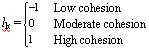
where l_j ={-1,0,1}. l_k is the landmark value of f, and is the same as the distinguished value of f. (l_k, l_k+1) indicates that the value of qval is between l_k and l_k+1.

qdir = {2-, -, 0, +, 2+}

(4)

where "-", "0" and "+" refer to change directions down, no change and up, respectively. "2" indicates that the change speed of f is very high. We use "2" to indicate the degree to which the cause variable affects f. When the cause variable has a great effect (negative or positive) on f, then the state variable in qdir is "2".

2.13

QS(G₁, t_i, t_i+1) = <(0, 1), 2+> for example, shows that at time point t_i, the environment variable or decision variable has a high positive effect on G₁. This means that the speed of change of G₁ is fast in the next time stage (t_i, t_i+1).

2.14

For state variables G₁, G₂, G₃ and G, l_k refers to:

(5)

2.15

For state variable G₄, l_k refers to:

(6)

2.16

For example, QS(G₂, t_i, t_i+1) = <(-1, 0), +> shows that the level of G₂ is (-1, 0) in time interval (t_i, t_i+1), its change direction is "+", and its change speed is moderate.

2.17

At distinguished time points, the qualitative value of the state variable changes (i.e. there is a change of magnitude or change direction). During the time intervals, the state variable changes only gradually.

2.18

For example, when new software is released (i.e. QS(X₁, t_i) = <+>), the time point t_i is a distinguished time point. Because of the change of X₁, the formal sub-group may show no more cohesion than before. Some members may have begun to consider looking outside the enterprise for a higher salaried position. In this case, the cohesion of formal sub-group G₁ will change to be "low". The change, however, will happen gradually, since the sub-group is not an individual. Individuals may make decisions quickly, but groups do not. When the environment changes, group members will take a period of time to discuss and consider one another's point of view before making a final decision. When a decision is finally made, either the magnitude or the change direction of the state variable will have a distinguished change. The point where the variable has a distinguished change will be the next distinguished time point t_i+1.

Description of behavior

2.19

According to Brooks (2003), changes of external or internal factors can have an effect on group behavior, causing it to change. However, in the absence of any further change of external or internal factors, group behavior will revert back to its original state. This is an important phenomenon in human resource management. Manager may achieve a degree of initial success in the promotion and maintenance of company loyalty by giving a pay increase. However, if nothing further is done to motivate company loyalty, after a period of time it will fall back to its original level.

2.20

This is expressed as follows: If X₁ or X₂ changes, the value of G₁, G₂, G₃, G₄ and G will change correspondingly. However, if X₁ or X₂ do not change again, G₁, G₂, G₃, G₄ and G will revert back to their original values.

2.21

Based on the above regularity, the causality between variables A and B is illustrated in Figure 4. It is derived from Figure 1. The effect on variable B is also illustrated in Figure 5 corresponding to Figure 2(a). Where L₁ ∈ {0, L^*}, L₂ ∈ {-1, 0, 1}, L^* is the new landmark value.

Figure 4. Causal graph used in this paper

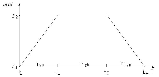
Figure 5. Transition of B with D="+"

2.22

The time point t₁ in Figure 1 is omitted in Figure 4. This means that if A (i.e. X₁ or X₂) changes, B (the state variable) will change immediately. There is no delay before B begins to change.

2.23

T_1gp refers to the duration between the time point when A begins to change and the time point when B stays at the landmark value L₂. T_1gp also refers to the duration of B's transition between landmark values L₂ to L₁. In this paper we assume these two time periods are equal. They are both T_1gp. T_2gh refers to the length of time B staying at landmark value L₂. D refers to the same as in Figure 1, i.e., the effect of A on B. D ∈ {-, 0, +}.

2.24

The parameters in T_1gp and T_2gh represent the properties of group dynamics and organizational culture.
"1" means that T_1gp indicates when B is in the process of change. In Figure 5, time periods (t₁, t₂) and (t₃, t₄) are dictated by T_1gp. The change direction of B is "increase" between L₁ and L₂ in (t₁, t₂), and "decrease" between L₂ and L₁.

"2" means that T_2gh dictates the length of time that B stays at a landmark value (does not change). In Figure 5, time period (t₂, t₃) is T_2gh. After B reaches L₂, it remains for the length of time referred to by T_2gh.

"g" represents the state variable. g ∈ {0, 1, 2, 3, 4}. "0", "1", "2", "3" and "4" indicate that B is G, G₁, G₂, G₃ and G₄, respectively. "p" represents the change speed of B. p ∈ {1, 2}. "1" means fast, "2" means slow. So in Figure 5, "1" indicates that the time period (t₁, t₂) or (t₃, t₄) is short, while "2" indicates that the period is long.

"h" represents the duration of T_2gh. h ∈ {0, 1, 2, ∞}. "0" indicates that T_2gh = 0 (B does not stay at L₂). Once it reaches L₂, it immediately returns to L₁. "1" indicates the T_2gh is a short period of time (B delays at L₂ for a short period of time). "2" indicates that T_2gh is a long period of time (B delays at L₂ for a long period of time). " ∞" indicates that T_2gh is an infinite period of time (B will never return to L₁).

"h" can be used to refer to the organizational culture of the enterprise. When D = "+", h ="1" indicates that the group is behaving normally, with slight variations. Once the state variable reaches the new landmark value, it will stay there for a short period of time, and then, will return to its original state. h ="2" indicates that the group is behaving normally with no variations. Once the state variable reaches the new landmark value, it will stay there for a long period of time. By using "h" this way we are able to illustrate the effect of organizational culture.

2.25

In this paper, D = "-" indicates group morale, which is another property of group that must be taken into consideration.
When D = "-", h = " ∞" indicates that B does not return to its original landmark value after it decreases to L₂. This is illustrated in Fig 6(a), showing low group morale.
When D= "-", h = "0" indicates that group morale is high, h = "1" indicates that it is moderate, and h = "2" indicates that it is low. These are each illustrated as Fig 6(b) (p ∈ {1, 2}, h ∈ {0, 1, 2}).

(a)

(b)

Figure 6. Transition of B with D = "-"

Distinguished Time Points and Landmark Values

2.26

Recall that a distinguished time point is a time point when a state variable has a distinguished change of magnitude or direction. A landmark value is the value of a state variable L ∈ {-1, 0, 1} at a distinguished time point. There are two cases during which new landmark values for state variable B may be generated:

1. At a time point, there is a change in environment or decision variables. This time point is now considered as a distinguished time point. At this time point, if the value of the state variable B is not L (L ∈ {-1, 0, 1}), then a new landmark value for B is generated (see Figure 7). In simulation runs, there are two scenarios that can cause state variable B to change direction: The release of updated software or a policy taken by a manager (i.e. incentives offered) at time point t^*. In either case a new landmark value L^* is generated at t^*.

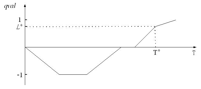
   Figure 7. The generation of the new landmark value L*

2. In simulation runs, suppose t_i is the distinguished time point of one state variable (cause variable A), and t_j is the distinguished time point of the other state variable (effect variable B). If t_i < t_j, then t_i is regarded as the new distinguished time point of B. At this time point the new landmark value L^* for B is generated. This case will be explained further in Section 4.

2.27

Figure 6(b) is an illustration of the state variable B. Between distinguished time points t₁ and t₄, the values of B are as follows: QS(B, t₁) = <L₁, 0>, QS(B, t₁, t₂) = <(L₂, L₁), ->, QS(B, t₂) = <L₂, 0>, QS(B, t₂, t₃) = <L₂, 0>, QS(B, t₃) = <L₂, 0>, QS(B, t₃, t₄) = <(L₁, L₂), +>, QS(B, t₄) = <L₁, 0>.

Group Behavior Causality

2.28

The example in Section 2 is the cause of an effect as illustrated in Figure 8. This is a series of causal graphs which illustrate the interactions between the three types of variable. The cause variables and effect variables are:

• X₁ and X₂ are cause variable A;
• o G is effect variable B; and
• o G₁, G₂, G₃ and G₄ are both cause and effect variables.

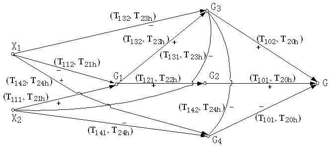
Figure 8. Group Behavior Causality

Figure 8 is not a generic model for all enterprises, but serves as an example for the illustration and validation of the proposed method.

2.29

In this example, the formal sub-group is not directly affected by the external environment or management policy since, according to Brooks (2003), the formal sub-group obeys the leaders. The Informal and independent sub-groups are in the minority. The independent sub-group is often regarded as being the source of negative group behavior and therefore the independent sub-group generally receives negative feedback that in actuality has been earned by the informal sub-group. In this paper, the aspects of group behavior that will be considered are "cohesion" and "independence" as defined in paragraph 2.8.

Qualitative Simulation Methods

3.1

In Figure 8, when environment X₁ or management policy X₂ changes, it leads to changes in the state variables at each time stage. What are these changes? How do state variables change? These answers can be found using the qualitative simulation method. In this section the rules and simulation engine of qualitative simulation are described.

The Rules

Rule 1: Parameter setup.
The external environment and the internal management policy of an enterprise both affect the group. Generally speaking, internal management policy has a much greater effect than what is external. Therefore, to determine T_1gp, let p = "1" to represent the causality between the decision variable and state variables, and let p = "2" to represent the causality between the environment variable and state variables.

Rule 2: Reasoning Sequence. In Figure 8, the reasoning sequence of variables runs from left to right. However, changes to state variables all happen at the same time and not from left to right.

Rule 3: Calculation of the change of direction of B. Let CDB be the change of direction of B. According to Figure 4, CDB depends on D and QS(A, t_i). If A is the environment or decision variable, the calculation of CDB is performed as illustrated by Table 1. For example, suppose A is X₁ and QS(X₁, t_i) = <+>, meaning that new or updated software has been released. Suppose B is G₃ (the cohesion of the informal sub-group). Therefore, if D = "-", then the CDB of G₃ is "-".
If A is a state variable, the calculation of CDB is done as illustrated by Tables 2 and 3. The state variable is expressed by a 2-tuple with qval and qdir, so CDB is calculated by qval or qdir. Since the value of qdir is expressed as either "-", "0" or "+", the way we calculate CDB using qdir in Table 2 is identical to the way it is done in Table 1.
However, the value of qval is expressed in three ways: "less than 0", "0" and "greater than 0" (See Table 3). These values are represented by "-", "0" and "+" respectively. Therefore, the way to calculate CDB using qval in Table 3 is also the same as Table 1.

Table 1: Calculation of CDB (if A is environment or decision variable)
QS(A, ti) D	-	0	+
-	+	0	-
0	0	0	0
+	-	0	+

Table 2: Calculation of CDB using qdir (if A is the state variable)
Qdir of QS(A, ti) D	-/2-	0	+/2+
-	+	0	-
0	0	0	0
+	-	0	+

Table 3: Calculation of CDB using qval (if A is state variable)
qval of QS(A, ti) D	-1	(-1,0)	0	(0,1)	1
-	+	+	0	-	-
0	0	0	0	0	0
+	-	-	0	+	+

Rule 4: Calculation of p.
When A is a state variable, during the change process of B, the values of p are calculated as follows:
IF qdir of A is "2+" or "2-", then p = "1"
IF qdir of A is "+" or "-", then p = "2"
IF qdir of A is "0", then B remains unaffected.
"2" indicates that the effect of A on B is great. This causes A to change quickly in the next time stage. So p = "1". If there is no "2" in qdir of A, then the effect is moderate, and p = "2".

Rule 5: State transition.
The state transitions of B are illustrated in Figure 9 according to the rules outlined above, and in which h is calculated according to the following:
IF CDB ="+" and the group is behaving normally with slight variations, then h = "1".
IF CDB ="+" and the group is behaving normally with no variations, then h = "2".
IF CDB ="-" and group morale is high, then h = "0".
IF CDB ="-" and group morale is normal, then h = "1".
IF CDB ="-" and group morale is low, then h = "2".
IF CDB ="-" and group morale is very low, then h = " ∞".
CDB = "+" shows that qval of B has increased. CDB = "-" shows that qval of B has decreased. The state transitions of B imply common group dynamics and organizational culture. Since group dynamics and organizational cultures are varied and complex, the possible ways in which B can change are varied. These possibilities are illustrated in subfigures of Figure 9.

Figure 9a. State transitions of B when CDB = "+", p = "2", h= "2"

Figure 9(a) illustrates a case where A has a moderate effect on B which causes the group to behave normally with no variations. This is expressed as p = "2" and h= "2". If p = "2", this indicates that B will take a long period of time to reach the landmark value L₂. Since h= "2" after B reaches L₂, it will stay at L₂ for a long period of time.

Figure 9b. State transitions of B when CDB = "+", p = "2", h= "1"

Figure 9(b) illustrates a case where A has a moderate effect on B which causes the group to behave normally with slight variations. This is expressed as p = "2" and h= "1". Since h= "1" after B reaches L₂, it will stay at L₂ for a short period of time.

Figure 9c. State transitions of B when CDB = "+", p = "1", h= "1"

Figure 9(c) illustrates a case where A has a great effect on B which causes the group to behave normally with slight variations. This is expressed as p = "1" and h= "1". Since p = "1", B will take a short period of time to reach the landmark value L₂.

Figure 9d. State transitions of B when CDB = "+", p = "1", h= "2"

Figure 9(d) illustrates a case where A has a great effect on B which causes the group to behave normally with no variations. This is expressed as p="1" and h= "2" which results in the same as above.

Figure 9e. State transitions of B when CDB = "-", p = "2", h = "0"

Figure 9(e) illustrates a case where A has a moderate effect on B and where group morale is high. This is expressed as p = "2" and h= "0". Since group morale is high (h= "0"), after B falls (decreases) to L₂, it will immediately increase back to its original value.

Figure 9f. State transitions of B when CDB = "-", p = "2", h= "1"

Figure 9(f) illustrates a case where A has a moderate effect on B and where group morale is normal. This is expressed as p = "2" and h= "1". Since group morale is normal after B falls to L₂, it will not increase immediately, but will do so over a short period of time.

Figure 9g. State transitions of B when CDB = "-", p = "2", h= "2"

Figure 9(g) illustrates a case where A has a moderate effect on B and where group morale is low. This is expressed as p = "2" and h= "2". Since group morale is low, after B falls, it will remain low for a long period of time.

Figure 9h. State transitions of B when CDB = "-", p = "2", h= " ∞"

Figure 9(h) illustrates a case where A has a moderate effect on B and where group morale is very low. This is expressed as p = "2" and h= " ∞". Since group morale is very low, after B falls, it will remain low indefinitely.

Figure 9i. State transitions of B when CDB = "-", p = "1", h= "0"

Figure 9(i) illustrates a case where A has a great effect on B and where group morale is high. This is expressed as p = "1" and h= "0".

Figure 9j. State transitions of B when CDB = "-", p = "1", h= "1"

Figure 9(j) illustrates a case where A has a great effect on B and where group morale is normal. This is expressed as p = "1" and h= "1".

Figure 9k. State transitions of B when CDB = "-", p = "1", h= "2"

Figure 9(k) illustrates a case where A has a great effect on B and where group morale is low. This is expressed as p = "1" and h= "2".

Figure 9l. State transitions of B when CDB = "-", p = "1", h= " ∞"

Figure 9(l) illustrates a case where A has a great effect on B and where group morale is very low. This is expressed as p = "1" and h= " ∞".

Rule 6: Time priority (the successor state filter).
When A affects B, B may have several successor states after transition. The function of this rule is to filter out anomaly successor states that do not exist in reality. This rule also determines the distinguished time point of B. The rule is as follows:
The distinguished time point of B is the time point at which a successor state reaches the landmark value first. The corresponding value on the Y-axis is the landmark value of B and all remaining successor states are filtered out. There are two variations on this rule:

• When the change direction of B qdir ≠ "0". If B has more than one cause variable, then the successor state that reaches the landmark value L₂ first is the successor state of B.
• When the change direction of B qdir = "0". The successor state for B is the successor state for which the value of T_2gh is the smallest.

Rule 7: State combination.
Following Rule 6, if the successor states of B have different qval and inconsistent qdir, then the following is applied in order to combine them.

is the number of successor states. Their mean values are:

Then the rules are:

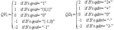
IF SQV<1 then B's qval = -1	IF SQD<1 then B's qdir = 2-
IF SQV=-1 then B's qval = (-1, 0)	IF SQD=-1 then B's qdir = -
IF SQV = 0 then B's qval = 0	IF SQD = 0 then B's qdir = 0
IF SQV = 1 then B's qval = (0, 1)	IF SQD = 1 then B's qdir = +
IF SQV > 1 then B's qval = 1	IF SQD > 1 then B's qdir = 2+

QV_i, QD_i are the variables used to combine the successor states of B after filtering. They are not applicable to actual employee group behavior.

Simulation engine

3.2

The initial values of state variables are: QS(G₁, t₀), QS(G₂, t₀), QS(G₃, t₀), QS(G₄, t₀) and QS(G, t₀).

• Step1: Determine successor states of the state variable according to Rule 2 and Rule 5 going from left to right in Figure 8.
• Step2: Choose the successor states for the effect variable B that have more than one cause variable by following Rule 6. The number of h in T_2gh may be more than one, so the number of successor states for the effect variable B will be more than one.
• Step 3: Filter out anomaly successor states according to Rule 6.
• Step 4: For the successor states whose qvals are different or qdirs are inconsistent, combine them according to Rule 7.
• Step 5: If G has been determined, go to Step 6. Otherwise, go to Step 2.
• Step 6: If the successor states return to their initial values, go to Step 8. Otherwise, go to Step 7.
• Step 7: Move the simulation runs to the next time stage (the next distinguished time point or an interval time), and then go to Step 1.
• Step 8: Stop simulation runs.

Validation of the proposed method

4.1

Now we will integrate all of the above components into a conceptual model of integrated qualitative simulation of group behavior. This model is illustrated in Figure 10.

4.2

The description method is the first component. When internal and external changes are input, the second component, The rules, becomes applicable. It is comprised of Transition of state, Filter of successor states and Combination of successor states. The Transition yields successor states. The Filter then prunes the anomalies. After that the remaining successor states are combined by the Combination.

4.3

The third component, the Qualitative simulation engine, drives the runs of other components.

Figure 10. Conceptual model of integrated qualitative simulation with inputs and outputs

4.4

In this Section, we discuss the validation of the conceptual model. There are two methods for testing validation: basic (quantitative) validation and qualitative validation (Dijkum et al 1999). The validation appropriate for our method is obviously qualitative. Because there is no standard means of testing the validation of a qualitative simulation method, in this paper we shall follow these steps:

• First, take an example of a group behavior system;
• Second, based on the example, set up an experimental design (i.e. changes of external environment and management policy);
• Third, run a simulation to obtain outputs (i.e. employee group behaviors); and
• Fourth, compare the inputs-outputs to predictions made in Brooks (2003). If the inputs-outputs are consistent with the predictions, the proposed integrated qualitative simulation is considered to be valid.

Experimental design

4.5

Figure 8 will be used for this example. The initial setup at time point t₀ is:

• Let QS(X₁, t₀) = <+>; (i.e. new or updated software which has a great effect on the MIS of the enterprise is released into the IT market) and
• Let QS(X₂, t₀) = <+>, (i.e. managers of the enterprise implement an incentive program to motivate specially skilled members of the CIM).

We assume that after the initial time point t₀, X₁ and X₂ will not change any further. The organizational culture of the enterprise is:

• The group behaves normally with no variations; and
• Group morale is normal.

Using the above experimental design, group behavior is simulated as follows.

Simulation runs

Initial value of state variables

QS(G₁, t₀) = <0, 0>, QS(G₂, t₀) = <0, 0>, QS(G₃, t₀)= <0, 0>, QS(G₄, t₀)= <0, 0>, QS(G, t₀) = <0, 0>. Let t₀ = 0. Then the time stages of simulation are timed from t₀ = 0.

t = (t_0, t₁)

(1)G₁
1)By X₁, QS(G₁, 0, t₁) = <(-1, 0), ->, where t₁ = T₁₁₂
2)By X₂, QS(G₁, 0, t₁)= <(0, 1), +>, where t₁ = T₁₁₁
According to Rule 6, choose X₂ as the cause variable where t₁ = T₁₁₁.

(2)G₃
1)By X₁, QS(G₃, 0, t₁)= <(-1, 0), -> where t₁ = T₁₃₂
2)By G₁, QS(G₃, 0, t₁)= <(0, 1), +> where t₁ = T₁₃₂
3)By X₂, QS(G₃, 0, t₁) = <(-1, 0), -> where t₁ = T₁₃₁
Choose X₂ as the cause variable where t₁ = T₁₃₁.

(3)G₂
By G₁, QS(G₂, 0, t₁)= <(0, 1), +> where t₁ = T₁₂₁.

(4)G₄
1)By X₁, QS(G₄, 0, t₁)= <(0,1),+> where t₁ = T₁₄₂
2)By X₂, QS(G₄, 0, t₁)= <(-1,0),-> where t₁ = T₁₄₁
3)By G₃, QS(G₄, 0, t₁)= <(0,1),+> where t₁ = T₁₄₂
Choose X₂ as the cause variable where t₁ = T₁₄₁.

(5)G
1)By G₂, QS(G, 0, t₁)= <(0,1),+> where t₁ = T₁₀₁
2)By G₃, QS(G, 0, t₁)= <(-1,0),-> where t₁ = T₁₀₂
3)By G₄,QS(G, 0, t₁)= <(0,1),+> where t₁ = T₁₀₁
Therefore combine QS(G, 0, t₁)= <(0, 1), +> where t₁ = T₁₀₁.

We will use one example from the above to help clarify the meaning of the simulation as a whole. We will use number 1: "By X₁, QS(G₁, 0, t₁) = <(-1, 0), ->, where, t₁ = T₁₁₂".

"By X₁" refers to the effect had by X₁ on state variable G₁. "QS(G₁, 0, t₁) = <(-1, 0), ->" shows that the value of G₁ has been affected and changed to <(-1, 0), -> ) in the time interval (0, t₁) from QS(G₁, t₀) = <0, 0>. "T₁₁₂" is a time period as is previously explained. However, it is used here to record the time of t₁. It indicates that the time period from 0 to t₁ is T₁₁₂. Therefore t₁ is a fuzzy time point. We do not know the exact duration, only that the period of time between 0 and T₁₁₂ is long. We know this because p = "2".

Now t₁ = T₁₀₁. This indicates that the time period between 0 and t₁ is T₁₀₁.

t = t₁

(1)QS(G₁,t₁)= <1, 0> where t₁ = T₁₁₁
(2)QS(G₃,t₁)= <-1, 0> where t₁ = T₁₃₁
(3)QS(G₂,t₁)= <1, 0> where t₁ = T₁₂₁
(4)QS(G₄,t₁)= <-1, 0> where t₁ = T₁₄₁
(5)QS(Y, t₁)= <1, 0> where t₁ = T₁₀₁

t = (t₁, t₂)

(1)G₁
QS(G₁, t₁, t₂)= <1, 0> where t₂ = T₁₁₁+T₂₁₂
(2)G₃
By G₁, QS(G₃, t₁, t₂)= <(-1,0),+> where t₂ = T₁₃₁+T₁₃₁
(3)G₂
By G₁, QS(G₂, t₁, t₂)= <1, 0> where t₂ = T₁₂₁+T₁₂₁
(4)G₄
By G₃, QS(G₄, t₁, t₂)= <(-1,0),+> where t₂ = T₁₄₁+T₁₄₁
(5)G
1)By G₃, QS(G, t₁, t₂)= <1,0> where t₂ = T₁₀₁+T₁₀₂
2)By G₂, QS(G, t₁, t₂)= <1,0> where t₂ = T₁₀₁+T₁₀₁
3)By G₄, QS(G, t₁, t₂)= <(0,1),-> where t₂ = T₁₀₁+T₁₀₁
Therefore combine QS(G, t₁, t₂)= <1,0> where t₂ = T₁₀₁+T₁₀₁
This shows that the time period between 0 and t₂ is T₁₀₁+T₁₀₁. Later time points are also shown in this way.

t = t₂

(1)QS(G₁, t₂)= <1, 0> where t₂ = T₁₁₁+T₂₁₁
(2)QS(G₃, t₂)= <0, 0> where t₂ = T₁₃₁+T₁₃₁
(3)QS(G₂, t₂)= <1, 0> where t₂ = T₁₂₁+T₁₂₁
(4)QS(G₄, t₂)= <0,0> where t₂ = T₁₄₁+T₁₄₁
(5)QS(G, t₂)= <1, 0> where t₂ = T₁₀₁+T₁₀₁

t = (t₂, t₃)

(1)G₁
QS(G₁, t₂, t₃)= <1,0> where t₃ = T₁₁₁+T₂₁₂
(2)G₃
By G₁, QS(G₃, t₂, t₃)= <(0,1), +> where t₃ = T₁₃₁+T₁₃₁+T₁₃₂
(3)G₂
By G₁, QS(G₂, t₂, t₃)= <1, 0> where t₃ = T₁₂₁+T₁₂₁+T₁₂₁
(4)G₄
By G₃, QS(G₄, t₂, t₃)= <(-1, 0),-> where t₃ = T₁₄₁+T₁₄₁+T₁₄₂
(5)G
1)By G₃, QS(G, t₂, t₃))= <1, 0> where t₃ = T₁₀₁+T₁₀₁+T₁₀₂
2)By G₂, as above.
3)By G₄, as above.
Therefore combine QS(G, t₂, t₃)= <1, 0> where t₃ = T₁₀₁+T₁₀₁+T₁₀₁

According to Rule 6, because T₁₃₂>T₁₃₁, time point t₃ = T₁₃₁+T₁₃₁+T₁₃₁, and G₃ generates a new landmark value L^*₃₁. QS(G₃, t₂, t₃) = <(0, L^*₃₁), +> where t₃ = T₁₃₁+T₁₃₁+T₁₃₁.

Because T₁₄₂>T₁₄₁, time point t₃ = T₁₄₁+T₁₄₁+T₁₄₁, and G₄ generates a new landmark value L^*₄₁, QS(G₄, t₂, t₃)= <(-1, L^*₄₁), -> where t₃ = T₁₄₁+T₁₄₁+T₁₄₁.

t = t₃

(1)QS(G₁, t₃)= <1, 0> where t₃ = T₁₁₁+T₂₁₂
(2)QS(G₃, t₃)= < L^*₃₁, 0> where t₃ = T₁₃₁+T₁₃₁+T₁₃₁
(3)QS(G₂, t₃)= <1, 0> where t₃ = T₁₂₁+T₁₂₁+T₁₂₁
(4)QS(G₄, t₃)= <L^*₄₁, 0> where t₃ = T₁₄₁+T₁₄₁+T₁₄₁
(5)QS(G, t₃)= <1, 0> where t₃ = T₁₀₁+T₁₀₁+T₁₀₁

t = (t_3, t₄)

(1)G₁ QS(G₁, t₃, t₄)= <(0, 1), -> where t₄ = T₁₁₁+T₂₁₂+T₁₁₁
(2)G₃
By G₁, QS(G₃, t₃, t₄)= <(0, L^*₃₁), -> where t₄ = T₁₃₁+T₁₃₁+T₁₃₁+ T₁₃₂
(3)G₂
By G₁, QS(G₂, t₃, t₄)= <(0, 1), -> where t₄ = T₁₂₁+T₁₂₁+T₁₂₁+ T₁₂₁
(4)G₄
By G₃, QS(G₄, t₃, t₄)= <(L^*₄₁, L^*₄₂), +> where t₄ = T₁₄₁+T₁₄₁+T₁₄₁+ T₁₄₂
(5)G
1)By G₃, QS(G, t₃, t₄)= <(0, 1), -> where t₄ = T₁₀₁+T₁₀₁+T₁₀₁+ T₁₀₂
2)By G₂, QS(G, t₃, t₄)= <(0, 1), -> where t₄ = T₁₀₁+T₁₀₁+T₁₀₁+ T₁₀₁
3)By G₄, QS(G, t₃, t₄)= <1, 0> where t₄ = T₁₀₁+T₁₀₁+T₁₀₁+ T₁₀₁
Therefore combine QS(G, t₃, t₄)= <(0, 1), -> where t₄ = T₁₀₁+T₁₀₁+T₁₀₁+ T₁₀₁.

Because T₁₃₂>T₁₃₁, time point t₄ = T₁₃₁+T₁₃₁+T₁₃₁+T₁₃₁, and G₃ generates a new landmark value L^*₃₂, QS(G₃, t₃, t₄)= <(0, L^*₃₂), -> where t₄ = T₁₃₁+T₁₃₁+T₁₃₁.

Because T₁₄₂>T₁₄₁, time point t₄ = T₁₄₁+T₁₄₁+T₁₄₁+T₁₄₁, and G₄ generates a new landmark value L^*₄₂.

t = t₄

(1)QS(G₁, t₄)= <0, 0> where t₄ = T₁₁₁+T₂₁₂+T₁₁₁
(2)QS(G₃, t₄)= <L^*₃₂, -> where t₄ = T₁₃₁+T₁₃₁+T₁₃₁+T₁₃₁
(3)QS(G₂, t₄)= <0, 0> where t₄ = T₁₂₁+T₁₂₁+T₁₂₁+T₁₂₁
(4)QS(G₄, t₄)= < L^*₄₂, +> where t₄ = T₁₄₁+T₁₄₁+T₁₄₁+T₁₄₁
(5)QS(Y, t₄)= <0, 0> where t₄ = T₁₀₁+T₁₀₁+T₁₀₁+T₁₀₁

In this simulation run, T_1g1, T_2g1 represent a short period of time (because p = "1"). T_1g2, T_2g2 represent a long period of time (because p = "2"). The results are listed in table 4.

Table 4: Simulation results
	QS(G1, t)	QS(G2, t)	QS(G3, t)	QS(G4, t)	QS(G, t)
T = t0	<0, 0>	<0, 0>	<0, 0>	<0, 0>	<0, 0>
T =(t0, t1)	<(0, 1), +>	<(0, 1), +>	<(-1, 0), ->	<(-1, 0), ->	<(0, 1), +>
T = t1	<1, 0>	<1, 0>	<-1, 0>	<-1, 0>	<1, 0>
T =(t1, t2)	<1, 0>	<1, 0>	<(-1, 0), +>	<(-1, 0), +>	<1, 0>
T = t2	<1, 0>	<1, 0>	<0, 0>	<0, 0>	<1, 0>
T =(t2, t3)	<1, 0>	<1, 0>	<(0, L*31), +>	<(-1, L*41), ->	<1, 0>
T = t3	<1, 0>	<1, 0>	< L*31, 0>	<L*41, 0>	<1, 0>
T =(t3, t4)	<(0, 1), ->	<(0, 1), ->	<(0, L*32), ->	<(L*41, L*42), +>	<(0, 1), ->
T = t4	<0, 0>	<0, 0>	<L*32, ->	< L*42, +>	<0, 0>

Note: State variable G₃ and G₄ generate new landmark values, which are noted as asterisks.

Analysis of Simulation Results

4.6

In the above example, when X₁ and X₂ change at the initial time t = t₀, group behavior begins to change. Between the initial time point t = t₀ and t = t₄, there are eight transitions. When the simulation arrives at t = t₄, group behavior has nearly returned to its initial values (as shown in Table 4). For further analysis, Table 4 is represented graphically in Figure 11.

Figure 11. Change process of state variables

4.7

From Figure 11, we can analyze the simulation results in detail:

• Changes in the behavior of the leader and formal sub-group are the same as that of the group as a whole. This indicates that the leader and formal sub-group are the majority and that they determine the principal change in direction of the group.
• The informal and independent sub-groups do not always follow the rules and regulations followed by the group as a whole. Therefore the behaviors of these two groups easily generate new landmark values which deviate from the specified landmark value set {-1, 0, 1}.
• Sometimes the behaviors of the informal sub-group are on the upside of the x-axis which has a positive effect on the group overall. Sometimes their behaviors are on the downside of the x-axis which has a negative effect. This means that the informal sub-group is an unsteady sub-group for the group as a whole.

4.8

The above simulation results are consistent with the proposals in Brooks (2003): when managers are able to motivate their employees successfully, the overall efficiency of those employees will improve. However, if managers do not repeatedly motivate their employees, the overall efficiency will fall back to its original level.

Application of the proposed method

5.1

In this section we apply the proposed method to the development of motivational strategies by the managers of an employee group. We use Figure 8 as the example. There are many ways by which managers can motivate their employees to maintain favorable behavior overall. Two possible alternatives, according to Figure 11, are:

1. Implement a new motivational strategy at time point t₃.
2. Implement a new motivational strategy at time point t₄.

5.2

Possible motivational strategies include increasing salaries, improving work conditions, providing training opportunities, etc. We will not go into further detail about possible motivational strategies except to express them as follows: QS(X₂, t₃) = <+> or QS(X₂, t₄) = <+>.

5.3

Which alternative will produce the most favorable results? We will apply the proposed method in order to make our decision.

5.4

The results of the simulation run using Alternative 1 and Alternative 2 are as shown in Table 5 and 6, respectively. Graphic representations of these results are shown in Figures 12 and 13.

Table 5: Simulation results of Alternative 1
	QS(G1, t)	QS(G2, t)	QS(G3, t)	QS(G4, t)	QS(G, t)
T =(t3, t4)	< L*, 0>	< L*, 0>	<(L*31, 1), +>	<(L*41, 0), +>	< 1, 0>
T = t4	< L*, 0>	< L*, 0>	<1, 0>	< 0, 0>	< 1, 0>
T =(t4, t5)	<( L*,1), +>	<( L*,1), +>	<1, 0>	<(L*41, 0), ->	< 1, 0>
T = t5	<1, 0>	<1, 0>	<1, ->	<L*41, 0>	<1, 0>
T =(t5, t6)	<(0,1), ->	<(0,1), ->	<(L*32, 1), ->	<(L*41, L*42), +>	<(0,1), ->
T = t6	<0, 0>	<0, 0>	<L*32, 0>	<L*42, 0>	<0, 0>

Note: L^*, L^*₃₁, L^*₃₂, L^*₄₁ and L^*₄₂ are new landmarks value for state variables.

Table 6: Simulation results of Alternative 2
	QS(G1, t)	QS(G2, t)	QS(G3, t)	QS(G4, t)	QS(G, t)
T =(t4, t5)	<(0,1), +>	<(0,1), +>	<L*32, 0>	<L*42, +>	<(0,1), +>
T = t5	<1, 0>	<1, 0>	<L*32, 0>	< 0, 0>	<1, 0>
T =(t5, t6)	<1, 0>	<1, 0>	<( L*32, L*31), 0>	<(L*41, 0), ->	<1, 0>
T = t6	<1, 0>	<1, 0>	<L*31, 0>	<L*41, 0>	<1, 0>
T =(t6, t7)	<(0,1), ->	<(0,1), ->	<( L*32, L*31), ->	<(L*41, L*42), +>	<(0,1), ->
T = t7	<0, 0>	<0, 0>	<L*32, ->	<L*42, 0>	<0, 0>

Note: L^*₃₁, L^*₃₂, L^*₄₁ and L^*₄₂ are new landmarks value for state variables.

Figure 12. Illustration of Alternative 1

Figure 13. Illustration of Alternative 2

5.5

By analyzing and comparing the results as illustrated in Figure 12 and Figure 13, we can conclude the following:

• The behavior of G₁ and G₂ resulting from Alternative 1 is a little better than that resulting from Alternative 2, since L^*>0. The difference, however, is only slight.
• The behavior of G₃ resulting from Alternative 1 is a little better than that in Alternative 2, since L^*₃₂ <1, but the difference here is also very small.
• The resulting behavior of G₄ in Alternative 1 and in Alternative 2 is almost the same.
• The resulting behavior of G in Alternative 1 is better than that in Alternative 2, since 1>0.

Alternative 1 is better than Alternative 2 overall. Managers should therefore implement Alternative 1.

Conclusions and further work

6.1

In this paper our research is applied and presented in two parts:

1. A description method for interactions between three types of variables; and
2. A qualitative simulation method.

6.2

The description method is the key to qualitative simulation. The ways in which employee groups interact are related to their awareness of the external environment, management regulations, and group dynamics (Brooks 2003). They are ambiguous, subjective, incomplete and often invisible. Therefore, a perfect description method - one which describes these interactions precisely and completely - does not exist. It is possible, however, for us to formulate a description method that can be adjusted case by case, and that can provide a correct if not exact analysis of an employee group. In human resource management, managers generally base decisions on qualitative information rather than on precise numerical information. Qualitative information with different fuzzy levels and change directions is usually adequate. Therefore, we have integrated the description method of QSIM with a basic causal graph. This integration has the following advantages: o

• QSIM was developed and has already been used in the analysis of physical systems. By integrating QSIM with a basic causal graph, QSIM may be used in human resource management.
• A basic causal graph is too simplistic to break down complex challenges on its own. It is, however, a valuable enhancement to QSIM.

6.3

Based on the description method, we have designed a qualitative simulation method. It includes:

• The rules of qualitative simulation; and
• A qualitative simulation engine.

6.4

Through validation and application we have shown that the method proposed in this paper can serve as a valuable tool for virtual experimentation. It can be used to predict changes in employee group behavior and to aid in decision making on employee group management.

6.5

Further research should seek to improve the following:

• Description of interactions.
  In this paper, interactions between the three types of variables are described by integrating the QSIM method with a basic causal graph. For the complex interactions found in real-world enterprises, the basic causal graph as illustrated in Figure 2 seems to be somewhat naive. QSIM should be integrated with a more comprehensive causal reasoning method (Pearl 2000) in order to provide a more detailed analysis.
• Description of time delay.
  The time interval during which the state variable is undergoing change, and remains at a landmark value, is expressed in this paper as p ∈ {1, 2} and h ∈ {0, 1, 2, ∞} respectively. These descriptions are very fuzzy. In the field of qualitative simulation, the adequate description of a time delay is a common problem. Solving this problem would much improve our proposed method.

Acknowledgements

This work has taken place in the Qualitative Simulation Team Work for Complex Management Systems at the Modern Management Institute, Management College, Huazhong University of Science and Technology. It is supported by the China National Nature Science Fund (No.70271029) and the Hubei Province Nature Science Fund of China (2004ABA069). The authors would like to thank the anonymous referees for their comments and suggestions on early versions of this paper.

References

BERNDSEN R (1995), Causal Ordering in Economic Models. Decision Support Systems, 1995,15:157-165.

BERNDSEN R, Daniels H (1994), Causal Reasoning and Explanation in Dynamic Economic Systems. Journal of Economic Dynamics and Control, 1994,18:251-271.

BERENDS R, Romme G (1999), Simulation as a Research Tool in Management Studies. European Management Journal, 1999, 17(6):576-583.

BROOKS I (2003), Organisational behavior: individuals, groups and organization. Harlow: FT Prentice Hall, 2003.

CEM Say A C, Akyn H L (2003), Sound and complete qualitative simulation is impossible. Artificial Intelligence, 2003, 149: 251-266.

CLANCY J D, Kuipers J B (1998), Qualitative Simulation as a Temporally-extended Constraint Satisfaction Problem. Proceedings of the Fifteenth National Conference on Artificial Intelligence(AAAI-98), Cambridge, Ma: AAAI/MIT Press, 1998.

DIJKUM C, DeTombe D and Kuijk E (1999), Validation of Simulation Models. Amsterdam: SISWO (SISWO Publication 403), 1999.

GLYMOUR C (2003), Learning, prediction and causal Bayes nets. TRENDS in Cognitive Sciences, 2003, 7(1):43-48.

GUERRIN F, Dumas J (2001), Knowledge representation and qualitative simulation of salmon redd functioning Part I: qualitative modeling and simulation. BioSystems, 2001, 59:75-84.

IWASAKI Y (1988), Causal Ordering in a Mixed Structure. Proceedings of the Seventh National Conference on Artificial Intelligence(AAAI-88), St Paul, Minnesota,1988:313-318.

IWASAKIY, Y and Simon H A (1986), Causality in design behavior. Artificial Intelligence, 1986, 29(1):3-32.

KUIPERS J B (1986), Qualitative Simulation. Artificial Intelligence. 1986,29:289-338.

KUIPERS J B (1993), Qualitative Simulation: Then and Now. Artificial Intelligence, 1993, 59:133-1140.

KUIPERS J B (1993), Reasoning with qualitative models. Artificial Intelligence, 1993, 59:125-132.

KUIPERS J B (1994), Qualitative Reasoning: Modeling and Simulation with Incomplete Knowledge, Artificial Intelligence, MIT Press, Cambridge, MA, 1994.

LIN K P, Farley A M (1995), Causal reasoning in Economic Models. Decision Support Systems, 1995,15:167-177.

PEARL J (2000), Causality: Models, Reasoning, and Inference. Cambridge University Press, Cambridge, 2000.

PLATZNER M, Rinner B, Weiss R (1997), Parallel Qualitative Simulation. Simulation Practice and Theory, 1997, 5 (7-8):623-638.

PLATZNER M, Rinner B (2000), Toward Embedded Qualitative Simulation: A Specialized Computer Architecture for QSIM. IEEE Intelligent System, 2000, March/April: 62-68.

SALVANESCHI P, Cadei M, Lazzari M (1997), A Causal Modelling Framework for the Simulation and Explanation of the behavior of Structure. Artificial Intelligence in Engineering, 1997, 11:205-216.

SHEN Q and Leitch R R (1993), Fuzzy Qualitative Simulation. IEEE Trans. Syst. Man & Cybernet, 1993, 23.

WELD D (1990), Exaggeration. Artificial Intelligence, 1990, 43: 311-368.

Return to Contents of this issue

© Copyright Journal of Artificial Societies and Social Simulation, [2005]