Phillip Stroud, Sara Del Valle, Stephen Sydoriak, Jane Riese and Susan Mniszewski (2007)

Spatial Dynamics of Pandemic Influenza in a Massive Artificial Society

Journal of Artificial Societies and Social Simulation vol. 10, no. 4 9
<https://www.jasss.org/10/4/9.html>

For information about citing this article, click here

Received: 13-Apr-2007    Accepted: 14-Jun-2007    Published: 31-Oct-2007

Abstract

EpiSimS is a massive simulation of the movements, activities, and social interactions of individuals in realistic synthetic populations, and of the dynamics of contagious disease spread on the resulting social contact network. This paper describes the assumptions and methodology in the EpiSimS model. It also describes and presents a simulation of the spatial dynamics of pandemic influenza in an artificial society constructed to match the demographics of southern California. As an example of the utility of the massive simulation approach, we demonstrate a strong correlation between local demographic characteristics and pandemic severity, which gives rise to previously unanticipated spatial pandemic hotspots. In particular, the average household size in a census tract is strongly correlated with the clinical attack rate computed by the simulation. Public heath agencies with responsibility for communities having relatively high population per household should expect to be more severely hit by a pandemic.

Keywords:

Agent Based Modeling, Computer Simulation, Epidemic Simulation, Public Health Policy

Introduction

Overview of the EpiSimS Approach

1.1

EpiSimS simulates the daily trips and activities of 18.8 million synthetic individuals. These individuals move about on a synthetic landscape consisting of 2.3 million locations. Each location represents a physical place, such as an office building, a school building, or a city half-block. Each location is subdivided into sublocations that represent individual households, classroom mixing groups, workgroups, etc. in which person-to-person transmission opportunities occur. As individuals arrive at and depart from sublocations, the simulation develops the dynamic contact network by recording the amount of time each individual overlaps with each other person. The simulation computes the spatially-distributed spread of contagious disease by probabilistic disease transmission based on the contact times between infectious and susceptible persons.

1.2

The artificial society is partitioned into 6.3 million synthetic households. The distributions of household characteristics (e.g. the number of households with two adults and two students, where the age of the householder is between 35 and 40, where the household income is between $120,000 and $130,000) match actual demographic statistics in each of 12,226 US Census block-groups covering six southern California counties. Each individual has a schedule of daily activities; each activity has a specified start and stop time and a specified location. The activities undertaken by members of a synthetic household are drawn from the 60,000 activity surveys from actual households in the National Household Transportation Survey (USDOT 2003).

1.3

Each of the 938,000 southern California businesses, schools, restaurants, shops, hospitals, etc. listed in the Dun & Bradstreet business directory database is represented as a synthetic location. EpiSimS assigns a location to each non-household activity of each individual using a two-stage gravity model. The model ensures that the number of workers assigned to each work location matches the Dun & Bradstreet data, and that the distribution of commute distances from home to work matches the distribution extracted from the NHTS data.

1.4

An infected person progresses stochastically through a set of 14 disease states. For consistency with the National Pandemic Influenza Planning Scenario (USDHHS 2005; HSC 2006), this analysis is based on disease characteristics approximating those of the 1918-1920 influenza pandemic. The assumed pandemic influenza would sicken 90 million Americans and cause 1.8 million fatalities, in the absence of interventions.

1.5

EpiSimS can simulate various pharmaceutical and non-pharmaceutical interventions, including panic-based stay-home behavior, therapeutic and prophylactic use of antivirals, contact tracing, vaccination, wearing of masks, social distancing behaviors (increased inter-personal separation, hand washing, cough etiquette, etc.), household quarantine, and closures of schools. However, the results presented here are for a scenario where no interventions occur.

1.6

EpiSimS runs as a distributed simulation on hundreds of processors. Each processor takes care of computations for a subset of the locations. Each processor has an event handler that maintains a time-ordered event queue. Arrival events spawn departure events, which in turn spawn arrival events. There are also disease-related events. Movement of individuals between locations assigned to different processors is done by passing asynchronous messages.

1.7

EpiSimS has a unique capability to model realistic spatially-varying demographic characteristics. The massive agent-based approach simulates phenomena occurring over a range of scales. Disease progression is modeled at the individual level. Transmission is modeled at the level of a mixing group, where the contact time between two individuals is determined by how much time they overlap in the sublocation. Daily movement and activity of individuals is modeled at the location level, where the scale describing a location (city half-block or building) is appropriate to the mobility and activity data (NHTS surveys). The artificial society is constructed to exhibit spatial variation of demographic characteristics, tied to demographic data at the granularity of the US Census block-group (typically containing 1500 residents). Large-scale effects are captured by simulation of a sub-national semi-closed region representing more than 6% of the US population. As a result, the simulation generates spatial variation in the simulated pandemic severity that had not been anticipated with previous models. The simulation can quantify the correlation between local demographic characteristics and local pandemic severity, which can have ramifications for pandemic planning.

Historical Note

1.8

EpiSimS began at Los Alamos National Laboratory in 2000, and is an ongoing research effort. The use of massive simulation of individual agents to generate social contact networks has been described (Eubank 2004,Barrett 2005). EpiSimS originated as an extension of Transims (Smith 1995), which is a massive urban-area traffic simulation developed at Los Alamos National Laboratory. EpiSimS extends Transims by modeling disease progression in infected individuals, by implementing a sublocation mixing model, and by modeling disease transmission between individuals that occupy the same sublocation at the same time. In January 2005, EpiSimS split into two independent efforts, one at Virginia Biotechnology Institute, and the other remaining at Los Alamos. Since then, the Los Alamos EpiSimS engine has implemented a pandemic influenza disease model and a suite of interventions and reactive behaviors. Los Alamos has also constructed a sequence of synthetic populations, culminating with the southern California population described here. This report describes the Los Alamos EpiSimS effort, and makes no assertions regarding EpiSimS work at VBI.

Comparison to Other Simulations

1.9

Two other disease spread modeling efforts use the massive simulation approach. Epicast is a simulation in which the synthetic population consists of 140,500 identical structured communities of 2000 individuals each (Germann 2006). Each community has 855 households, four neighborhoods, one high school, one middle school, four elementary schools, and some play groups for preschoolers. Individuals mix at home each night, and in a mixing group (work or school) during the day. Each of 43,323 census tracts in the US are assigned one or more of these communities, depending on the number of people that live in the census tract. US Census tract-to-tract worker flow data is used to move workers from their tract of residence at night to their tract of work during the day. Because each community has an identical distribution of household size and identical values of other demographic measures, spatial variation in pandemic severity due to spatially varying demographics is not seen.

1.10

Another approach to simulating disease spread in massive artificial societies constructs the synthetic population to match Landscan data (Ferguson 2006). The Landscan data uses a worldwide spatial grid of 30 arc-second cells (approximately 1 km square), and uses satellite imagery and other data to estimate the number of people that occupy in each grid cell. They constructed synthetic households, schools, and workplaces, but made the assumption that "household size and age distributions did not vary geographically." Population movement is computed to match commuting distance distributions and long-range travel patterns. They observed spatial variation in the timing of the pandemic peak, but did not report spatial variation in the clinical attack rate.

1.11

Disease spread has been modeled in artificial societies that consist of individuals residing in cells on a two dimensional lattice, each having connections to his or her Von Neumann or Metropolis neighbors (Eidelson 2004), but such an approach is not intended to capture a realistic contact network. Another agent-based approach has individuals residing on a 2-D lattice and computes interactions according to spatial proximity of residence, but also allows individuals to interact non-locally based on mutual activities (Huang 2004; Dunham 2006). These approaches create social networks through rules and simple models, and are not based in actual demographics. Many analysts have examined disease spread on pre-structured social contact networks (Halloran 2002; Kretzschmar 2004; Glass 2006) but have ignored spatial dimensions, reporting temporal results only.

1.12

Viboud (2006) examined the timing of historical seasonal influenza epidemics by U.S. state. She notes influenza epidemics start in California more often than any other state, and attributes this to California's large population. We note that California's average household size is significantly higher than the US average, and suggest this as an alternative explanation.

Current Limitations of the EpiSimS Simulation

1.13

EpiSimS employs a set of simplifications, approximations, and assumptions that are gradually being improved. The synthetic population of southern California represents only individuals reported as household residents in the 2000 US Census. It does not represent the 2.11% of the population reported as living in group quarters (e.g. jails, dorms, nursing-care facilities). It is not clear to what extent the synthetic population captures the activity patterns of the undocumented population, which made up an estimated 6.5% of the California population in 2000 (USINS 2003). The artificial society does not include visiting tourists, and does not explicitly treat guests in hotels or travelers in airports.

1.14

In EpiSimS, weekdays and weekend days are averaged to get a representative day (during which 5/7 of the population engage in their weekday activities, and 2/7 engage in their weekend activities.) Also, summer schedules are averaged in with school year schedules. The result of this approximation is that on a given simulated day, roughly half of students are in school, and less than 5/7 of workers are at work.

1.15

Based on an assumption that influenza transmission from patients to medical personnel could be prevented by protective measures, EpiSimS does not yet model disease transmission between patients and medical personnel. Except for carpools, EpiSimS does not capture disease transmission during travel. EpiSimS does not yet properly model daycare. Preschoolers with daycare activity are effectively modeled as though they were workers.

1.16

If the activity schedules of an infectious person and a susceptible person result in them both being at the same location for some amount of time, and the EpiSimS sublocation model places them both in the same sublocation, then these two individuals are assumed to be in full contact until one of them leaves the location. Thus, two members of a household might be in contact for 12 hours, even though they would spend 8 hours sleeping in separate bedrooms. Similarly, two co-workers might be counted as spending 5 hours together even though they might spend a small fraction of that time face-to-face. Although EpiSimS has provisions for a user to adjust the relative strength of contact of each activity type for each demographic group, data do not exist to justify such adjustment factors. It is therefore quite possible for EpiSimS to overestimate (for household members that sleep in different bedrooms) or underestimate (for spouses) the household transmission. Nevertheless, EpiSimS obtains a fraction of infections acquired at home that is in rough agreement with other published results (Ferguson 2006, Germann 2006,Longini 2004), which suggests that the correlation we observe between average household size and local disease severity is more than an artifact of our assumptions.

Methodology

Construction of the Artificial Society

2.1

The methodology used to construct the synthetic population from census data, to assign activities to individuals based on household activity surveys, and to assign locations to activities, has been described and characterized in detail (Beckman 1995). Additional details about the artificial society used in this analysis are presented here.

The Synthetic Individuals

2.2

A synthetic population was constructed to match the actual population (USCB 2000) of six southern California counties (Los Angeles, Orange, San Diego, Riverside, San Bernardino and Ventura). It consists of 18,828,569 individuals. There are a total of 6,345,751 households, of which 1,455,712 are individuals living alone, 1,532,985 are married couples with children living at home, and the rest are various combinations of adults, seniors, preschoolers and students.

2.3

The US Census subdivides these six counties into 3978 census tracts, which are further subdivided into 12,226 census block groups. In each block-group, the synthetic population matches the actual population in several statistical measures: the number of residents, the number of households, the householder's age distribution, the household size and membership distribution, the household income distribution, number of workers, and the number of vehicles.

2.4

8,036,841 synthetic individuals are designated as workers, representing 42.7% of the population. The percentage of population in the workforce varies considerably from place to place. On a simulated day, 5.9 million workers will be working, and the other 2.1 million workers will not be working. There are 4.30 million students (age 5 to 18 inclusive) in the southern California synthetic population, making up 22.8% of the population. 2.12 million students actually go to school on each EpiSimS simulated day. 8.1% of the population consists of preschoolers (age 0 through 4), 59.8% are adults (age 19 through 65), and 9.2% are seniors (older than 65). The attributes associated with each synthetic individual are listed and described in Table 1.

Table 1: Selected attributes that characterize the state of each individual (i.e. the members of the EPerson class)
Attribute	Sub-attribute	Type	Description
fID		long	Unique identifier for each individual
fDemographics	EDemographics ::fHHSize ::hHHId ::fHomeLoc ::fAge ::fGender	int long long int int	Class that holds:: Household size Unique household id household's half-block id Person's age (years) male or female
fPersonStatus	EPersonStatus ::CurrentlyExposed ::HasBeenInfected ::HasBeenTreated ::HasBeenContagious ::IsRecovered ::HasBeenExposed ::IsDead	bool bool bool bool bool bool bool	A person's disease-related history and status.
fContacts		list of long	List of all other persons contacted by this person so far
fSchedule	Linked list of scheduleComponents, each having: ::location ::arrivalTime ::activityDuration ::activityType	long time time int	sequence of person's daily activities building or block id activity start time activity duration enum of 8 activity types
fActivityEnum	EActivities ::fFracFound ::fFracMaskUsage	list of float list of float	for each activity, the fraction of a person's contacts that would be traced, and the fraction of time the person would wear a mask
fGeneration		int	one plus the fGeneration of the person that infected this person.
fDiseaseState	EDiseaseAttributes ::prodromal ::symptomatic ::infectiousness ::susceptibility ::incapacitation	int int float float int	indicators of whether this person is prodromal, symptomatic, or incapacitated, and their infectiousness and susceptibility levels.
fTreatmentSet		list of int	the set of treatments that are currently in effect for this person
fDeliveredTreatmentSet		list of int	the set of treatments that have ever been delivered to this person
fTreatmentInfectivityFactor		float	an infectivity reduction factor that corresponds to the treatments currently in effect for this person
fCurrentRoom		long	ID of room that person currently occupies
fNextDepartTime		time	time of person's next disease state change
fUsingMask		bool	True if person is currently wearing a mask
fFamilyMemberSickAtHome		bool	True if person has sick household members

2.5

The behaviors of individuals are not modeled as methods of the EPerson class, but are implemented entirely through activity-related events and disease-related events. Some behaviors are modified by changing how events are treated: a scheduled activity event away from home for a severely ill person will be ignored; the last adult or teenager in a household will forgo a scheduled event if it would leave a child under age 12 at home alone.

Activity Schedule: what each person does and when they do it

2.6

An activity schedule is generated for each individual, specifying a sequence of alternating travel legs and activities. In addition to being at home, activities include work, shopping, eating in a restaurant, attending school or college, visiting a doctor, riding in a carpool, social recreation, visiting another household, and a NHTS activity category designated other. The schedule specifies a start and stop time for each activity, and the travel time between activities.

2.7

The National Household Transportation Survey (USDOT 2003) provides the data used to assign activities to individuals. The NHTS collected 60,000 surveys in which respondents listed the daily trips and activities of everyone in the household, including how far they traveled, what they did when they got there, and how long they stayed there. For each synthetic household, a subset of the NHTS surveys were identified that came from actual households with similar composition and demographics to the synthetic household. One of these surveys was selected at random and the reported activity schedule of that actual household was applied to the members of the synthetic household.

2.8

This approach provides a much richer artificial society than simpler day-night 12-hour time step models (Germann 2006). As in the household surveys used to construct the activity schedules, some synthetic individuals work evenings or nights and spend the day at home.

Locations

EpiSimS represents each business, school, restaurant, office, and shop that has a business address listed in the Dun & Bradstreet business directory database as a location. Each business is characterized by its geographic location, the type of business that is conducted there (from its standardized industry classification, or SIC, code), and the number of workers that are employed there. There are 938,000 separate business locations represented in the southern California landscape.

2.9

The actual physical road network consists of road segments and intersections. NAVTEQ (2004) provides the latitude and longitude of the end-points of every road segment (i.e. stretch of road between two intersections) in the United States, updated quarterly. The road network in the six southern California counties has 700,000 road segments. EpiSimS maps each business address to a road segment, and places that business location at the latitude and longitude of the road segment center. Each road segment is mapped to a census block. The US Census data provides the number of households in each census block. EpiSimS apportions this number of households onto the associated road segments. The numbers of students attending each school are drawn from the National Center of Educational Statistics (NCES 2006), along with the school address and the range of grades.

Assignment of activities to locations

2.11

EpiSimS uses a two-stage gravity algorithm to assign a location to each non-household activity of each individual. The gravity model is widely used in traffic analysis, and had been described in detail (Voorhees 1956, FHWA 1978,Martin 1998). Each individual has an anchor activity. For workers, the anchor is their work activity; for students, it is their school activity; otherwise, it is the place of residence. The first stage of the gravity algorithm assigns a location to the anchor activity of each worker and student. The EpiSimS implementation of the gravity algorithm in effect sets the probability that worker i works at location j to be proportional to e^γN_je^–βd_ij / d_ij, where d_ij is the travel distance in meters from the residence of worker i to work location j, and N_j is the number of workers that are employed at location j. The coefficient values γ=0.377 and β=0.000209 have been fit to ensure that the number of workers assigned to each work location matches the Dun & Bradstreet data, and that the distribution of commute distances from home to work matches the distribution extracted from the NHTS data. The second stage gravity model that assigns locations to non-anchor activities follows a similar formulation, except the distance is replaced by the sum of the distance from the anchor activity to the non-anchor activity plus the distance from the non-anchor activity to the place of residence.

2.11

Figure 1 illustrates how households are located to a specific city half-block, how multiple city blocks combine to form a census block group, how business locations are placed on the landscape, how an individual can move throughout the city during the course of his or her daily activities, and how the activities of household members are interdependent.

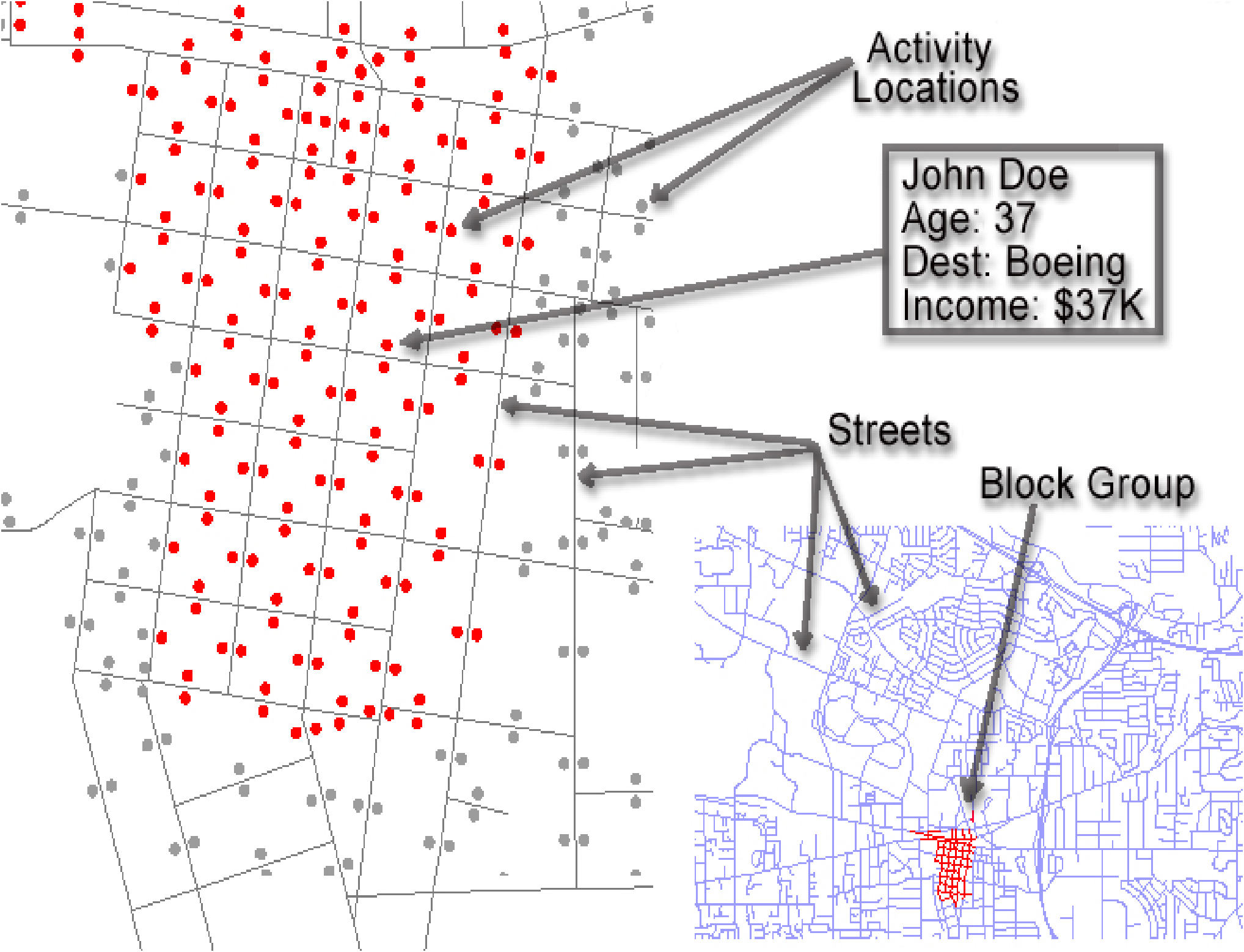
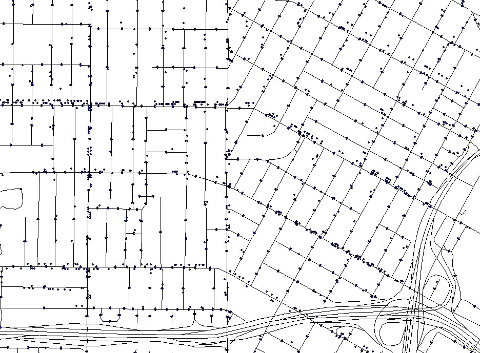
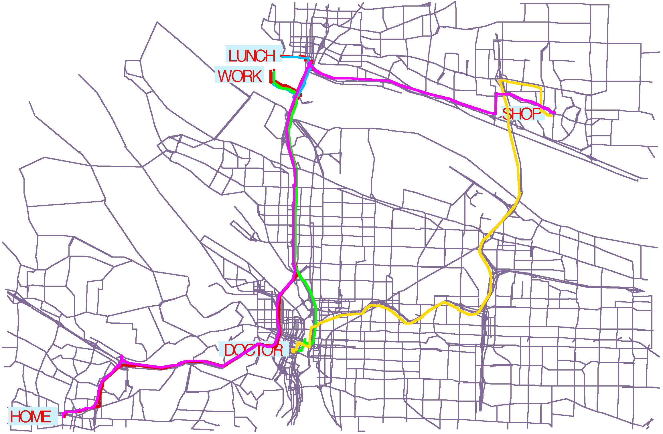
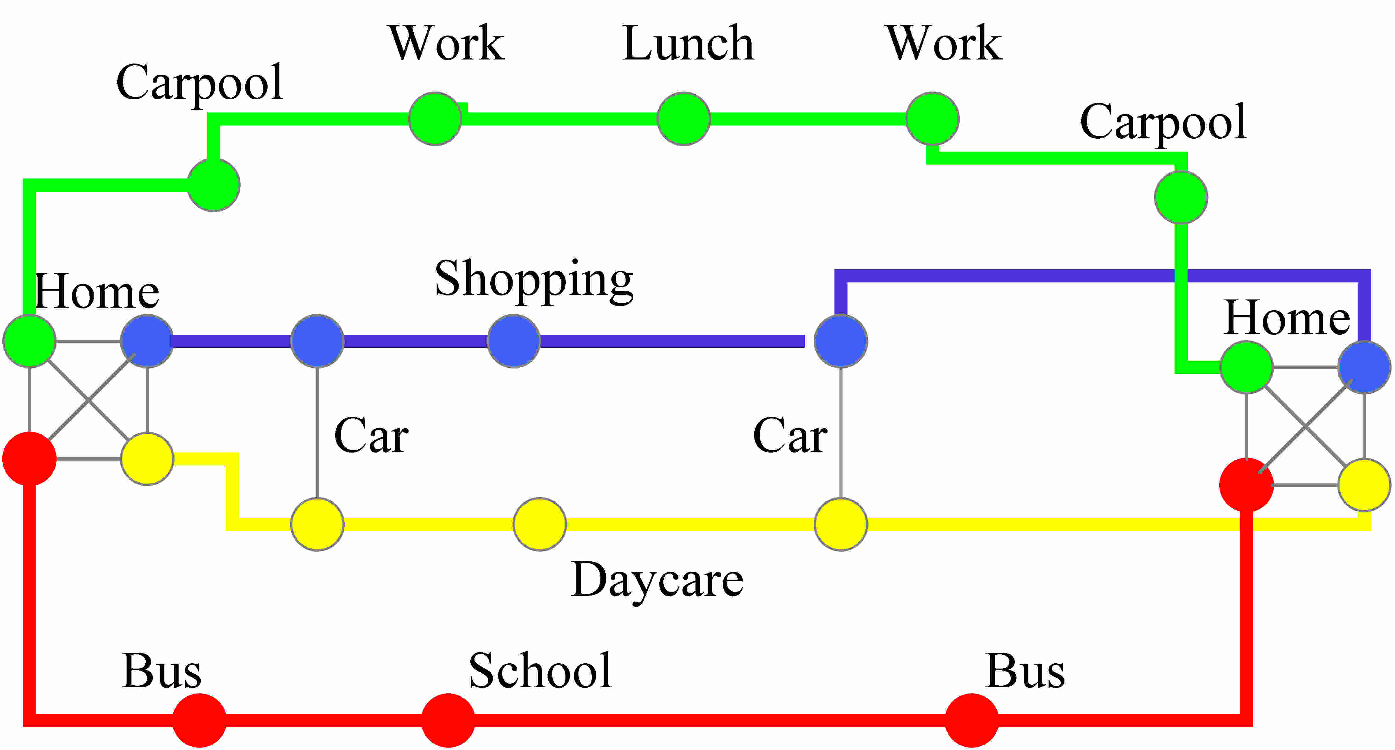
Figure 1. Households are geo-located to city half-blocks to match relevant demographic statistics in each of 12,226 block groups (top left). Business locations are geo-located by their business address (top right). Each individual is assigned an activity schedule (bottom left). Activity patterns are drawn from actual household activity surveys (bottom right)

Sublocation Modeling: How people interact at a location

2.12

EpiSimS partitions each location into sublocations, which are intended to represent individual classroom mixing groups within a school location, shops within a shopping center, or workgroups within a business location. Disease transmission only occurs between individuals who are in the same sublocation at the same time. The number of sublocations at each location is computed by dividing the location's peak occupancy by the appropriate mixing group size.

2.13

The mean workgroup size varies by standard industry classification code. Two data sources were used to estimate the mean workgroup size by SIC code. (Yee 1999) conducted a survey to determine the average worker density in the workplace, quantified as workers per square feet, by SIC code. The U.S. Dept. of Energy's Energy Information Administration conducted an extensive survey of commercial building usage, including workers per building, floors per building, and enterprises per building, by SIC code (Michaels 2003). The mean workgroup size was computed as the average from the two data sources (normalizing the worker density data), and ranges from 3.1 for transportation workers to 25.4 for health service workers. The average over all types of work is 15.3 workers per workgroup. For the runs presented here, the average mixing group sizes are 8.5 at a school, 11.2 at a college or university, 4.4 at a shop, and 3.5 at a social recreation venue.

Disease Transmission Model

2.14

The probability that a susceptible individual becomes infected during an activity is computed by accumulating transmission probability per unit time of contact with each infectious sublocation co-occupant. The base transmissivity, T = 0.00912 transmissions per contact hour, characterizes contact between a fully susceptible adult and a fully infectious, symptomatic adult. This baseline infectiousness was determined by calibrating the simulated clinical attack rate. The transmissivity between pairs of individuals is T multiplied by a susceptibility multiplier and an infectiousness multiplier. The infectiousness multiplier depends on the disease stage, the treatment history, and the age of the infectious person. The susceptibility multiplier depends on the treatment history of the susceptible individual. Individuals under age 19 have an infectiousness multiplier of 2 relative to adults, i.e., 0.0182 transmissions per contact-hour. Subclinical manifestations have an additional infectiousness multiplier of 0.5. After two days of infectiousness, a 0.25 multiplier is applied to the infectiousness of the remainder of the illness. Following the non-infectious incubation stage, there is a 12-hour infectious but non-symptomatic stage in which an infected person is 15% as infectious as they will be at their peak infectiousness.

2.15

If susceptible person j has a susceptibility multiplier S_j, and infectious person i has an infectiousness multiplier I_i, then the probability that susceptible individual j gets infected during an activity is computed as

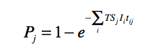
where t_ij is the time that susceptible person j was in the same sublocation as infectious person i, and the sum extends over all infectious persons that co-occupied the sublocation with individual j. EpiSimS computes the co-occupation times for all overlapping pairs of individuals as they enter and leave sublocations.

Influenza Disease Progression

2.16

Disease progression is characterized by 14 states. A susceptible individual (state 1) that becomes infected progresses through a sequence of disease states, beginning with non-infectious incubation (state 2) followed by a pre-symptomatic infectious stage (state 3). From there, an individual can become symptomatic-infectious (state 4), or asymptomatic-infectious (state 5a). The asymptomatic-infectious passes through a less-infectious stage (state 6a) and then recovers (state 8a). The symptomatic-infectious splits into two levels of severity: some continue their activities (state 5b), some stay home (state 5c). Those that continue their activities pass through a less-infectious stage (state 6b) on their way to recovery. Those symptomatics that stay home split into manifestations with (state 6d) and without (state 6c) severe complications such as pneumonia that would require hospitalization. Non-circulating symptomatics will either die (state 8b) or progress through a convalescent stage (state 7) on their way to recovery. The duration of each state is stochastic variable, with distributions of sojourn times matched to case history distributions (Longini 2004). Figure 2 shows the EpiSimS pandemic flu disease progression model.

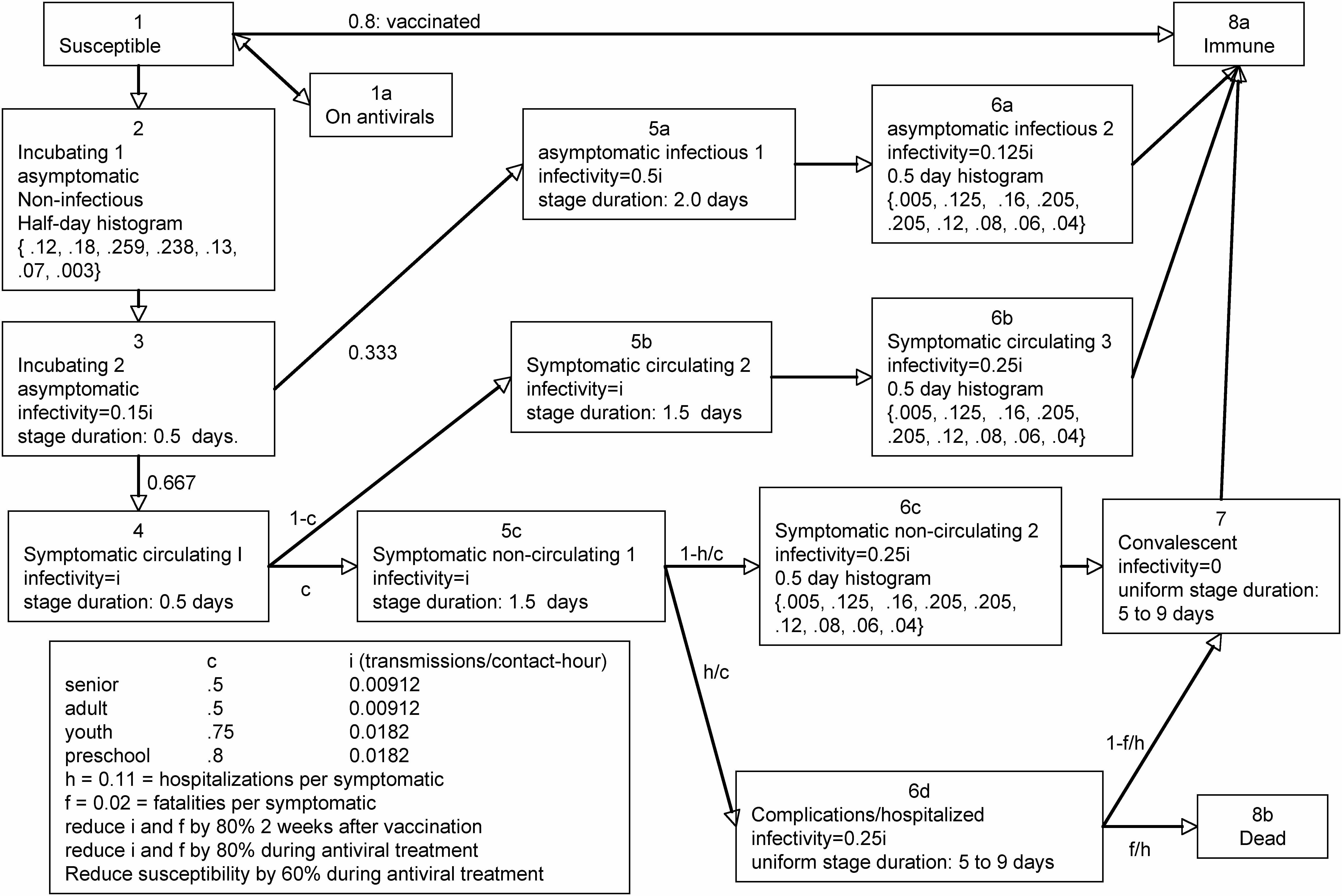
Figure 2. The pandemic influenza disease progression model. Each individual is initially in the uninfected stage. Upon becoming infected, all untreated individuals transition to the incubating-1 stage (pre-symptomatic incubating)

2.17

The incubation period of epidemic influenza ranges from one to three days (Longini 2004). The EpiSimS incubation-stage duration histogram is formulated with the half-day histogram {0, 0.12, 0.18, 0.259, 0.238, 0.13, 0.07, 0.003}, giving respectively the fraction of cases that incubate for a period of between 0 and 0.5 days, 0.5 and 1.0 days, etc. before transitioning to the infectious stage. This half-day histogram gives an averaged incubation stage duration of 1.9 days. The last 12 hours of this incubation stage is taken to be 15% as infectious as the following fully-infections stage.

2.18

The average infectious stage duration is 4.1 days (Longini 2004). The EpiSimS ill-stage duration histogram is formulated with a half-day histogram {0, 0, 0, 0, 0.005, 0.125, 0.16, 0.205, 0.205, 0.12, 0.08, 0.06, 0.04}, giving the fraction of illnesses that last for 0 to 0.5 days, 0.5 to 1.0 days, etc. The first two days of this stage are taken to be fully infectious, and any remaining time in this stage is one-quarter as infectious (Glass 2006).

2.19

EpiSimS models that 1/3 of infections are subclinical, and 2/3 are symptomatic (Longini 2004). Subclinical cases are taken to be half as infectious as cases that exhibit symptoms (i.e. 0.00456 transmissions per contact-hour for sub-clinical adults and seniors, 0.00912 for sub-clinical children). Their incubation and infectious stage durations follow the same histograms as those cases that do exhibit symptoms. Individuals with subclinical manifestations continue their normal activities during their "illness".

2.20

EpiSimS models that 50% of adults and seniors, 75% of students, and 80% of preschoolers will stay at home within 12 hours of the onset of influenza symptoms (Halloran 2002). Once these individuals stop their normal activity pattern, they can transmit disease only to household members or visitors. The EpiSimS pandemic influenza model assumes a case fatality rate of 2%, independent of age, and that 11% of symptomatics will be hospitalized if a bed is available (USDHHS 2005).

Implementation of the EpiSimS Simulation

2.21

EpiSimS is implemented as a set of C++ classes. The core EpiSimS package, EPI, contains the classes used to set up and run a simulation, and to represent the entities involved. It consists of 31,704 lines of C++ code in 65 header files and 62 source code files. In addition, several packages contain classes used to manage the multiple processors (MPIToolbox), serialization needed for restart capability (SERIAL), an indexing scheme that allows large amounts of data to be held in multiple files that are accessed as though they were in a single file (INDEX), input and output (EIO), and simulation control (CONTROLLER). The EpiSimS simulation requires current installations of several common utilities and libraries (boost, db, mpich, openmpi, libtool).

2.22

An EpiSimS user executes the qsub utility to acquire a set of processors from the cluster. One processor node is designated as the master, and the others are designated as slaves. A copy of the executable code is loaded on each processor, and the main process is started on each processor. The code contains branch statements so that different code can be executed on the master and slave processors. The main method is in the EpiSim class. It instantiates an ESimulator object and a local event queue. The ESimulator sets up and executes the distributed simulation according to the following pseudocode:

ESimulator::main
    Initialize local parameters from the config file 
    Register to receive messages from other processors
    Create and open a local event logger 
    Read in the disease manifestation (parameters giving fig. 2)
    IF master 
        Read in the partition file (sublocations per location)
        Read in disease states (initial health of each person)
        Send each location to the appropriate processor.
        Read in schedule file (activities for each person)
        Send each individual to the appropriate processor.
        Until endOfSimulation 
            receive and log results 
    ELSE
        Receive locations
        Receive individuals
        Place scheduled events on event queue
        Until endOfSimulation
            Handle next event

2.23

A simulation run requires several input data files and a user-specified configuration file that controls an individual scenario. The population file contains one record for each individual in the synthetic population. An example record is:

    101 1 52 1 1 603389 24177686 202000 24177686

This record parses as: Person 101 resides in household 1, is a 52 year old, male, worker. His household is located on city half-block 603389, which is on NAVTEQ road segment 24,177,686. His household income is $202,000. He begins the simulation at his home location.

2.24

The schedule file contains the daily activities for each person. Each record specifies a time, place, person, event type, and activity type. The schedule file records for person 101 are:

00:00:00 24177686 101 5 0
08:15:00 24177686 101 1 23914209
08:45:00 23914209 101 0 1
18:30:00 23914209 101 1 24177686
18:49:59 24177686 101 0 0
21:19:59 24177686 101 1 23937362
21:28:59 23937362 101 0 6
21:30:00 23937362 101 1 24177686
21:45:00 24177686 101 0 0

The first field specifies the time (HH:MM:SS). The second field gives the road segment where the activity occurs. The third field specifies the person. Values for the 4^th field specify the event type: 5-activity at start of simulation; 1- depart from activity; 0- arrive at activity. For departure events, the 5^th field gives the location of the next event. For start-simulation and arrival events, the 5^th field specifies the activity type: 0-home; 1-work; 2-shop; 3-visit; 4-social recreation; 5-other -an activity category allowed on the NHTS survey; 6-car pool; 7-school; 8-college.

2.26

The behavior of individuals is represented by their chain of events rather than by methods associated with the EPerson class. The disease-relevant interactions between individuals are computed entirely from the time they spend together in a sublocation. This contact time, along with a probability-based determination of whether a given contact causes a disease transmission, is computed by the method SpreadDisease. SpreadDisease is called by the ERoom object representing each sublocation whenever a person leaves that sublocation. The SpreadDisease algorithm is illustrated by the following pseudocode:

EDiseaseTransmitter::SpreadDisease
    GET list of room occupants and time since last update
    Instantiate working variables
    FOR each pair of room occupants
        Increment their contact time
    Make empty lists of infectious and susceptible people
    FOR each person in list of room occupants
        infectivity = GetInfectivity of person
            IF (infectivity > 0) add person to list of infectiousPersons;
            susceptibility = GetSusceptibility of person
            IF (susceptibility > 0) add person to list of susceptiblePersons
            IF (person is CurrentlyExposed) THEN
            add person to list of exposedPersons
            ELSE add person to list of unexposedPersons
    END FOR
    IF no one in room is infectious
        MARK every person in room as unexposed
        return
    MARK every person in room as exposed
    IF no one in room is susceptible THEN return
    FOR each susceptible person in room
        susceptibility = GetSusceptibility of susceptiblePerson
        IF susceptiblePerson is wearing a mask, reduce susceptiblity
        sumOfLogs = 0
        FOR all infectious persons in room
            infectivity = GetInfectivity of infectiousPerson
            reduce infectivity if infectiousPerson is wearing mask
            spreadability = susceptibility * infectivity 
                            * seasonalVarFactor * TransmissionFactor
            sumOfLogs += Math.log(1 - spreadability)
        END FOR
        prob=(1.-exp(deltaTMinutes * sumOfLogs)) 
        rannum <- random uniform variate in (0,1)
        if (rannum < prob) then susceptableperson becomes infected
    end for

2.27

The EpiSimS simulation environment has been ported to the LANL institutional computing cluster, Coyote. Coyote is a large HPC Linux cluster with an architecture comprised of 1290 nodes (2 AMD opteron processors at 2.6 GHz per node), using Voltaire InfiniBand interconnect, with 10.2 TeraBytes of RAM, sharing 50 TB Panasas disk storage with other clusters. Two or three 360-day EpiSimS simulations can be run in an overnight batch.

Social Contact Structure Results

3.1

The social contact network emerges as individuals move through their daily activities and come into and out of contact at sublocations. This section describes some characteristics of the emergent social contact network that only become visible when massive simulation is combined with demographic data, business directory data, and household activity surveys. Prior to any behavior changes related to the pandemic, 212 million contacts occur daily, each representing the physical proximity of two individuals. On average, each individual has 22.55 contacts per day. The average contact duration is 2.73 hours. On average, each individual has 61.54 contact hours per day.

3.2

Figure 3 shows the resulting degree distribution of the social contact structure, showing how many individuals have a given number of contacts in a typical day. The number of contacts a person has each day ranges from 1 to 153. Neither simple contact structure models (as in fully mixed contact groups of specified size) nor analytic contact structure models (as in power-law distributions) capture the distribution seen in the emergent social contact structure.

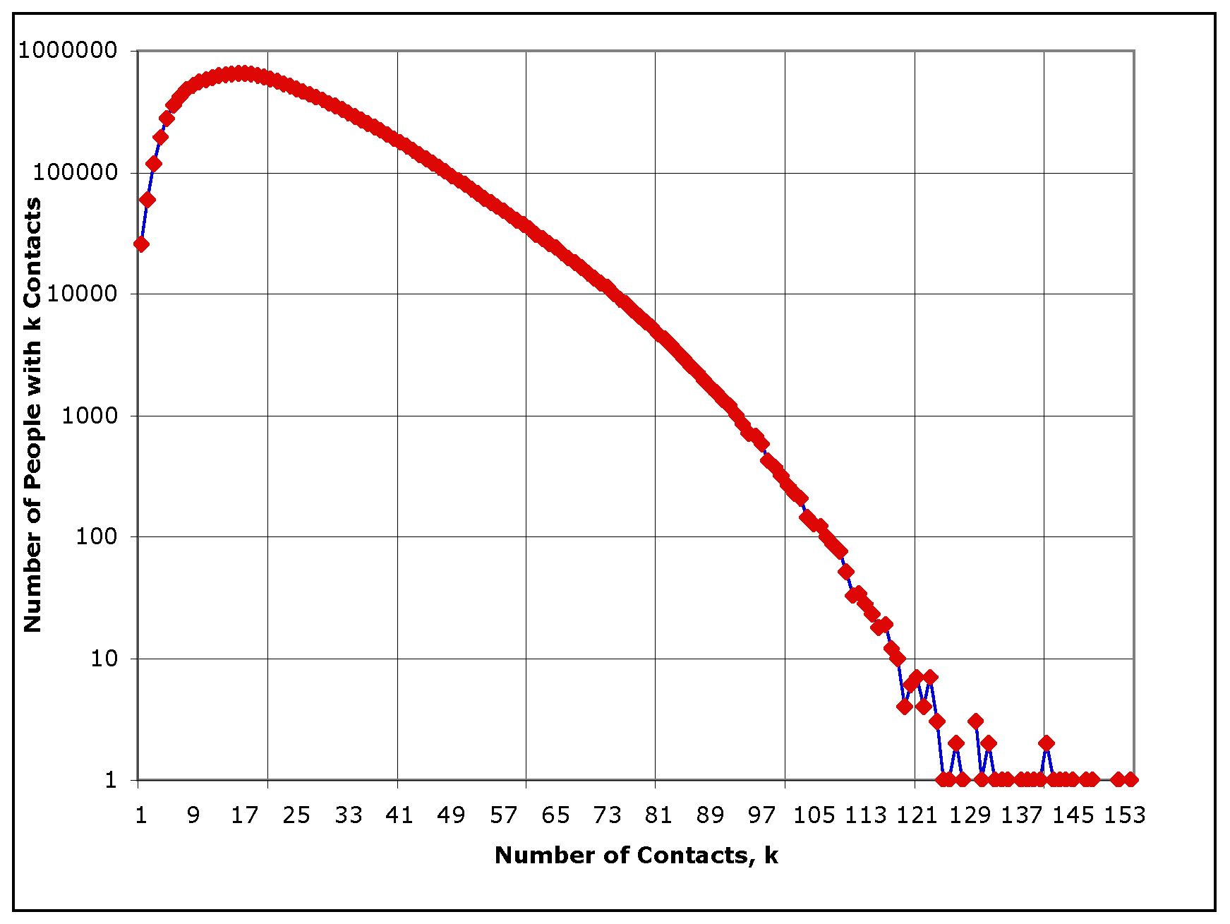
Figure 3. The degree distribution, showing how many people have a given number of contacts per day, for the synthetic population of southern California

3.3

Figure 4 shows the distribution of contact durations that emerges from massive simulation of individuals arriving at and departing from millions of locations. There are many short-duration contacts: roughly 2/3 of contacts last less than 2 hours and these appear to follow an exponential rather than a Poisson distribution.

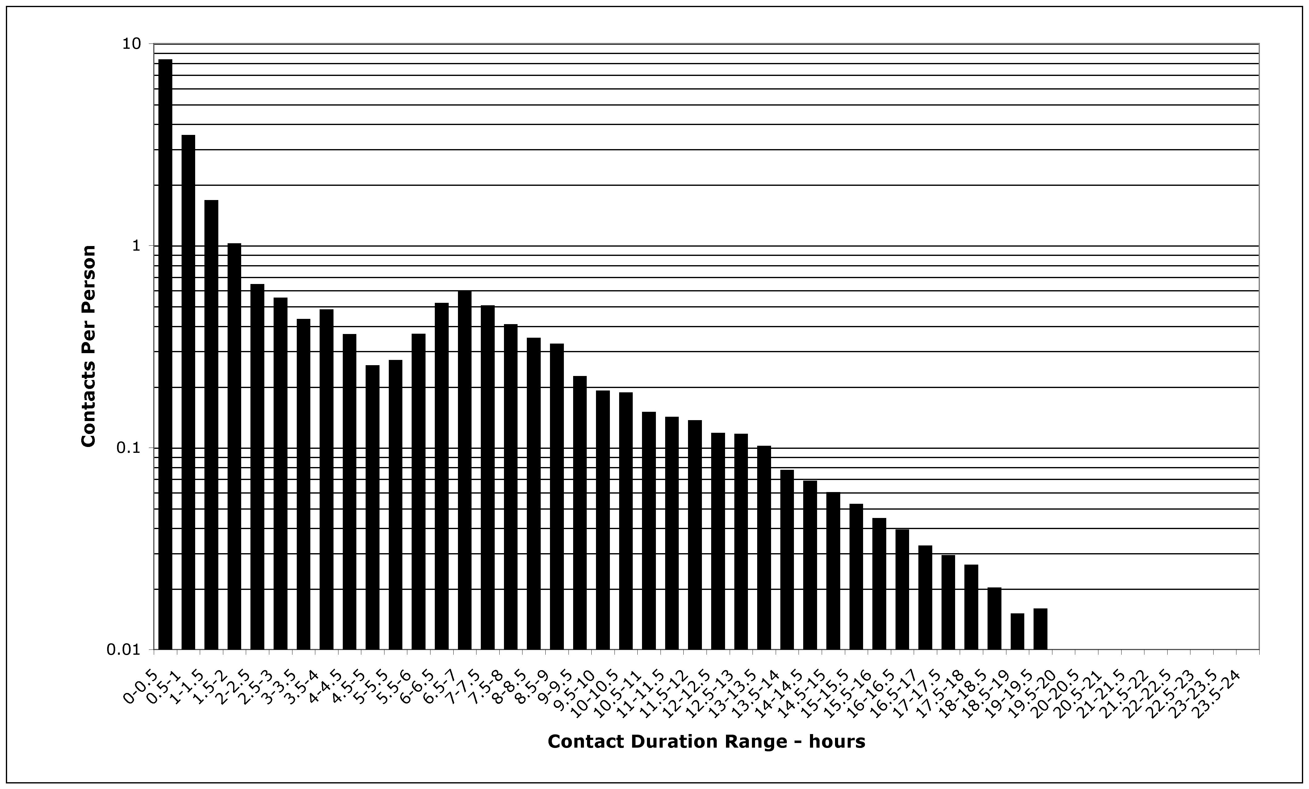
Figure 4. The distribution of contact duration among people in southern California

3.4

Figure 5 shows the distributions of contact durations in each of the EpiSimS activity categories.

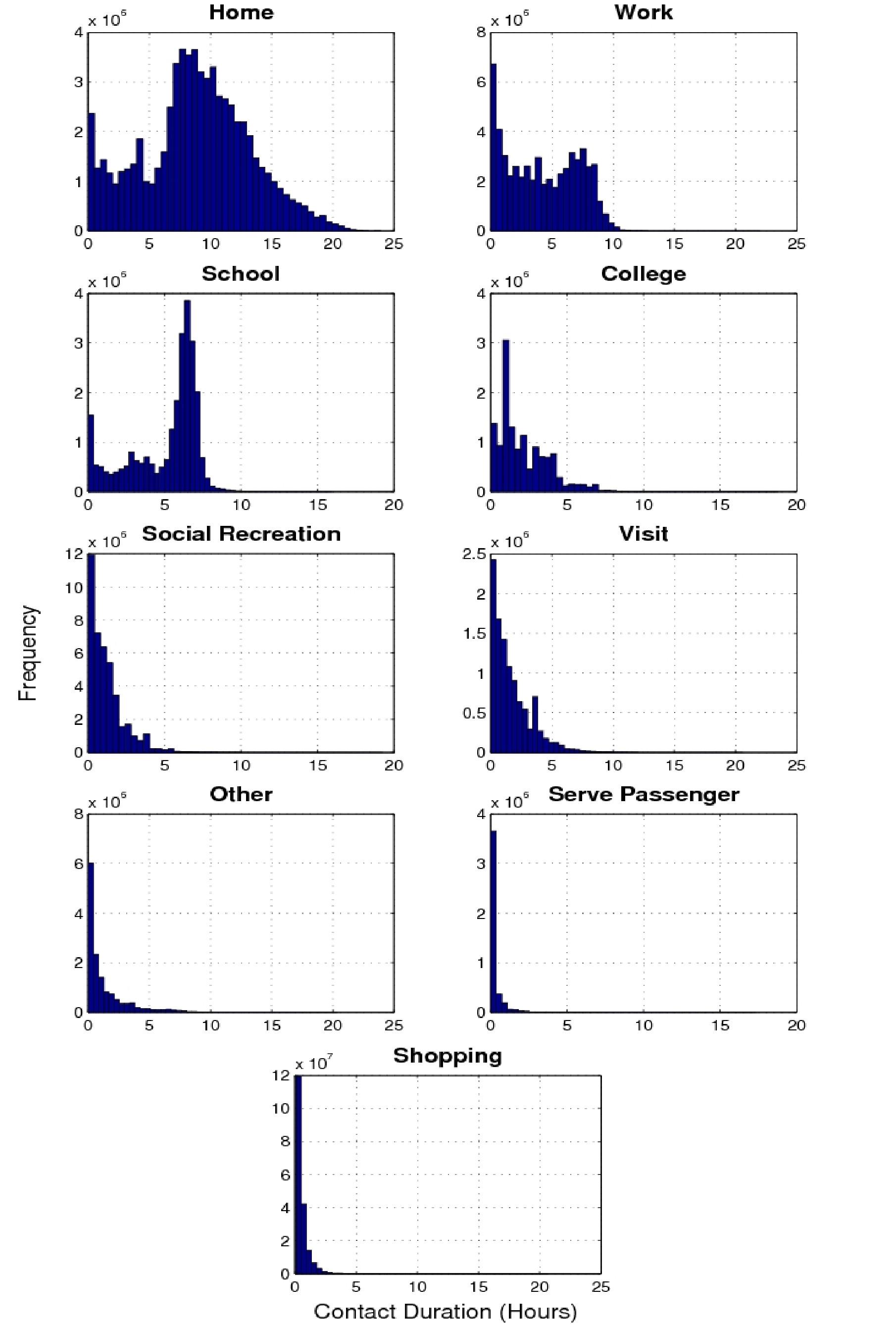
Figure 5. The distribution of contact duration for each activity type

3.5

Table 2 shows the average contact duration by activity category. The longest contacts occur at home, with an average contact duration of almost 9 hours, followed by school and work with an average duration of contact of 5.0 and 4.2 hours, respectively.

Table 2: Average duration per contact by activity category
Activity category	Average Duration	Standard Deviation
Home	8 hrs 49 min	4 hrs 28 min
School	5 hrs 2 min	2 hrs 14 min
Work	4 hrs 13 min	2 hrs 55 min
College	2 hrs 6 min	1 hr 40 min
Visit	1 hr 43 min	1 hr 39 min
Other	1 hr 19 min	1 hr 45 min
Social Recreation	1 hr 12 min	1 hr 14 min
Shop	30 min	55 min
Carpool	18 min	43 min

3.6

Fig. 6 shows the average daily contact hours per person, as a function of the person's age, for all contacts, and for household contacts. The average is 61.5 total contact-hours per person per day of which 30.9 occur at home.

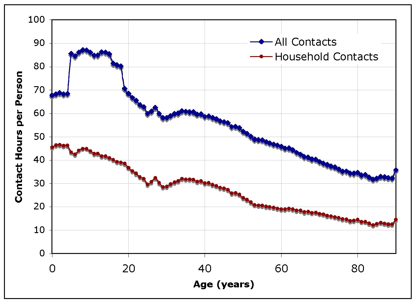
Figure 6. Average number of total and household contacts hours per person per representative day, as a function of the age of the person

3.7

Table 3 shows the average number of contact hours per person per day, by age group. Table 4 shows the average home-related contact hours per person per day.

Table 3: Daily average number of contact hours by age group
	average contact hours per day with preschoolers	average contact hours per day with students	average contact hours per day with adults	average contact hours per day with seniors
preschoolers (0-4)	15.03	16.84	34.52	1.92
students (5-18)	5.84	46.02	30.86	1.97
adults (19-65)	4.27	10.89	36.99	3.56
seniors (66+)	1.61	4.63	21.62	7.78

Table 4: Daily average number of home-related contact hours by age group
	average household contact hours per day with preschoolers	average household contact hours per day with students	average household contact hours per day with adults	average household contact hours per day with seniors
preschoolers (0-4)	7.21	12.45	25.68	0.69
students (5-18)	4.30	14.44	22.35	0.83
adults (19-65)	3.11	7.80	15.02	1.23
seniors (66+)	0.57	1.96	6.75	5.62

3.8

A worker has on average approximately 60 at-work contact-hours on a day he or she goes to work (an average of 14.3 work contacts averaging 4.2 hours each). Similarly, a student has on average approximately 38 at-school contact-hours on a day he or she goes to school (an average of 7.5 contacts, and 5.0 hours per contact).

Disease Spread Results

Temporal results: new infections per day

4.1

The percentages of the population that become infected each day, and that become symptomatic each day, are shown in Figure 7 for the 6-county southern California region. The pandemic is initiated by infecting 100 randomly selected individuals on day 0. Once the epidemic is established, there is a period of exponential growth, characterized by a growth rate of approximately 16% per day. After the peak of the pandemic passes, the new case rate drops exponentially, decreasing by about 14% per day. At the pandemic peak, about 10% of the population will be symptomatic or convalescing.

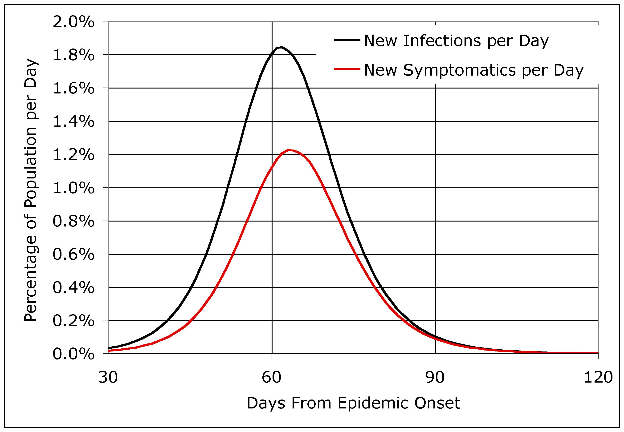
Figure 7. The base case EpiSimS simulation run, showing the percentage of the population that becomes infected or symptomatic per day

4.2

The peak new infection rate of approximately 347,000 new infections per day occurs 61.5 days after initiation of the epidemic. The peak new symptomatic rate occurs on day 63. The exact day on which these peaks occur varies over a few days from run to run, because of the stochastic nature of the early stage of the epidemic. At the peak, 1.84% of the population is becoming infected per day, and the cumulative number of cases reaches 4,346,480. By day 185, when there were no longer any infected people, 8,643,636 people had been infected. 45.9% of the population becomes infected and 30.6% of the population becomes symptomatic.

4.3

The average number of transmissions per infected person is known as the reproductive number, R. The reproductive number extracted from the simulation results is very well approximated by R=1.75 (S/P)^1.9, where S is the current number of susceptible individuals and P is the initial population (Stroud 2006).

Acquisition of Illness by Activity

4.4

EpiSimS keeps a record of the activity that each person was doing when he or she became infected. The breakout of cumulative infections by activity category for the whole epidemic is shown in Table 5.

Table 5: Breakout of infections by activity category
Activity category	Fraction of cumulative infections
Home	58.4%
School	13.3%
Work	13.0%
Shopping	5.5%
Social Recreation	3.6%
Visit	3.0%
College	1.8%
Other	1.3%
Carpool	0.1%

4.5

Throughout the simulation over half of infections are acquired at home. The fraction of new infections that are acquired at home rises from around 50% at the beginning of the epidemic to around 65% as the epidemic is winding down. The percentage of infections acquired at school drops from 25% down to only 3% at the end of the pandemic. The percentage of infections acquired at work increases from 10% to 15%.

Age dependence of infections

4.6

Figure 8 shows the overall attack rate for each age cohort, counting both clinical and asymptomatic cases. The clinical attack rates by age group are: preschoolers 28.1%, students 44.3%, adults 27.0%, and seniors 15.9%. Students suffer the highest attack rate, which is consistent with historical data (Simonsen 1998). Middle-aged adults suffer a high attack rate due to the interactions they have with their children, who serve as a path of spread among families and neighborhoods.

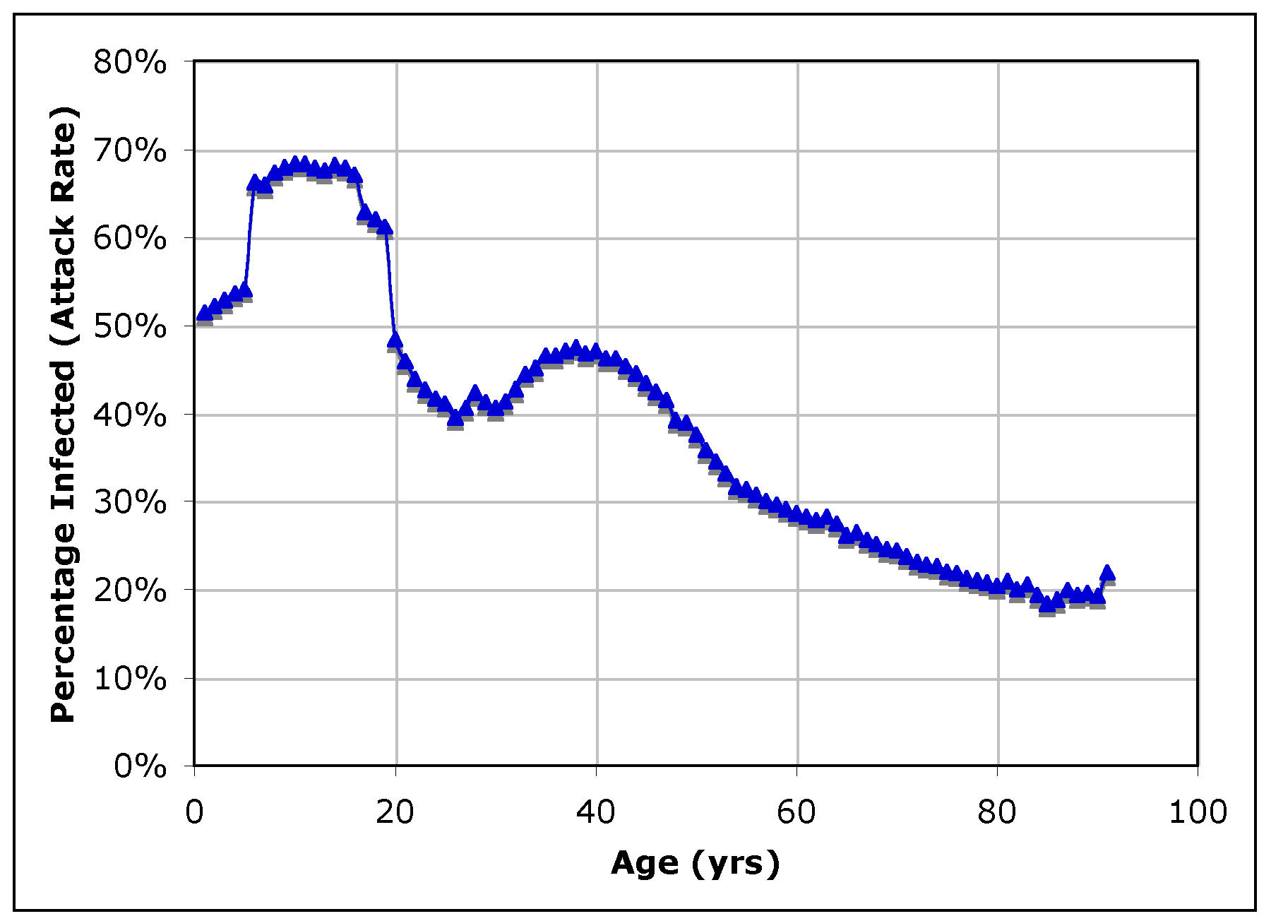
Figure 8. Total attack rate (symptomatic and subclinical) by age cohort

Spatial Hotspots and Correlation with Local Demographics

4.7

The new symptomatic cases occurring in the synthetic households were aggregated to obtain the clinical attack rate for each of the 3978 census tracts in southern California. The clinical attack rate by tract ranges from 9% to 56%, with a mean of 30.6% and a standard deviation of 7.5%. The clinical attack rate computed by the EpiSimS simulation shows obvious spatial clustering. Figure 9 indicates the clinical attack rate in each census tract. Clear sub-county hotspots are apparent.

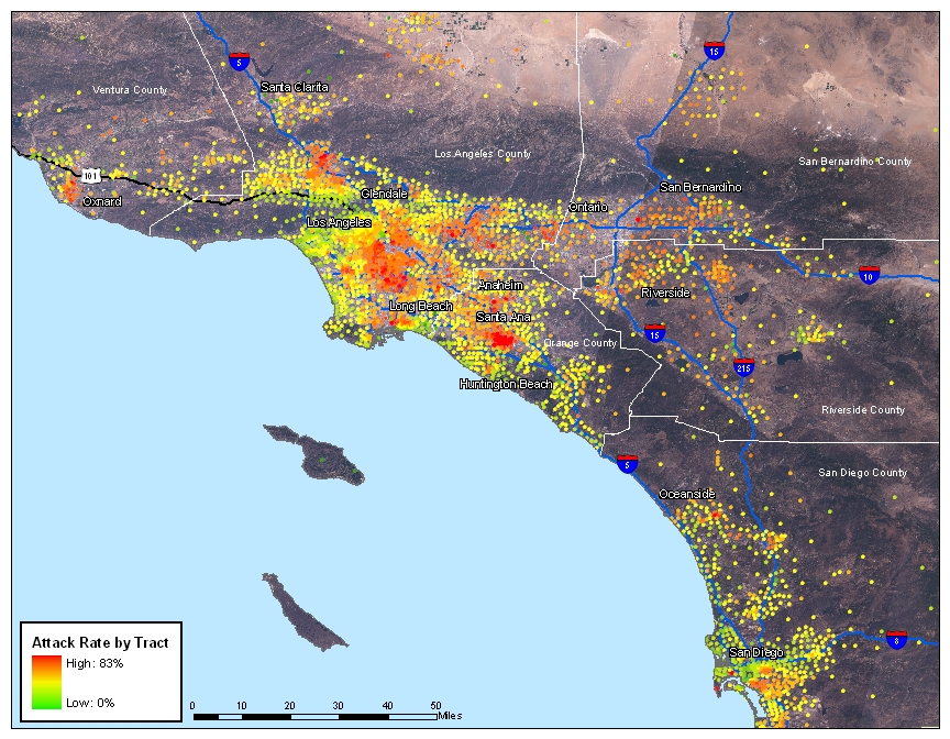
Figure 9. Clinical attack rate by census tract, ranging from mild (green) to severe (red)

4.8

The worst hot-spot in the simulation is seen in synthetic Santa Ana, where the 185,604 household residents of 28 contiguous severely-hit census tracts suffer a 52% clinical attack rate, exceeding the southern California average by 75%. The pandemic peaks five days earlier in this hot-spot than in Southern California as a whole. Santa Ana has the highest average household size of any major US city.

4.9

Three major hot-spots of 55,000 to 85,000 residents are seen in synthetic South Los Angeles, Compton/Lynwood, and Pacoima. Seven smaller hot-spots (10,000 to 25,000 residents) occur in synthetic Anaheim, El Monte, Long Beach, Oxnard, Pomona, South San Jose Hills, and Watts.

4.10

The clinical attack rate by census tract was analyzed for correlations with demographic characteristics of the census tracts. The strongest correlation was found with the average household size. Significant correlation was found with per capita income, and with the student fraction of the population. Mild correlation was found to population density. No correlation was found between clinical attack rate in a tract and the population of the tract.

4.11

Figure 10 shows the simulated clinical attack rate plotted against the average household size, for each of the 3978 census tracts in southern California. 90% of the variation in clinical attack rate by census tract can be attributed to correlation between clinical attack rate and average household size.

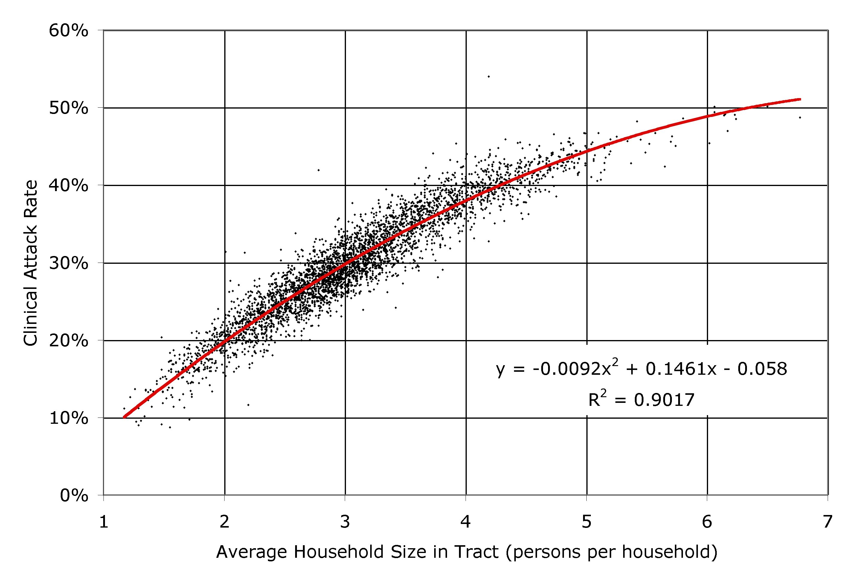
Figure 10. The clinical attack rate plotted against the average household size (i.e. the residential population divided by the number of households) for each of the 3978 census tracts in southern California, as simulated by EpiSimS

4.12

Figure 11 shows the clinical attack rate plotted against the percentage of the population that is of student age, for each of the 3978 census tracts in southern California. 69% of the variation in clinical attack rate by census tract can be attributed to correlation of clinical attack rate and the student percentage. A similar degree of correlation, but of the opposite sense, is seen when the tract clinical attack rate is viewed against the fraction of the population that is in the workforce.

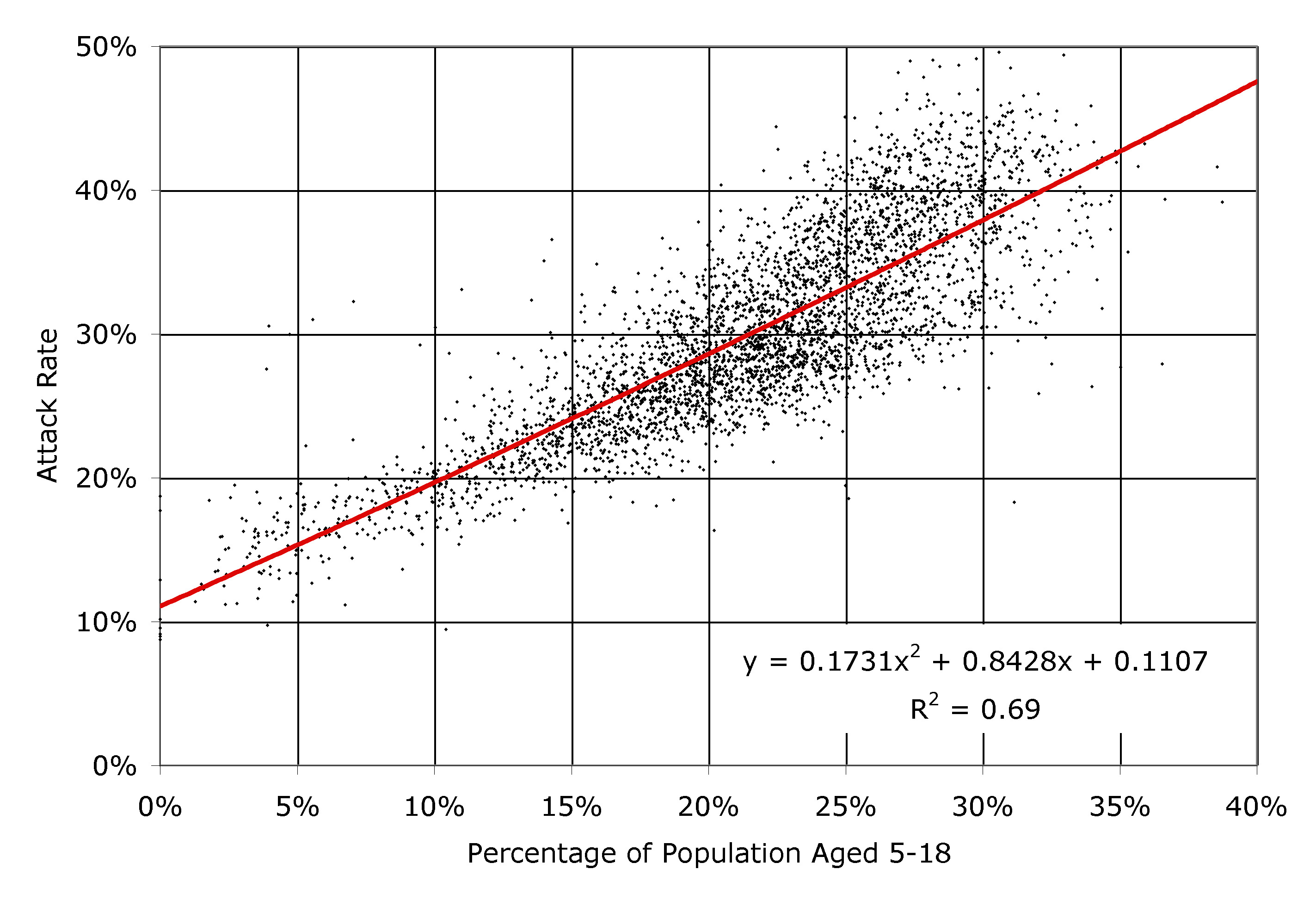
Figure 11. The clinical attack rate plotted against the ratio of students to non-students, for each of the 3978 census tracts in southern California, as simulated by EpiSimS

4.13

Figure 12 shows the clinical attack rate plotted against the base 10 logarithm of the per capita income, for each of the 3978 census tracts in southern California. The tract per capita incomes were taken from 1999. 58.6% of the variation in clinical attack rate by census tract can be attributed to correlation of clinical attack rate with per capita income.

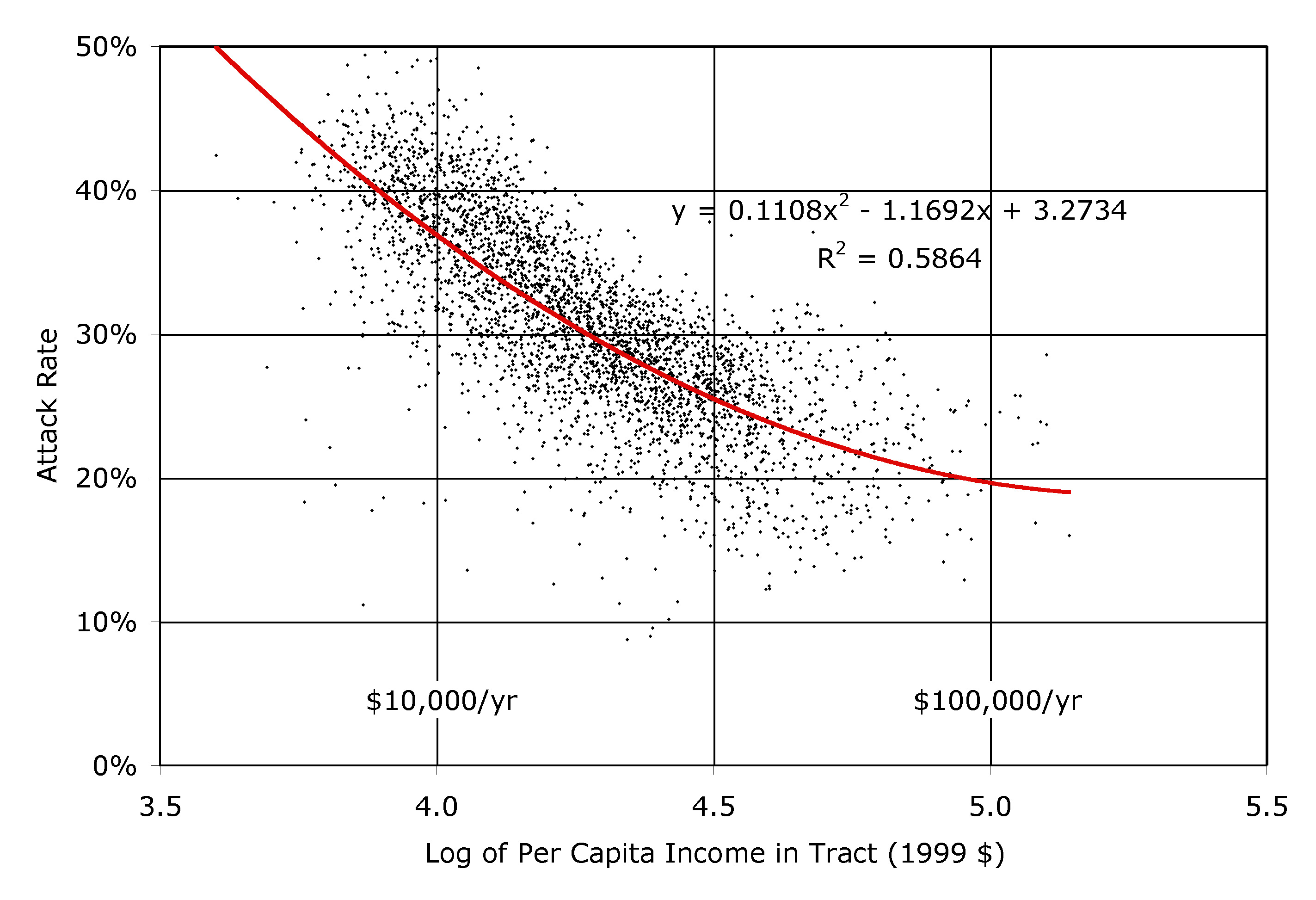
Figure 12. The clinical attack rate plotted against the logarithm of the per capita income, for each of the 3978 census tracts in southern California, as simulated by EpiSimS

4.14

Figure 13 shows the clinical attack rate plotted against the population density, for each of the 3978 census tracts in southern California. 13.3% of the variance in clinical attack rate by census tract can be attributed to correlation of clinical attack rate with population density. Roughly, each additional 1000 residents per square kilometer adds 1% to the expected attack rate in a census tract.

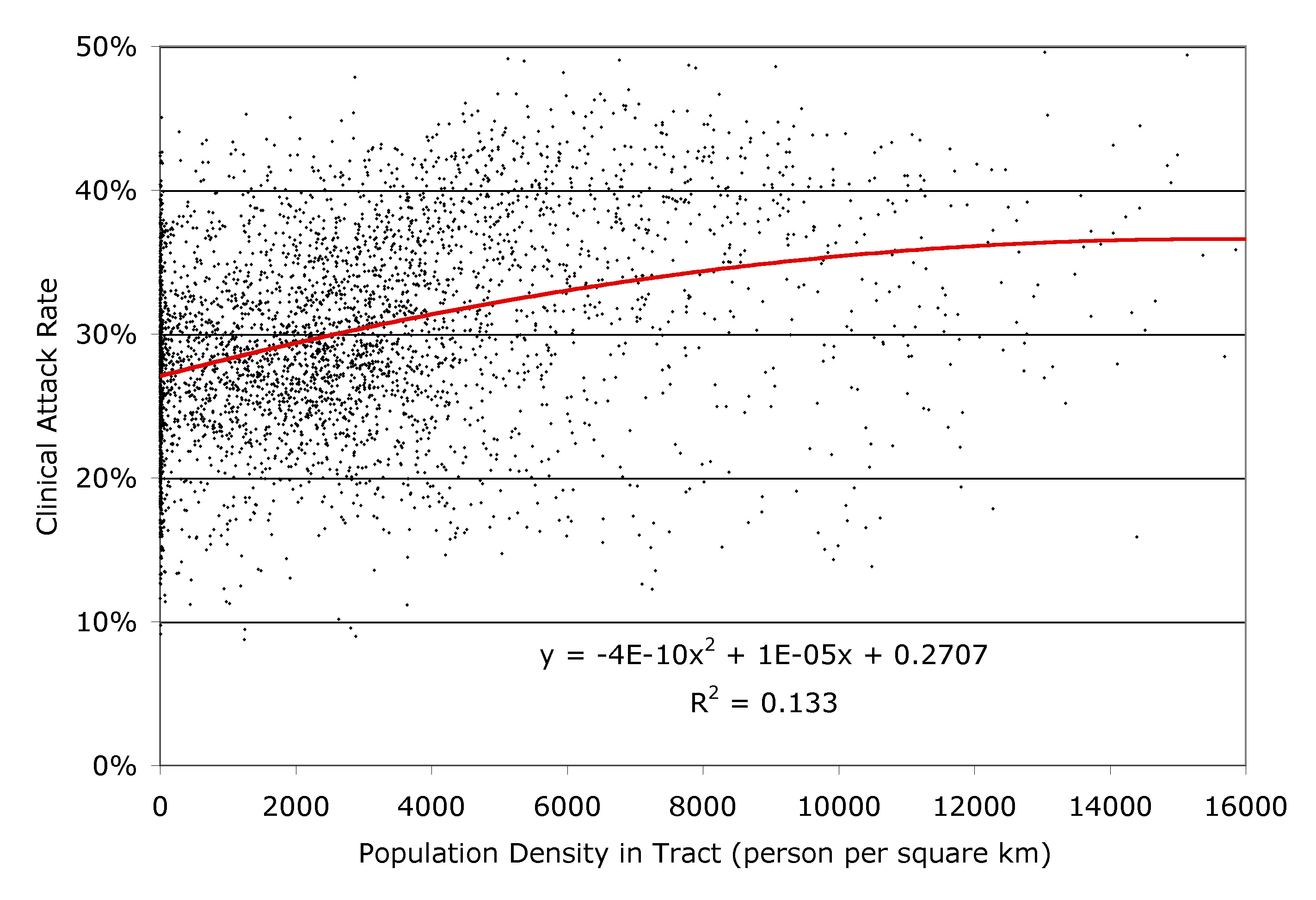
Figure 13. The clinical attack rate plotted against the population density, for each of the 3978 census tracts in southern California, as simulated by EpiSimS

Conclusion

5.1

The EpiSimS simulation is an attempt to compute the elusive dynamic social contact network, and the characteristics of disease spread on that network, making the best use of available data. 19 million individuals residing in 6 million households go about their daily activities at 2.3 million locations. The artificial society is constructed to match relevant demographics at census block group (~1500 person) granularity. Locations in the synthetic landscape are matched to actual businesses and road segments. Synthetic activities are drawn from activity schedules reported by actual households. Individuals are passive entities that are carried around the landscape by their activity schedules, but disease can modify behaviors by causing some activities to be skipped. EpiSimS provides a unique tool to generate the dynamic social contact network by tracking which individuals happen to be at the same place at the same time.

5.2

We find that the average household size of a community is a powerful predictor (Pearson's correlation coefficient of 0.9) of the local severity of an influenza pandemic. Because of strong correlations between average household size, per capita income, and fraction of population of student age, the predictive power of the latter two characteristics is essentially subsumed by that of the average household size. Like any model, EpiSimS incorporates many simplifications, approximations, and assumptions. Consequent to these assumptions, particularly those concerning the relative transmissivity of disease at home, the EpiSimS simulation finds that 58% of the infections in a simulated influenza pandemic are acquired at home. It is not too surprising, therefore, that places with larger average household size would tend to suffer higher pandemic attack rates.

5.3

Population density is a surprisingly poor predictor of simulated local pandemic severity. The assumed mixing group sizes do not depend very strongly on population density. The local clinical attack rate is essentially independent of the number of people residing in the community.

5.4

Caution must be used when generalizing model results to support planning decisions. Nevertheless, it is reasonable to expect that for a contagious disease in which many infections are acquired from household members, an outbreak, epidemic, or pandemic will be more severe in communities that have a relatively large average household size. Consideration of this correlation could improve the effectiveness of pandemic planning.

References

BARRETT C L, Eubank S G, Smith J P (2005) If Smallpox Strikes Portland, Scientific American 292, March 2005. pp. 41-49.

BECKMAN R J, Baggerly K A, and McKay M D (1995) Creating Synthetic Baseline Populations, Transportation Research A 30A(64). pp. 415-429.

DUNHAM J B (2005) An Agent-based Spatially Explicit Epidemiological Model in MASON, Journal of Artificial Societies and Social Simulation 9(1)3, https://www.jasss.org/9/1/3.html.

EIDELSON B, Lustik I (2004) 'VIR-POX: An Agent-based Analysis of Smallpox Preparedness and Response Policy', Journal of Artificial Societies and Social Simulation, 7(3)6. https://www.jasss.org/7/3/6.html

EUBANK S, Goclu H, Kumar A, Marathe M, Srinivasan A, Totoczkal Z, Wang N (2004) Modelling disease outbreaks in realistic urban social networks, Nature 429, 13 May 2004. pp. 180-184.

FHWA (FEDERAL HIGHWAY ADMINISTRATION) (1978) Quick-response Urban Travel Estimation Techniques and Transferable Parameters, NCHRP Report 187. available from http://nationalacademies.org/trb/bookstore

FERGUSON N M, Cummings D A T, Fraser C, Cajka J C, Cooley P C, Burke D S (2006) Strategies for mitigating an influenza pandemic, Nature 442(7101), July 27, 2006. pp. 448-452.

GERMANN T C, Kadau K, Longini I M, Macken C M (2006) Mitigation strategies for pandemic influenza in the United States, Proc. Natl. Acad. Sci. U.S.A. 103, pp. 5935-5940.

GLASS R J, Glass L M, Beyeler W E, Min H J (2006) Targeted Social Distancing Design for Pandemic Influenza, Emerging Infectious Diseases 12, Nov 2006.

HALLORAN M E, Longini I M, Nizam A, Yang Y (2002) Containing Bioterrorist Smallpox, Science 298, 15 November 2002. pp. 1428-1432.

HSC (HOMELAND SECURITY COUNCIL) (2006) National Strategy for Pandemic Influenza - Implementation Plan, http://www.whitehouse.gov/homeland/nspi_implementation_briefing.pdf.

HUANG C-Y, Sun C-T, Hsieh J-L, and Lin H (2004) Simulating SARS: Small-World Epidemiological Modeling and Public Health Policy Assessments, Journal of Artificial Societies and Social Simulation 7(4)2, https://www.jasss.org/7/4/2.html.

KRETZSCHMAR M, van den Hof S, Wallinga J, van Wijngaarden J (2004) Ring vaccination and smallpox control, Emerging Infectious Diseases 10. pp. 832-841.

LONGINI I M, Halloran M E, Nizam A, Yang Y (2004) Containing Pandemic Influenza with Antiviral Agents, Am. J. of Epidemiology, 159(7) April 1, 2004, pp. 623-633.

MARTIN W A, McGuckin N A (1998) Travel estimation techniques for urban planning, NCHRP Report 365. available from http://nationalacademies.org/trb/bookstore

MICHAELS J (2003) Commercial Buildings Energy Consumption Survey, http://www.eia.doe.gov/emeu/cbecs/cbecs2003/detailed_tables_2003/detailed_tables_2003.html

NAVTEQ (2004) US Road Network Data, obtained in 2004, http://www.navteq.com

NCES (NATIONAL CENTER FOR EDUCATION STATISTICS) (2006) Common Core of Data public school data 2004-2005 school year, and Private School Universe Survey data for the 2003-2004 school year, http://nces.ed.gov/datatools/.

SIMONSEN L, Clarke M J, Schonberger L B, Arden N H, Cox N J, Fukuda K (1998) Pandemic versus Epidemic Influenza Mortality: A Pattern of Changing Age Distribution, J. Infectious Diseases 178. pp. 53-60.

SMITH L, Beckman R, Anson D, Nagel K, Williams M (1995) TRANSIMS: Transportation analysis and simulation system, Compendium of Papers of 5th Nat'l Conf on Transportation Planning Methods Applications-Volume II, Transportation Research Board, Seattle, Washington, April 1995.

STROUD P D, Sydoriak S J, Riese J M, Smith J P, Mniszewski S M, Romero P R (2006) Semi-empirical Power-law Scaling of New Infection Rate to Model Epidemic Dynamics with Inhomogeneous Mixing, Mathematical Bioscicences 203, pp. 301-318.

USCB (UNITED STATES CENSUS BUREAU) (2000) 2000 Decennial Census, database server at http://factfinder.census.gov.

USDHHS (UNITED STATES DEPARTMENT OF HEALTH AND HUMAN SERVICES) (2005) HHS Pandemic Influenza Plan, html://www.hhs.gov/pandemicflu/plan/pdf/HHSPandemicInfluenzaPlan.pdf.

USDOT (UNITED STATES DEPARTMENT OF TRANSPORTATION) (2003) NHTS 2001 Highlights Report BTS03-05, Washington, DC., http://www.bts.gov/publications/highlights_of_the_2001_national_household_travel_survey/html/executive_summary.html.

USINS (UNITED STATES IMMIGRATION AND NATURALIZATION SERVICE) (2003) Estimates of the Unauthorized Immigrant Population Residing in the United States: 1990 to 2000, http://www.dhs.gov/xlibrary/assets/statistics/publications/Ill_Report_1211.pdf.

VIBOUD C, Bjornstad O N, Smith D L, Simonsen L, Miller M A, Grenfell BT (2006) Synchrony, Waves, and Spatial Heirarchies in the Spread of Influenza. Science 312, pp. 447-451.

VOORHEES A M (1956) A general theory of traffic movement. 1955 Proceedings, Institute of Traffic Engineers, New Haven, CT.

YEE D and Bradford J (1999) Employment Density Study, Canadian METRO Council Technical Report, April 6 1999.

Return to Contents of this issue

© Copyright Journal of Artificial Societies and Social Simulation, [2007]