
J. Gary Polhill, Dawn Parker, Daniel Brown and Volker Grimm (2008)
Using the ODD Protocol for Describing Three Agent-Based Social Simulation Models of Land-Use Change
Journal of Artificial Societies and Social Simulation
vol. 11, no. 2 3
<https://www.jasss.org/11/2/3.html>
For information about citing this article, click here
Received: 03-Aug-2007 Accepted: 18-Dec-2007 Published: 31-Mar-2008

 Abstract
Hercules himself must yield to ODDs
Henry VI part III, Act II Scene I
Is the author clear about the goals of the model? Are these goals appropriate? Has the model appropriately represented relevant spatial processes? Have standard techniques for verification and validation been used? Are the mechanisms of the model clearly communicated to the audience? Have the model mechanisms been appropriately verified? How does the model compare to other ongoing ABM/LUCC work?
|
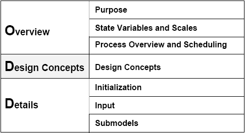
| Figure 1. The seven elements of the ODD protocol. The three categories on the left side are only for explaining the general structure of the protocol but are not used while describing a model. Rather, a model description following ODD has the seven sections listed on the right side. (After Grimm et al. 2006) |
Variable name | Brief description |
| Land Use | Main decision variable for the agent. Two types: zero (fixed price) or one (quantity-dependent price). |
| Coordinates | X and Y coordinates of the cell over which the land owner decides land use. |
Landscape model:
| Variable name | Brief description | Parameter in SLUDGE GUI |
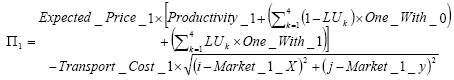
| Productivity | Per-cell land-use specific output variable. | Productivity_0 Productivity_1 |
| Externalities | Positive or negative Productivity change with each neighbouring Land Use (4 variables). These result in a gain or loss of production for the first Land Use when it shares a border with the second. | One_With_0 One_With_1 Zero_With_0 Zero_With_1 |
| Output Price 0 | Parametric output price for output of Land Use 0. | Output_Price_0 |
| Landscape dimension | Height and width of the model Landscape, in cells | Board_Size |
| Coordinates | X and Y coordinates of the cell, which determine transportation costs to market locations. | |
Supply and Demand model:
| Variable name | Brief description | Parameter in SLUDGE GUI |
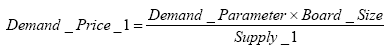
| Demand function | Downward-sloping function and scaling parameter that determines price of Output 1. | Demand_Parameter |
| Expected Price 1 | Price anticipated by each agent based on current Landscape and Economic Conditions. | |
| Output Price 1 | Realised price of Output 1 dependent on total output of Land use 1. | |
Transport cost model:
| Variable name | Brief description | Parameter in SLUDGE GUI |
| Coordinates | X and Y coordinates of the cell representing the market location for output of each Land use. | Market_0_X; Market_0_Y Market_1_X; Market_1_Y |
| Transport costs | Land-use specific per-unit transport cost. | Transport_Costs_0 Transport_Cost_1 |
|
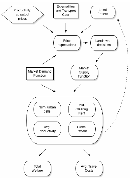
| Figure 2. SLUDGE process overview (ovals are endogenous/emergent elements; lateral boxes are exogenous/initialisation elements) |
Adaptation
Fitness
Prediction
Interaction
Sensing
Stochasticity
Observation
|
(1) |
|
(2) |
|
(3) |
|
(4) |
| Landscape Cells | |
| Variable name | Brief description |
| Coordinates | X and Y coordinates of the Cell, that determine the Euclidean Distance to Service Centres. |
| Aesthetic Quality | A relative indicator of the visual attractiveness of a Cell to the Residents. |
| Residents | |
| Name | Brief description |
| Coordinates | X and Y coordinates of the Cell where the Resident resides. |
| Alpha Aesthetic Quality* | Relative importance to resident of Aesthetic Quality. |
| Alpha Distance to Service Centres * | Relative importance to resident of Distance to Service Centres. |
| Alpha Neighbourhood Density * | Relative importance to Resident of Neighbourhood Density. |
| Alpha Neighbourhood Similarity * | Relative importance to Resident of Neighbourhood Similarity. |
| Utility | The overall level of satisfaction a Resident receives from a locational choice. |
| *All alpha values are constrained to sum to 1. | |
| Service Centres | |
| Variable name | Brief description |
| Coordinates | X and Y coordinates of the Cell where the Service Centre is located. |
For 1 to the defined number of Residents to enter at each time step (specified by the user or file)
	Create a new Resident.
	For 1 to the number of Cells to test
		Randomly select an unoccupied Cell (without replacement)
		Calculate Neighbourhood Similarity, based on the difference between the Resident's
			importance values for each locational attribute (α's) and those of any
			residents already located in the eight neighbouring cells.
		Evaluate Utility at that Cell to that Resident: based on the combination of Cell
			attributes, weighted by the importance of those attributes to the Resident
			(represented by alpha).
		If it is the first Cell then
			Store the Cell and Utility as the best location.
		Else if it is not the first Cell evaluated by the Resident then
			If the current Cell's Utility > best Cell's Utility then
				Set the best Cell and Utility to those of the current Cell
			End if
		End if
	Next Test Cell
	Put Resident in the best Cell.
	Set Resident X,Y and Utility to those from the new Cell
	Calculate Neighbourhood Density for all Cells, as the number of occupied cells within the
		nine-cell neighbourhood around each Cell.
	If option is selected, update Aesthetic Quality near new Resident

	If the total number of Residents in the world divided by the specified number of Residents per
		Service Centre minus the number of existing Service Centres is >= 1 then
		Create and locate a new Service Centre (process described in details)
		Set Service Centre X,Y properties to those from the new Cell
		Calculate Distance to Service Centres for all Cells, based on Euclidean distance from
			each Cell to the nearest Service Centre
		If option is selected, update Aesthetic Quality near new Service Centre
	End IF
Next Resident
Adaptation
Fitness
Prediction
Interaction
Sensing
Stochasticity
Collectives
Observation
|
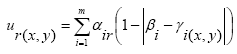
(5) |
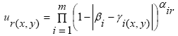
where ur(x, y) is the utility of location (x, y) for resident r; αir is the weight the resident r places on factor i; βi is the preferred value on component i and is usually assumed constant for all residents, e.g., all residents desire the most aesthetic quality and shortest distance to service centers; γi(x, y) is the value of component i at location (x, y), and m is the number of location attributes evaluated. The form of the multiplicative function is:
|
(6) |
Choice of whether to use the additive or multiplicative utility function is driven by theoretical and experimental considerations (Brown and Robinson 2006).
	Select a random adjacent Cell next to the last Resident
	Do until a Cell is selected for the Service Centre
		To get a new Cell spiral outwards from the last Resident Location, while
			checking for edge effects
		If the Cell is not occupied then
			 Select the Cell.
		End if
	End Do
| Land Parcel: Field scale | |
| Variable name | Brief description |
| Environment | The Environment this Land Parcel appears in (see below). |
| Biophysical Characteristics | An abstract representation of the local properties of the Land Parcel, which could conceptually be understood as such things as soil type, aspect, altitude or slope, though these are not specifically represented. |
| Land Use | An abstract representation of the land use this field has been applied to. |
| Yield | The Yield of the most recently applied Land Use. |
| Owner | The Land Manager responsible for making decisions for the Parcel, and harvesting the Yield from it. |
| Environment: Catchment or regional scale | |
| Variable name | Brief description |
| Spatial Topology | Determines the neighbourhood of each Land Parcel (toroidal/bounded; von Neumann/Moore). |
| External Conditions | An abstract representation of spatially homogeneous conditions that change over time and affect Economic Returns to Land Managers. These could be thought of as including such things as exchange rates, regional climate, and demand, though such things are not specifically modelled. |
| External Conditions Flip Probability Array | Probabilities determining the rate of change of the External Conditions from one Year to the next. |
| Biophysical Characteristics Clumped? | Whether or not to make the Biophysical Characteristics of neighbouring Land Parcels more similar to each other using a clumping algorithm. |
| Break-Even Threshold | The amount of Yield a Land Manager has to make from a Land Parcel to break even. |
| Land Uses | The set of Land Uses that Land Managers may apply to Land Parcels. |
| Land Manager: Farm scale | |
| Variable name | Brief description |
| Land Parcel List | List of Land Parcels owned by the Land Manager. |
| Subpopulation | The Subpopulation this Land Manager belongs to, which determines the settings of its parameters. |
| Land Market | A pointer to the Land Market to which bids for Land Parcels should be sent. |
| Account | The accumulated wealth of the Land Manager. |
| Aspiration Threshold | The amount of Yield the Land Manager hopes to obtain from each Land Parcel. |
| Imitative Strategy | The algorithm to use for choosing a Land Use by imitating neighbouring Land Uses if the Aspiration Threshold is not achieved. |
| Memory size | How many Years in the past the Land Manager may look for data in the Imitative Strategy algorithm. |
| Innovative Strategy | The algorithm to use for choosing a Land Use without imitating neighbouring Land Uses if the Aspiration Threshold is not achieved. |
| Imitation Probability | The probability of choosing the Imitative Strategy if the Aspiration Threshold is not achieved. |
| Land Offer Threshold | The amount that must be in the Account before the Land Manager will bid for Land Parcels. |
| Bidding Strategy | The algorithm to use to generate a Price to offer for Land Parcels available for sale. |
| Selection Strategy | The algorithm to use to decide which bids for Land Parcels to actually make. |
| Subpopulation: Land Manager collective | |
| Variable name | Brief description |
| Land Manager List | List of Land Managers belonging to this Subpopulation. |
| Incomer Offer Price Distribution | Determines the distribution from which new Land Managers of this Subpopulation will create an offer price for Land Parcels — e.g. Normal(Mean, Variance). |
| Imitative Probability Distribution | Distribution from which the Imitative Probabilities of new Land Managers of this Subpopulation are taken. |
| Aspiration Threshold Distribution | Distribution from which the Aspiration Thresholds of new Land Managers of this Subpopulation are taken. |
| Land Offer Threshold Distribution | Distribution from which the Land Offer Thresholds of new Land Managers of this Subpopulation are taken. |
| Bidding Strategy Configuration | Configuration string for the Bidding Strategy of new Land Managers of this Subpopulation. This depends on the particular Bidding Strategy algorithm used. For example, for a Wealth Multiple Bidding Strategy, this contains the distribution of the fraction of the Account that member Land Managers will use to generate a bid from. |
| Land Market: Responsible for organising the exchange of Land Parcels among Land Managers. | |
| Variable name | Brief description |
| Auction Type | First price sealed bid or Vickrey auction. |
| Parcels for Sale List | A list of the Land Parcels available for sale in the current Year. |
| Bid Lst | A list of bids made by Land Managers for members of the Land Parcels for Sale List. |
|
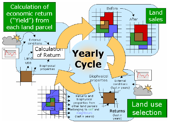
| Figure 3. The Yearly cycle in FEARLUS. Starting at the bottom right, Land Managers choose Land Uses for their Land Parcels, the Economic Return is then calculated (top left), then Land Parcel exchanged (top right) |
Land Use Selection
Calculation of Return
Land Sales
Adaptation
Fitness
Prediction
Interaction
Sensing
Stochasticity
Collectives
Observation
Land Use Choice Outcome Submodel
|
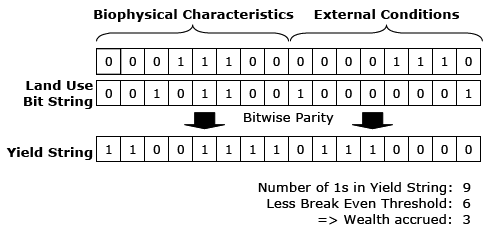
| Figure 4. Illustration of bitstring-based model of Land Use choice outcome. |
Land Use Selection
Calculation of Return
Land Sales
|
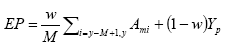
(7) |
Still, …, differences in the style of the presentation are likely to remain. We have to accept this at the current stage, because the protocol has to compromise between being general enough to include all kinds of individual- or agent-based models and being specific enough to fulfil its purpose.
|
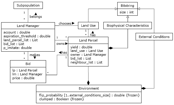
| Figure 5. UML class diagram depicting part of the structure of FEARLUS+ELMM. (Copyright 2008 IGI Global. Reprint by permission of the publisher.) |
2 For those unfamiliar with this distinction, procedural programming languages consist of a series of statements that (loops, conditionals and function or method calls aside) are executed in the order written. Declarative programming languages consist of a series of statements that could be considered to be logically axiomatic, the order of which need not matter (though this depends on the particular language being used). The program is then run by asking a question of an inference engine, which attempts to derive an answer to the question by executing an appropriate selection of the statements in an order determined by the principles on which it is built.
ANTONIOU G and van Harmelen F (2004). Web Ontology Language: OWL. In Staab S and Studer R (Eds.) Handbook on Ontologies. Berlin: Springer. pp. 67-92.
AXELROD R M (1986). An evolutionary approach to norms. American Political Science Review. 80 (4), 1095-1111.
AXTELL R, Axelrod R, Epstein J, and Cohen M D (1995). Aligning simulation models: A case study and results. Computational and Mathematical Organization Theory 1 (1), 123-141.
BARRETEAU O and others (2003). Our companion modelling approach. Journal of Artificial Societies and Social Simulation 6 (2) 1. https://www.jasss.org/6/2/1.html
BAUER B, Müller J and Odell J (2001). Agent UML: A formalism for specifying multiagent interaction. In Ciancarini P and Wooldridge M (Eds.) Agent-Oriented Software Engineering: First International Workshop AOSE 2000, Limerick, Ireland, June 10, 2000. Lecture Notes in Computer Science 1957. Berlin: Springer-Verlag. pp. 91-103.
BERRY B, Kiel L, and Elliot E (2002). Adaptive agents, intelligence, and emergent human organization: Capturing complexity through agent-based modeling. Proceedings of the National Academy of Sciences 99 (Supplement 3), 7178-88.
BIGBEE A, Cioffi-Revilla C and Luke S (2005). Replication of Sugarscape using MASON. In Troitzsch K G (Ed.) Representing Social Reality: Pre-proceedings of the Third Conference of the European Social Simulation Association, Koblenz, September 5-9, 2005. Koblenz: Verlag Dietmar Fölbach. pp. 6-15.
BOERO R and Squazzoni F (2005). Does empirical embeddedness matter? Methodological issues on agent-based models for analytical social science. Journal of Artificial Societies and Social Simulation 8 (4) 6. https://www.jasss.org/8/4/6.html
BROWN D G, Page S E, Riolo R and Rand W (2004). Agent based and analytical modeling to evaluate the effectiveness of greenbelts. Environmental Modelling and Software 19, 1097-1109.
BROWN D G, Page S E, Riolo R, Zellner M and Rand W (2005). Path dependence and the validation of agent-based spatial models of land use. International Journal of Geographic Information Systems 19, 153-174.
BROWND G and Robinson D T (2006). Effects of heterogeneity in preferences on an agent-based model of urban sprawl. Ecology and Society 11 (1): 46, http://www.ecologyandsociety.org/vol11/iss1/art46/.
CHRISTLEY S, Xiang X and Madey G (2004). Ontology for agent-based modeling and simulation. In Macal C M, Sallach D and North M J (Eds.) Proceedings of the Agent 2004 Conference on Social Dynamics: Interaction, Reflexivity and Emergence, co-sponsored by Argonne National Laboratory and the University of Chicago, October 7-9. http://www.agent2005.anl.gov/Agent2004.pdf.
CIOFFI-REVILLA C and Gotts N (2003). Comparative analysis of agent-based simulations: Geosim and FEARLUS models. Journal of Artificial Societies and Social Simulation 6 (4) 10. https://www.jasss.org/6/4/10.html.
DAVIES B, Koo B, Hunsberger C, Rothman D, Polhill G, Blackstock K, Izquierdo L, Gotts N, Ferrier R and Dunn S (2006). Story and simulation approaches to appraise possible programmes of measures for a sub basin in Scotland. Third Harmoni-CA Forum and Conference, 5-7 April 2006, Osnabrück, Germany. http://www.harmoni-ca.info/Conferences/Past_Meetings/3rd_Harmoni-CA_Forum_and_Conference/abstract%20Blackstock.pdf.
DREYFUS-LEON M and Kleiber P (2001). A spatial individual behaviour-based model approach of the yellowfin tuna fishery in the eastern Pacific Ocean. Ecological Modelling 146 (1-3), 47-56.
EDMONDS B and Hales D (2003). Replication, replication and replication: Some hard lessons from model alignment. Journal of Artificial Societies and Social Simulation 6 (4) 11, https://www.jasss.org/6/4/11.html.
FERNANDEZ L, Brown D G, Marans R and Nassauer J (2005). Characterizing location preferences in an exurban population: Implications for agent based modeling. Environment and Planning B, 32 (6), 799-820.
GALAN J M and Izquierdo L R (2005). Appearances can be deceiving: Lessons learned re-implementing Axelrod's 'Evolutionary Approach to Norms'. Journal of Artificial Societies and Social Simulation 8 (3) 2, https://www.jasss.org/8/3/2.html.
GILBERT N and Troitzsch K G (2005). Simulation for the social scientist. Open University Press.
GOSS-CUSTARD J D, Burton N H K, Clark N A, Ferns P N, McGrorty S, Reading C J, Rehfisch M M, Stillman R A, Townend I, West A D and Worrall D H (2006). Test of a behavior-based individual-based model: response of shorebird mortality to habitat loss. Ecological Applications, 16, 2215-2222.
GOTTS N M, Polhill J G and Law A N R (2003). Aspiration levels in a land use simulation. Cybernetics and Systems 34, 663-683.
GRIMM V (2007). Ecological models: Individual-based models. In Jørgensen S-E (Ed.) Encyclopedia of Ecology. Elsevier (in press).
GRIMM V, Berger U, Bastiansen F, Eliassen S, Ginot V, Giske J, Goss-Custard J, Grand T, Heinz S K, Huse G, Huth A, Jepsen J U, Jørgensen C, Mooij W M, Müller B, Pe'er G, Piou C, Railsback S F, Robbins A M, Robbins M M, Rossmanith E, Rüger N, Strand E, Souissi S, Stillman R A, Vabø R, Visser U and DeAngelis D L (2006). A standard protocol for describing individual-based and agent-based models. Ecological Modelling 198 (1-2), 115-126.
GRIMM V and Railsback S F (2005). Individual-based Modeling and Ecology. Princeton University Press, Princeton, NJ.
GRIMM V, Revilla E, Berger U, Jeltsch F, Mooij W M, Railsback S F, Thulke H-H, Weiner J, Wiegand T and DeAngelis D L (2005). Pattern-oriented modeling of agent-based complex systems: lessons from ecology. Science 310, 987-991.
HARE M and Deadman P J (2004). Further towards a taxonomy of agent based simulation models in environmental management. Mathematics and Computers in Simulation 64 (1), 25-40.
HARPER, S J, Westervelt J D and Trame A-M (2002). Management application of an agent-based model: control of cowbirds at the landscape scale. In Gimblett H R (Ed.) Integrating Geographic Information Systems and Agent-Based Modeling Techniques for Understanding Social and Ecological Processes. Oxford University Press.
KALDOR N (1961/1968). Capital Accumulation and Economic Growth. In Lutz, F A and Hague, D C (Ed.): The Theory of Capital. Reprint. London: Macmillan, pp. 177-222.
KOO B K, Dunn S M and Ferrier R C (2004). A spatially-distributed conceptual model for reactive transport of phosphorus from diffuse sources: an object-orientated approach. In Pahl-Wostl C, Schmidt S and Jakeman T (Eds.) IEMSs 2004 International Congress: Complexity and Integrated Resources Management, International Environmental Modelling and Software Society, Osnabrück, Germany, 14-17 June 2004.
MARANS R W (2003). Understanding environmental quality through quality of life studies: The 2001 DAS and its use of subjective and objective indicators. Landscape and Urban Planning 65 (1-2), 75-85.
MATHEVET R, Bousquet F, Le Page C and Antona M (2003). Agent-based simulations of interactions between duck population, farming decisions and leasing of hunting rights in the Camargue (Southern France). Ecological Modelling 165: 107-126.
MOSS S, Gaylard H, Wallis S and Edmonds B (1998). SDML: A multi-agent language for organizational modelling. Computational & Mathematical Organization Theory 4 (1), 43-69.
PARKER D C (1999). Landscape outcomes in a model of edge-effect externalities: A computational economics approach. SFI Publication 99-07-051. Santa Fe, NM: Santa Fe Institute. http://www.santafe.edu/research/publications/workingpapers/99-07-051.pdf.
PARKER D C (2005). Agent-based modelling to explore linkages between preferences for open space, fragmentation at the urban-rural fringe, and economic welfare. Paper presented at The Role of Open Space and Green Amenities in the Residential Move from Cities, December 14-16 2005, Dijon, France.
PARKER D C, Berger T and Manson S M (2002). Agent-Based Models of Land-Use and Land Cover Change: Report and review of an international workshop, October 4-7, 2001, Irvine, California, USA. LUCC Report Series No. 6. Anthropological Center for Training and Research on Global Environment Change, Indiana University, USA: LUCC Focus 1 Office.
PARKER D C, Brown D G, Polhill J G, Deadman P J and Manson S M (2008). Illustrating a new 'conceptual design pattern' for agent-based models and land use via five case studies: The MR POTATOHEAD framework. In Lopez Paredes A and Hernandez Iglesias C (Eds.) Agent-Based Modelling in Natural Resource Management Valladolid, Spain: Universidad de Valladolid, pp. 23-51.
PARKER D C and Meretsky V (2004). Measuring pattern outcomes in an agent-based model of edge-effect externalities using spatial metrics. Agriculture, Ecosystems and Environment 101, 233-250.
PIOU P, Berger U, Hildenbrandt H, Grimm V, Diele K and D'Lima C (2007). Simulating cryptic movements of a mangrove crab: recovery phenomena after small scale fishery. Ecological Modelling 205, 110-122.
PITT W C, Box P W and Knowlton F F (2003). An individual-based model of canid populations: modelling territoriality and social structure. Ecological Modelling, 166, 109-121.
POLHILL J G, Gotts N M and Law A N R (2001). Imitative versus nonimitative strategies in a land use simulation. Cybernetics and Systems 32 (1-2), 285-307.
POLHILL J G, Parker D C and Gotts N M (2005). Introducing land markets to and agent based models of land use change. In Troitzsch K G (Ed.) Representing Social Reality: Pre-proceedings of the Third Conference of the European Social Simulation Association, Koblenz, September 5-9, 2005. Koblenz: Verlag Dietmar Fölbach. pp.150-157.
POLHILL J G, Parker D C and Gotts N M (2008). Effects of land markets on competition between innovators and imitators in land use: results from FEARLUS-ELMM. In: Hernandez, C., Troitzsch, K. and Edmonds, B. (Eds.), Social Simulation Technologies: Advances and New Discoveries. New York: IGI Global. pp. 81-97.
POLHILL J G, Pignotti E, Gotts N M, Edwards P and Preece A (2007). A semantic grid service for experimentation with an agent-based model of land use change. Journal of Artificial Societies and Social Simulation 10 (2) 2, https://www.jasss.org/10/2/2.html.
RAILSBACK S F (2001). Concepts from complex adaptive systems as a framework for individual-based modelling. Ecological Modelling, 139, 47-62.
RAILSBACK S F and Harvey, B C (2002). Analysis of habitat selection rules using an individual-based model. Ecology, 83, 1817-1830.
RAND W, Brown D G, Page S E, Riolo R, Fernandez L E and Zellner M (2003). Statistical validation of spatial patterns in agent-based models. Proceedings of Agent Based Simulation 4, Montpellier, France, 2003.
RICHIARDI M, R Leombruni R, Saam N and Sonnessa M (2006). A Common Protocol for Agent-Based Social Simulation. Journal of Artificial Societies and Social Simulation 9 (1) 15. https://www.jasss.org/9/1/15.html.
RIOLO R L, Cohen M D and Axelrod R (2001). Evolution of cooperation without reciprocity. Nature 411, 441-443.
SCHWEIK C, Evans T and Grove J M (2005). Open source and open content: A framework for global collaboration in social-ecological research. Ecology and Society 10 (1): 33. http://www.ecologyandsociety.org/vol10/iss1/art33/.
WANG M and Grimm V (2007). Home range dynamics and population regulation: an individual-based model of the common shrew. Ecological Modelling 205, 397-409.
WILENSKY U (1999). Netlogo. http://ccl.northwestern.edu/netlogo/. Center for Connected Learning and Computer-Based Modeling, Northwestern University, Evanston, IL.
WILENSKY U and RAND W (2007) Making models match: replicating an agent-based model. Journal of Artificial Societies and Social Simulation 10 (4) 2. https://www.jasss.org/10/4/2.html
ZELLNER M L, Riolo R, Rand W, Page S E, Brown D G and Fernandez L E (2003). The interaction between zoning regulations and residential preferences as a driver of urban form. 2003 UTEP Distinguished Faculty and Student Symposium, Urban and Regional Planning Program, University of Michigan. April, 2003.
 Return to Contents of this issue
© Copyright Journal of Artificial Societies and Social Simulation, [2008]