Abstract

The Schelling model of segregation is an agent-based model that illustrates how individual tendencies regarding neighbors can lead to segregation. The model is especially useful for the study of residential segregation of ethnic groups where agents represent householders who relocate in the city. In the model, each agent belongs to one of two groups and aims to reside within a neighborhood where the fraction of 'friends' is sufficiently high: above a predefined tolerance threshold value F. It is known that depending on F, for groups of equal size, Schelling's residential pattern converges to either complete integration (a random-like pattern) or segregation. The study of high-resolution ethnic residential patterns of Israeli cities reveals that reality is more complicated than this simple integration-segregation dichotomy: some neighborhoods are ethnically homogeneous while others are populated by both groups in varying ratios. In this study, we explore whether the Schelling model can reproduce such patterns. We investigate the model's dynamics in terms of dependence on group-specific tolerance thresholds and on the ratio of the size of the two groups. We reveal new type of model pattern in which a portion of one group segregates while another portion remains integrated with the second group. We compare the characteristics of these new patterns to the pattern of real cities and discuss the differences.

Keywords:

Schelling Model, Ethnic Segregation, Minority-Majority Relations

Introduction

1.1

The Schelling model of segregation (Schelling 1971, 1978) is one of the earliest agent-based models of social science. The model was introduced by Thomas Schelling to illustrate how individual incentives and individual perceptions of difference can lead collectively to segregation (Schelling 1978 p. 148). While the model is indicative of a variety of phenomena where individuals tend to relocate according to the share of similar neighbors, it was found especially useful for the study of residential segregation.

The original model

1.2

In the Schelling model, agents occupy cells of rectangular space. A cell can be occupied by a single agent only. Agents belong to one of two groups and are able to relocate according to the fraction of friends (i.e., agents of their own group) within a neighborhood around their location. The model's basic assumption is as follows: an agent, located in the center of a neighborhood where the fraction of friends f is less than a predefined tolerance threshold F (i.e., f < F), will try to relocate to a neighborhood for which the fraction of friends is at least f (i.e., f ≥ F) (Schelling 1978 p. 148). Note that a high threshold value of F corresponds to a low agent's tolerance to the presence of strangers within the neighborhood.

1.3

Schelling studied the dynamics generated by this simple relocation rule for the case of two groups of equal size and a common tolerance threshold F for both groups. The study revealed the existence of a critical tolerance threshold F_segr ≈ 1/3 such as, for F < F_sgr initially random pattern remains, in time, random-like, while for F ≥ F_sgr initially random pattern converges to a segregate pattern (Figure 1).

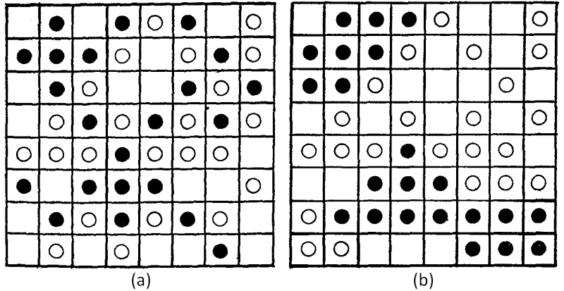
Figure 1. (a) initial condition of one of Schelling's experiments; (b) stable segregated pattern obtained in several iterations (Schelling 1974)

1.4

Two results of Schelling's study are regarded as central: (a) the value of F_sgr is essentially lower than the intuitively expected value of 1/2; (b) the change of the limit pattern from pseudo-random to segregated as F passed the value of F_sgr is abrupt, thus the model does not produce intermediate patterns.

Schelling model versus real-world residential patterns

1.5

Real-world residential dynamics is mainly governed by economic factors and, thus, Schelling model patterns are usually considered as having greater theoretical than applied importance. However, in some cases direct correspondence between the model patterns and real residential distributions can be established. Our study is motivated by one of these cases: the Jewish-Arab ethnic residential distribution in Israeli cities. Based on the Israeli population census of 1995 (Benenson and Omer 2003), we were able to construct patterns for ethnically mixed Israeli cities at the resolution of individual houses, which is equivalent to the resolution of the Schelling model.

1.6

Empirical evidence supports Schelling-like views of the residential interactions between the Jewish and Arabs families in Israel; both tend to reside in neighborhoods that have sufficient numbers of residents of their ethnic group (Omer 1996). Thus, we can consider residential patterns in the mixed Israeli cities as a "stylized" outcome of the residential choice of Schelling's residential agents.

1.7

We consider the residential pattern of Arab Muslims, Arab Christians and Jews in the cities of Yaffo and Ramle, both of which are located in central Israel. Yaffo is actually the southern part of the city of Tel Aviv-Yaffo while Ramle is located 15 km south-east of Yaffo. The ethnic pattern of Yaffo in 1995 is presented in Figure 2. The city contains segregated Arab and Jewish areas; in Ajami, a neighborhood in the center (Area A), Christians and Muslims live together, and in Yaffo-Daled, a neighborhood in the south (Area B), the population is Jewish. Some of the boundaries between Jewish and Arab areas in Yaffo are sharp (Area D), while some are extended (Area C).

1.8

The ethnic residential pattern of the city of Ramle is presented in Figure 3 and is more complex than Yaffo. Large areas of the city are populated almost solely by Jews (Area A), while some are populated almost exclusively by Muslims (Area B). The city contains integrated areas (Area C), which, unlike Yaffo, are remote from the segregated Arab areas. The city also contains areas populated by Muslims and Christians (Area D) and an area where Christians and Jews coexist (Area E).

1.9

Yaffo and Ramle patterns are thus essentially more variable than the integrated and segregated patterns characteristic of the Schelling model: the pattern contains homogeneous patches of Arab and Jewish populations and several integrated areas with different fractions of Arab and Jewish populations in each. Yaffo's integrated patches are at the boundary between the segregate patches; in Ramle segregated and aggregated areas are not necessarily adjacent and can be separated by the non-populated areas.

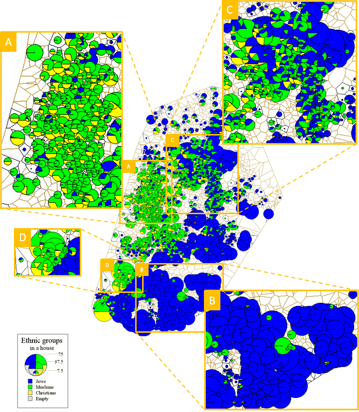
Figure 2. Ethnic residential distribution of Yaffo in 1995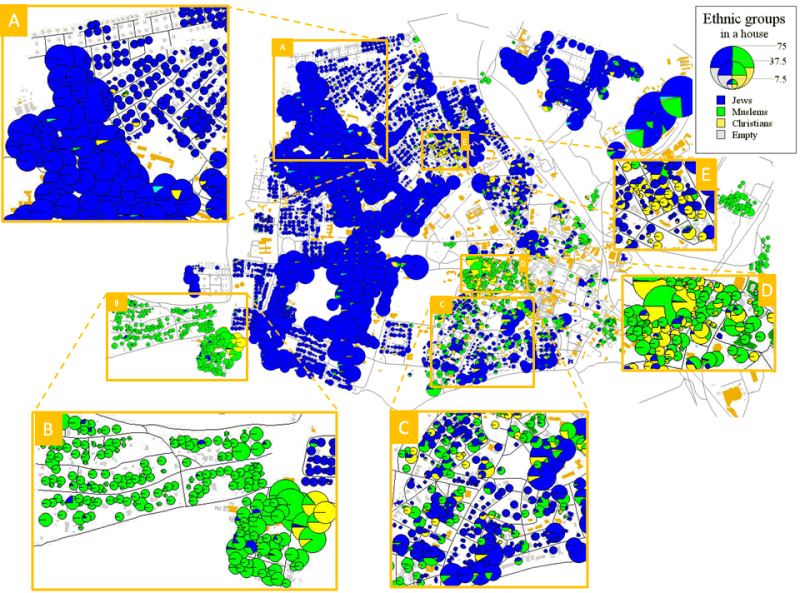

Figure 3. Ethnic residential distribution of Ramle in 1995

1.10

Several explanations for this qualitative difference between the observed patterns and Schelling's theoretical patterns can be proposed. First, ignoring economics, Yaffo and Ramle patterns are still in a developmental stage, thus some of the patterns may be temporary. Second, low-income Jews and Arabs may not be able to avoid living together, while the richer Jews and Arabs are able to segregate. Third, contrary to the previous explanation, poor Jews and Arabs may be intolerant of each other and thus segregate, while wealthy householders may be tolerant and thus stay together. Each of these explanations could be tested if the data on migration activity and individual wealth were available. However, taking Yaffo and Ramle patterns as a source of inspiration, can the observed patterns still be explained within the non-economic Schelling framework?

1.11

To simplify let us consider the Muslim and Christian Arabs as a single group. Conceptually, in the Jewish-Arab residential patterns of Yaffo and Ramle, we can specify three qualitatively different configurations (Figure 4):

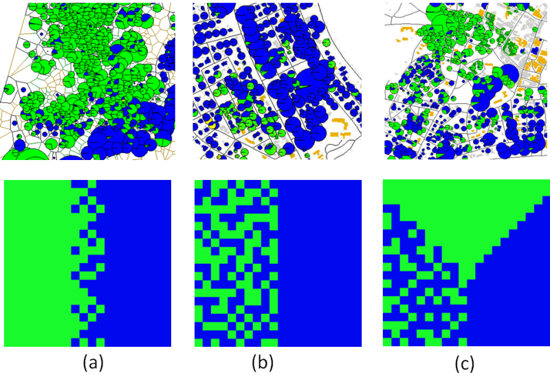
Figure 4. Three qualitatively different patterns in Yaffo and Ramle and the corresponding Schelling-like patterns: (a) two segregated patches; (b) segregated patch adjacent to integrated patch; (c) integrated patches adjacent to two segregated patches

1.12

In the first pattern (Figure 4a), two segregated groups are separated by a narrow boundary of transition. In the second pattern (Figure 4b), the majority of members of one of the groups are segregated while some of the members are integrated with the members of the other group. The third and most complex pattern (Figure 4c) presents two segregated groups, each adjacent to the integrated area.

1.13

In this paper, we demonstrate that the variety of Schelling model patterns is greater than the random-segregated dichotomy and that the patterns in Figures 4a and 4b, can be generated by the model if the numbers of two groups or group tolerance thresholds are different. However, the Schelling model does not generate persistent patterns that contain segregated patches of both groups together with integrated patches, as in Figure 4c.

1.14

The structure of the paper is as follows: Section 2 presents the state-of-the-art of Schelling model studies and describes the kind of dynamics that generates the patterns that are neither segregated nor integrated (we call them mixed). Section 3 formally describes the model and the methodology of the study. The results of the study are presented in Section 4 and are followed by the discussion in Section 5.

Schelling model studies

Irregular partition of space

2.1

Studies of the Schelling model focus on conditions enabling segregation and on the characteristics of the patterns produced by the model. As can be expected, the model results are qualitatively robust to the structure of residential space. Irregular partition of the plane into polygonal units and neighborhood definition based on polygon adjacency do not change the main results of the pattern's dichotomy and the abrupt transition from integrated to segregated limit pattern (Flache and Hegselmann 2001). Laurie and Jaggi (2002, 2003) supplemented this finding by systematically investigating Schelling model dynamics as depending on the size of the neighborhoods and revealed, as should be expected, that the size of homogeneous patches increases with the growth of the neighborhood radius while the number of homogeneous patches in patterns decreases.

Asymmetric relations, more than two groups

2.2

Portugali et al. (1994, 1995) showed that Schelling model patterns converge toward segregation even if only agents of one group react to the fraction of friends while agents of the other group are indifferent. However, in that case the tolerance threshold that separates systems converging toward integrated as opposed to segregated patterns is essentially higher than the value of 1/3, characteristic for the symmetric case. Benenson (1998) investigated the Schelling model for the case of several groups of agents characterized by several binary characteristics. In addition to integrated and segregated stable patterns, he revealed unstable but persistent regimes in which homogeneous patterns of the agents of one or more groups are repeatedly self-organizing and vanishing.

Accounting for economic differences between agents

2.3

Several studies (Benard and Willer 2007; Benenson 1999; Fossett 2006b; Portugali 2000; Benenson and Hatna 2009) consider agents characterized by continuous "economic status," which can be compared with the cells' price. The agents search for neighborhoods that are both "friendly" and "sufficiently wealthy." As might be expected, system dynamics become more variable in this case, depending on how the agents' residential preferences depend on the neighbors' group identity and status.

Agents that exchange places

2.4

A qualitatively different way of modeling agents' relocation is to assume that unsatisfied agents exchange their places rather than search for a vacancy over all unoccupied cells. This view attracted the attention of several researchers (Pollicott and Weiss 2001; Zhang 2004), who also assume that the preferences of agents are non-monotonous, and they might prefer neighborhoods with a low fraction of foreigners to those occupied exclusively by friends. The dynamics of the model patterns in this case are also more complex than the integrated-segregated dichotomy. However, the mathematical properties of these models differ qualitatively from the standard settings and we thus consider this formulation as different from Schelling's original model.

The "Bounded Neighborhood" model

2.5

Another variant of the Schelling model is the "Bounded Neighborhood" model that was also presented by Schelling (1978, p. 155) but is less popular than the version discussed above. In the "Bounded Neighborhood" version, instead of a regular grid, the grid is divided into blocks, which are essentially larger than the neighborhoods of the popular version of the model. No matter where the agent is located within the block, it reacts to the fraction of friends all over it, and leaves the block if the fraction of friends is below the tolerance threshold F. Different agents, however, can react to different threshold fractions of friends within the block, and the main parameter of the "Bounded Neighborhood" model is the distribution of the agents' F-values.

2.6

The analytic investigation of this version of the model was started by Schelling (1978) and continued by Clark (1991, 1993, 2002, 2006). They have demonstrated that both groups can persist in a block in case agents of each type essentially vary in their tolerance to strangers. However, the equilibrium is not globally stable and, depending on initial conditions, block's population can converge to a segregated or aggregated state for the same distributions of tolerance.

2.7

A spatial version of the "Bounded Neighborhood" model, in which the agents' population consists of more than two ethnic groups and residential agents react to the population structure and migrate among adjacent blocks in case of unsatisfied demands, has been investigated in depth in a series of recent simulations by Fossett (Fossett and Waren 2005; Fossett 2006a; Fossett 2006b), who also directly relates the model's results to residential patterns in the real-world cities. Fossett aimed at reflecting the situation in the United States and considered three residential groups—White, Black and Hispanic—who also differ in their economic status. The aggregate units used are 7 × 7 cell blocks and the city is represented by the 12 × 12 grid of blocks. Fossett (2006a) investigated the relationship between ethnic and status segregation and concluded that this interaction might limit our ability to integrate the ethnic groups. Specifically, he pointed out that reduction in housing discrimination by race may not necessarily lead to large declines in ethnic segregation.

Application of the Schelling model for real cities

2.8

Several attempts to apply the Schelling model to the real-world situation (Benenson et al. 2002; Koehler and Skvoretz 2002; Bruch and Mare 2006) provide likelihood approximations of the segregated or more complex residential distributions observed in cities. In what follows we limit ourselves to abstract models and do not delve into greater details of these implementations.

"Liquid" and "Solid" dynamics

2.9

A general insight into the relation between the rules and the patterns engendered by the Schelling model was suggested by Vinkovic and Kirman (2006), who consider a continuous analog of the Schelling model. Namely, they start with representing eight cells of the 3 × 3 neighborhood as eight equal sectors, and then weaken the discrete representation of space by considering each sector's angle as a continuous variable. The continuous representation makes it possible to describe the model dynamics by means of differential equations and to further investigate the dynamics of the boundaries of the homogeneous clusters.

2.10

The analysis of the continuous model results in a differentiation between two fundamental types of relocation rules for the Schelling model: rules that specify Schelling's system as representing solid-like matter and rules that specify it as representing liquid-like matter (Vinkovic and Kirman 2006). The Schelling model represents "solid matter" if the rules enable relocation to a better location only. In this case, the system stalls when converging to a pattern in which none of the agents can improve their state. Usually, the solid Schelling pattern stalls after about ten time steps, with an essential fraction of agents who are dissatisfied with their location but unable to find a better one. The rules that allow relocation to cells of the same utility result in liquid-like dynamics. The liquid Schelling system does not stall even if all the agents are satisfied with their location and, eventually, reaches a persistent state where the characteristics of the pattern (such as level of segregation) do not change, vast majority of agents are satisfied with their location and rare migrations result in slow and non-directed evolution of patch boundaries.

2.11

Vinkovic and Kirman (2006) demonstrate that the persistent patterns of the model that allows relocation to better locations only are numerous and depend on the details of the model rules, while the persistent patterns of the "liquid" view of relocation are just two: integrated and segregated. They also claim that the model dynamics are robust to variations in the rules' details insofar as the set of rules result in "solid" or "liquid" pattern dynamics.

2.12

The solid-liquid dichotomy is relatively new and the studies of the Schelling model we are aware of do not specify explicitly whether the model rules permit agents to relocate between cells of the same utility. However, when applying Schelling's view to the real world, it seems necessary to enable relocation between residences of the same utility in order to reflect numerous reasons of household migrations that are not captured by the neighborhood and ethnic based view, say, distance to facilities or jobs.

2.13

Following Vinkovic and Kirman's (2006) view, we investigated a set of rules that on the one hand directly interprets Schelling's idea of resident's reaction to the fraction of friends in the neighborhood as a determinant of the residential choice, and on the other hand enables migration between cells of the same utility, i.e., entails a liquid-like dynamics (Benenson and Hatna 2011). The study of the model reveals qualitatively new results: the variety of its patterns is greater than random-segregated dichotomy. Namely, for a sufficiently wide range of parameters, the model pattern converges to a mixed state, in which an essential portion of one group segregates while the rest of its members remain integrated with the other group.

The mixed patterns

2.14

The mixed patterns are qualitatively different from the well-known segregated and integrated ones. To illustrate, let us consider a city with a 0.2:0.8 ratio of group sizes. In this case, for values of F within the interval of ˜ (0.08, 0.17), an initially random pattern converges, in time, to a state in which part of the area is occupied by the majority exclusively, while the rest of the area is aggregated (Figure 5). As we have demonstrated numerically and supported analytically (Benenson and Hatna 2009; Benenson and Hatna 2011), the values of F that generate mixed patterns are lower than F_sgr.

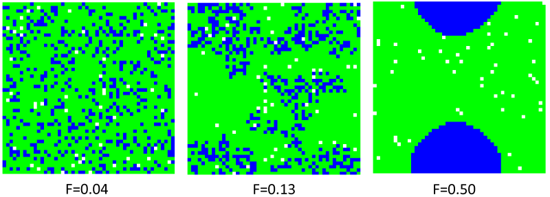
Figure 5. (a) integrated (b) mixed and (c) segregated persistent patterns produced by the Schelling model for the 0.2:0.8 Blue-to-Green size ratio

2.15

Mixed patterns further undermine the view of the Schelling model as robust to variations of assumptions. The qualitatively different patterns obtained for the unequal group numbers manifest the possibility that the emergence of real-world residential patterns, as those presented in Figures 2-4, can still be qualitatively explained by the Schelling model. The deviation from the 1:1 ratio of the groups' sizes is only one of several possible alterations of the "commonly accepted" settings. These settings, however, are just a tradition and are not related to the basic Schelling assumption of agents who aim at residing within friendly neighborhoods. There are several other unnecessary settings, such as the assumptions of equal tolerance threshold of members of both groups, identical reaction of agents of a given group to neighbors and agents' identical view of the neighborhood size and form.

2.16

In this paper, we investigate two alterations of the standard assumptions: we study Schelling model dynamics in the case of non-equal groups and non-equal tolerance thresholds of the groups (which are still identical for all agents within the group). We demonstrate that the mixed patterns are typical for a population of highly but not absolutely tolerant agents and discuss the extent to which this formal result can explain the real-world residential patterns as observed in Yaffo and Ramle.

Formalization of the model and the methodology of investigation

3.1

In this paper, we apply the model rules defined in Benenson and Hatna (2011).

Formal representation of the model rules

3.2

Let us denote an agent as a, a cell as h and the neighborhood of h, excluding h itself, as U(h). We consider U(h) to be a Moore's square n × n neighborhood (Moore 1970) and denote the fraction of a's "friends" (i.e., agents belonging to a's group) among all agents located within the neighborhood U(h) as f_a(h). Note that we ignore empty cells within U(h).

3.3

City space: N × N grid of cells on a torus, the latter used to avoid boundary effects. A cell cannot be occupied by more than a single agent. There is no emigration or immigration.

3.4

There are two groups of residential agents: Blue (B) and Green (G).

3.5

Time: discrete time, asynchronous updating (Cornforth et al. 2005). We follow Schelling's view of residential behavior and assume that agents observe the system's changes immediately after they occur. At each time step, every agent decides whether and where to relocate. Agents are considered in random order, which is established anew at each time step.

3.6

Agent's a tolerance threshold F_a: following Schelling's view, we assume that an agent a located at h is satisfied if the fraction of friends within U(h) is F_a or higher. As the tolerance threshold is common for all agents of the Blue or Green group, we denote it as F_B or F_G respectively.

3.7

Neighborhood's U(h) utility for a: we define the utility u_a(h) of the neighborhood U(h) for a as:

ua(h) = min(fa(h), Fa)/Fa if Fa > 0

(1)

and assume that u_a(h) = 1 if F_a = 0 (absolutely tolerant agent a) (Figure 6)

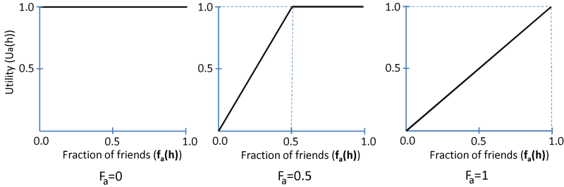
Figure 6. The utility of location h for an agent a as a function of the fraction of friends, fa, within U(h): (a) absolutely tolerant agent (Fa = 0), (b) agent seeking for 50% of friends (Fa = 0.5), (c) absolutely intolerant agent (Fa = 1)

3.8

Agent's residential behavior: at each time step t, an agent a located at h decides whether to relocate or remains at h. When relocating, an agent a considers w vacant locations and compares their utility to the utility of its current location h. The awareness of a about vacancies does not depend on the vacancies' distance to h.

3.9

Agent a performs its relocation decision in two steps:

Step 1: Decides whether to relocate:
- Generates a random number p, uniformly distributed on (0, 1).
- If (u_a(h) < 1 or (u_a(h) = 1 and p < m)) then tries to relocate, otherwise stays at h.

Step 2: If the decision is "to relocate," then searches for a new location and decides whether to move there:
- Memorizes the utility u_a(h) of the current location h.
- Constructs a set V(a) of relocation opportunities by randomly selecting w vacancies from all cells that are vacant at that moment.
- Estimates utility u_a(v) of each v ∈ V(a) for a, and selects one of the highest utility u_a(v_best). If there are several best vacancies in V(a), chooses one of them randomly.
- Moves to v_best if either
u_a(h) < 1 and u_a(v_best) > u_a(h), the utility of v_best is higher than that of h, or
u_a(h) = 1 and u_a(v_best) = 1 , the utility of h is high and the move to v_best is unrelated to the number of friends in the neighborhood,
- Otherwise stays at h.

For m > 0, the above model rules entail liquid-like dynamics. Note, however, that only agents who are satisfied with their location are allowed to relocate to a vacancy of equal utility; unsatisfied agents can move to higher utility vacancies only.

3.10

It is important to emphasize the manner in which agents choose vacancies. According to the definition of a neighborhood's utility (Equation 1), agents are satisficers (Simon 1982) who regard a location h as satisfactory as long as the fraction of friends f_a within U(h) is equal or higher than their tolerance threshold F_a. All satisfactory locations are of the same utility 1, and agents do not distinguish between them.

The methodology of model investigation

3.11

We investigate the persistent model patterns based on a 50 × 50 torus, assuming that 2% of the cells are empty (d =2%). We assume that the rate of spontaneous relocation attempts is 1% per iteration (m = 0.01) and an agent considers at most 30 vacancies when trying to relocate (w = 30).

3.12

In discrete cell space, the number of cells in the neighborhood excluding the central cell determines the series of possible tolerance thresholds F. For fully occupied 3 × 3 Moore neighborhood of eight cells, this series would be F = 0/8, 1/8, … 7/8, 8/8. Schelling (1971) employed a 3 × 3 Moore neighborhood. However, nine possible values of F are insufficient for understanding the model dynamics. We thus use a 5 × 5 Moore neighborhood, which results in the series of 25 F-values (0/24, 1/24, …, 24/24), sufficient for representing the model phenomena in full.

3.13

In what follows, we investigate model patterns as depending on the:

• Fraction β of Blue agents.
• Tolerance threshold F_B of Blue agents.
• Tolerance threshold F_G of Green agents.

3.15

We assume that the Blue agents are minority and investigate model patterns for the series of β-values: 0.05, 0.15, …, 0.5. As explained above, the series of values for F_B and F_G are 0/24, 1/24, …, 24/24.

3.16

Figure 7 presents the 3D "half-cube" of the investigated parameters' space. We begin the study of model patterns with the parameter's values on the cube's surface and then combine the results in order to describe model patterns for all values of β, F_B and F_G.

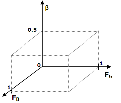
Figure 7. Parameter space of the Schelling model as investigated in this paper

3.17

To ensure that the model patterns are not dependent on initial conditions, all model runs are repeated starting with two initial patterns: random and fully segregated (Figure 8).

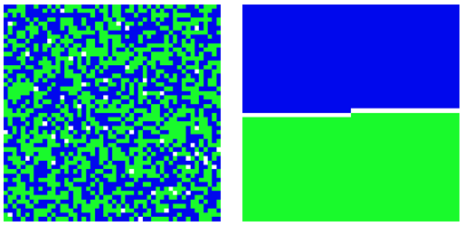
Figure 8. Model initial patterns (a) random, (b) fully segregated

Characterization of model patterns

The use of Moran's I for recognizing integrated and segregated patterns

3.18

In what follows we characterize the global properties of the Blue and Green agents' patterns using the Moran's index I of spatial association (Anselin 1995; Getis and Ord 1992; Zhang and Linb 2007) applied to binary data (Lee 2001; Griffith 2010).

3.19

The Moran's I statistic is calculated for the spatial variable x_h over the occupied cells according to (2). The variable x_h is defined as follows: x_h = 0 if h is occupied by Blue agent and x_h = 1 if h is occupied by Green agent.

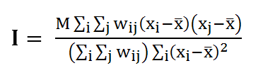
(2)

where x_i, x_j denote the values of x_h in cells i, j; M = Round((1-d)×N²) is the overall number of occupied cells, x bar is the mean value of x_h over the occupied cells, w_ij = 1 if j ∈ U(i), and w_ij = 0, otherwise.

3.20

A value of Moran's I close to 0 represents a random (integrated) pattern while a value close to 1 represents complete segregation (see Zhang and Linb 2007 for a review). Based on the permutation test for the 50 × 50 torus city, critical values of Moran's I equals 0.002 at p = 0.01. In what follows, we consider a city pattern as random if Moran's I is below 0.002. We run simulations for 50,000 time steps, which are sufficient for the pattern to reach a persistent state, if exist, or exhibit fluctuations (see below). The characteristics of the patterns were calculated for 10,000 time interval between the iteration 40,000 and 50, 000.

Three possible parts of the mixed pattern

3.21

The Moran's I calculated over the entire city area is useful for distinguishing between fully integrated (random) patterns, for which Moran's I is close to zero, segregated patterns, for which I is close to 1 and other (mixed) patterns, for which Moran's I is higher than 0 but lower than 1. However, the value of Moran's I cannot distinguish between the two types of mixed patterns presented in Figures 4b and 4c; for both of these the value of Moran's I would be intermediate. To distinguish between these types of patterns, we employ the following algorithm that recognizes the two segregated and the "residual" parts of the city as presented in Figures 4a-c (the size of all the neighborhoods below are 5 × 5):

1. Identify the segregated (Blue and Green) parts:
   Loop by all occupied cells and identify the Blue cells that have only Blue neighbors and the Green cells that have only Green neighbors. Denote these two cell sets as B^ and G^ respectively.
2. Identify the boundary of the segregated parts:
   Loop by all occupied cells that do not belong to B^ or G^, and identify the cells which neighborhoods have non-empty overlap with G^ or B^. Denote this set of cells as E1^.
3. Identify the boundary of the residual part of the city and combine it with the boundary of the segregated parts:
   Loop by all occupied cells that do not belong to B^, G^ or E1^, and identify those, neighborhoods which have non-empty overlap with E1^. Denote these cells as E2^ and unite E1^ and E2^ into E^.
4. Denote the cells that do not belong to B^, G^ or E^ as M^.
   

Figure 9 presents the algorithm steps for the patterns in Figures 4b and 4c. As stated above, the model city is a torus.

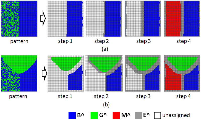
Figure 9. The algorithm for identifying segregated (B^, G^), boundary (E^) and residual (M^) parts, applied to the pattern (b) and (c) in Figure 4b

3.22

Below we distinguish between the patterns in Figures 4b and 4c based on the size of the segregated Blue c(B^), segregated Green c(G^) and residual c(M^) parts in the city. Namely, we define the C-index as:

C = min(c(B^), c(G^), c(M^))/N2

(3)

The real-world and abstract patterns in Figure 4 contain either two or all three possible parts, and the relative area of each part is high. We thus classify a pattern as of the Figure 4c type if the value of C is at least 10% (C ≥ 10%). High C-value threshold of 10% guarantees that each of the three parts could be visually recognized in the pattern, as characteristic of the real-world patterns in Figure 4.

Persistent and fluctuating patterns

3.23

Our setting of the Schelling model allows for spontaneous relocation and, thus, the model residential pattern never stalls. However, for the majority of β, F_B and F_G values the pattern converges to persistent state, in which its segregation characteristics do not change significantly. When it is clear from the context, we use "model pattern" when referring to "model persistent pattern."

3.24

For some combinations of parameters the patterns do not stabilize. An extreme example is the case of F_G = 3/24, F_B = 7/24, β = 0.5. As can be seen from Figure 10a, the Moran's I for this set of parameters fluctuates, in time, between 0.35 - 0.70 and so does the C-index, which fluctuates between 0 and 15%. Figure 10b presents two extreme patterns generated for this set of parameters: one segregated, qualitatively similar to the pattern presented in Figure 4a, and the other mixed, qualitatively similar to the pattern presented in Figure 4c. The left pattern is characterized by the relatively high value of Moran's I and low value of the C-index while the right pattern is characterized by the relatively low value of Moran's I and high value of the C-index.

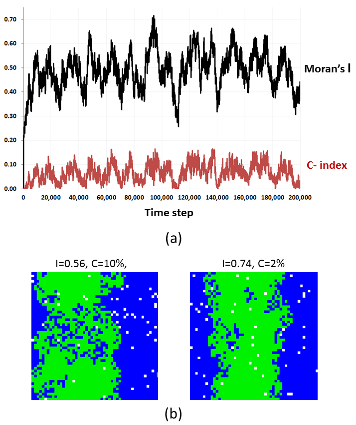
Figure 10. The fluctuating pattern of FG = 3/24, FB =7/24,β=0.5: (a) The dynamics of Moran's I and C-index for the first 200,000 iterations (b) Typical mixed and segregated patterns observed.

Results of the model investigation

4.1

In what follows, we briefly repeat the classic model results (§4.2) and proceed with investigating the model behavior as dependent on all three parameters β, F_B and F_G. §4.6-§4.11 deal with special subsets of the (β, F_B and F_G) parameter space. §4.18 onwards considers the general situation.

Basic case: equal groups of equal tolerance thresholds (β = 0.5, F_G = F_B = F)

4.2

To verify Schelling's conclusions regarding the case of groups of equal size and tolerance thresholds (Figure 11), we performed 25 model runs for which F_G = F_B = F = 0/24, 1/24, …, 24/24, and, in addition, nine runs with F_G = F_B = F = 0/8, 1/8, …, 8/8 that aimed to investigate the influence of the neighborhood size on model patterns.

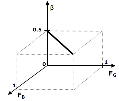
Figure 11. The investigated set of parameters β = 0.5, FG = FB

4.3

The Moran's I values as dependent on F are presented in Figure 12.

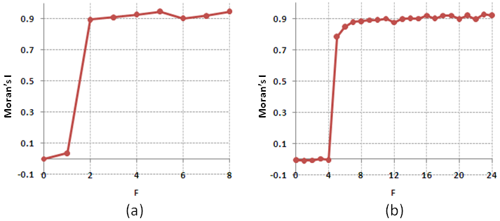
Figure 12. Moran's I for model persistent patterns as dependent on F for (a) 3 × 3 (b) 5 × 5 neighborhoods

4.4

Qualitatively, our results are fully consistent with Schelling's findings. Namely, the interval of the F-values consists of two subsets: F ≤ 4/24 and F ≥ 5/24. For F ≤ 4/24, the patterns are random (integrated), while for F ≥ 5/24 the patterns are segregated. The transition between the two subsets is abrupt. In the case of the 3×3 neighborhood, the results are qualitatively the same but less precise: random patterns are characteristic of F ≤ 1/8 = 3/24, while for F ≥ 2/8 = 6/24 the patterns are segregated.

4.5

The patterns for the case of the 5×5 neighborhood are presented in Figure 13. The unsmooth boundary of the segregated pattern of F = 5/24 seems to correspond to the conceptual pattern of Figure 4a. For the segregated patterns (F ≥ 5/24), the higher F, the smoother the boundary between the clusters of agents of the same color. This explains the slow growth of Moran's I with the growth of F in Figure 12.

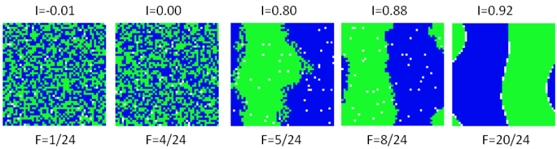
Figure 13. Persistent model patterns for the case of equal groups as depending on F

Persistent patterns for the 2D-subsets of parameters

4.6

In what follows, we investigate the model persistent patterns for the case of Green majority versus Blue minority and values of parameters limited to three 2D subspaces of the 3D half-cube (Figure 14):

• β ∈ (0, 0.5], F_B = F_G: equal tolerance of both groups (Figure 14a);
• β ∈(0, 0.5], F_G = 0, F_B ∈ [0, 1]: absolutely tolerant Green majority (Figure 14b);
• β ∈(0, 0.5], F_G ∈ [0, 1], F_B = 0: absolutely tolerant Blue minority (Figure 14c).

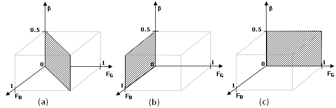
Figure 14. Three investigated 2D-subsets of parameters (a) β ∈(0, 0.5], FB = FG, (b) β ∈(0, 0.5], FG = 0, FB ∈ [0, 1], (c) β ∈(0, 0.5], FG ∈ [0, 1], FB = 0

4.7

Following Benenson and Hatna (2011), we denote, for a given β, F_rnd,β as the highest value of F that generates random (integrated) persistent pattern (characterized by close to zero value of the Moran's I) and F_sgr,β as the lowest value of F that entails a segregated pattern (characterized by close to unit value of the Moran's I). As shown above, for β = 0.5, the values of F_rnd,0.5 and F_sgr,0.5 are adjacent, i.e., F_rnd,0.5 = 4/24, and F_srg,0.5 = 5/24.

Blue minority versus Green majority, equal tolerance threshold in both groups (β ∈ (0, 0.5], F_B = F_G = F)

4.8

As presented in §2.14, the case of unequal groups exhibits mixed patterns. To illustrate, let us consider the case of β = 0.2. The values of Moran's I for the persistent pattern as dependent on F = F_B = F_G and the patterns for selected values of F are presented in Figure 15.

4.9

As can be seen in Figure 15a, the dependence of the model pattern on F in case of β = 0.2 is different than for the case of β = 0.5. Namely, for F = 2/24, 3/24 and 4/24 the values of Moran's I are non-zero, but yet lower than that characteristic of the segregated patterns. As can be observed in Figure 15b, the patterns for these three values of F are neither random nor segregated. According to Figure 15, F_rnd,0.2 = 1/24, while F_sgr,0.2 = 5/24 (note that the values of F_sgr,0.2 and F_sgr,0.5 are the same, and equal to 5/24). For the values of F ∈ (F_rnd,0.2, F_sgr,0.2), part of the city area is occupied by the Green majority exclusively while the rest of the area is integrated. As it is shown in Benenson and Hatna (2009, 2011), with the growth of F, the integrated part of the integrated region becomes more compact, thus entailing a growth of the Moran's I. The city abruptly segregates when F increases from 4/24 to 5/24. For F ≥ 5/24, the Moran's I value slowly increases with an increase in F and the boundary between the Green and Blue clusters becomes smoother, just as for β = 0.5.

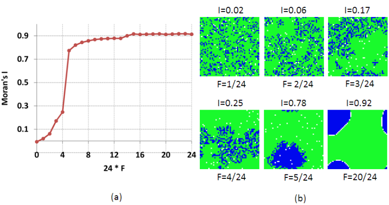
Figure 15. (a) Moran's I and (b) persistent patterns as dependent on F, for β = 0.2

4.10

The complete view of Moran's I dependence on F and β is presented in Figure 16a. Note that (a) for β > 0.05 the pattern abruptly segregates when F passes the threshold value of F_sgr,β = 5/25, while for β = 0.05, F_sgr,0.05 = 6/25; (b) the value of F_rnd,β decreases linearly and the width of the interval of the F-values generating the mixed patterns increases with the decrease in β. The dependence of the C-index on F and β is presented in Figure 16b. It indicates that for all F ≠ 5/24 the patterns consist of two parts only, either of segregated Blue and Green or of segregated Green and mixed parts. For F= 5/25, the maximal values of C are positive but far below the 10% level we accepted as characteristic of the complex pattern in Figure 4c. The non-zero C-index obtained for F = 5/24 characterizes essential non-smoothness of the boundary between the segregated Blue and Green areas. The type of pattern as dependent on β, F_B, F_G, is shown in Figure 16c. In a theoretical study (Benenson and Hatna 2009) we have demonstrated that for F ∈ (F_rnd,β, F_sgr,β), in case of the mixed pattern, the distribution of the Green and Blue agents within the integrated part is random. It is important to note that the fraction of minority within these patches is always higher than β, grows with the growth of β and reaches 0.5 when F approaches F_sgr,β. The latter explains the abrupt change from mixed to segregated pattern when F passes the threshold value of F_sgr,β .

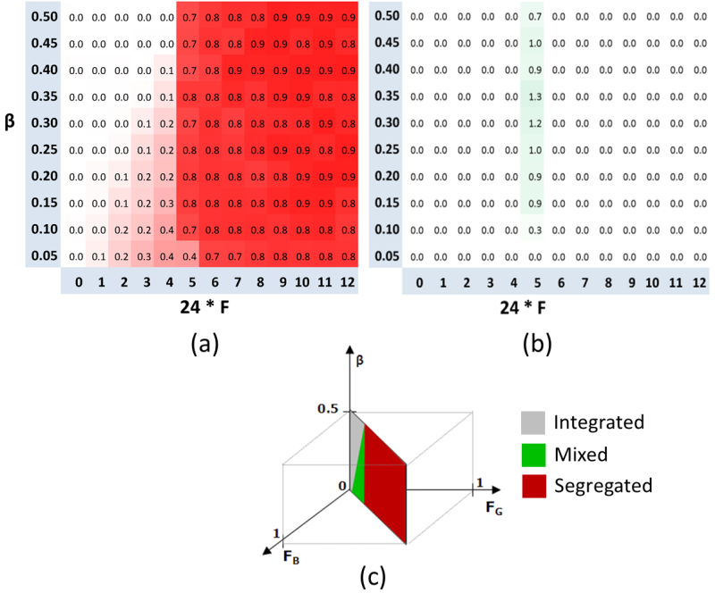
Figure 16. The dependence of (a) Moran's I and (b) C-index on F for β = 0.05, 0.15, …, 0.5 and FB = FG = F and (c) the sets of parameters characteristic of the random, mixed and segregated patterns in the half cube

Absolutely tolerant group (β ∈ (0, 0.5], F_G = 0 or F_B =0)

4.11

In this section, we examine the case in which agents of one groups are completely tolerant. We start by describing the case of equal size groups (β = 0.5) and completely tolerant Green agents (F_G = 0) and then describe the case where the tolerant group is either a majority or minority.

4.12

The case of equal groups (β = 0.5) and completely tolerant agents of one of the groups is briefly mentioned by Portugali et al. (1997), who noted that despite the absolute neutrality of members of one group, the residential pattern segregates when the tolerance threshold of the other group is sufficiently high. Our simulations essentially extend this result. As above, for given β, we denote as F_B,rnd,β the highest value of F_B that entails a random pattern and as F_B,sgr,β the lowest value of F_B that entails a segregated pattern.

4.13

Figure 17 presents the dependence of Moran's I on F_B for the case of β = 0.5 and F_G = 0 and the patterns for selected values of F. According to Figure 17a F_B,rnd,0.5 = 4/24 and Moran's I, value increases linearly with further increase of F_B until F_B reaches F_B,sgr,0.5 = 13/24. Unlike the case of F_G = F_B, there is no abrupt change in the level of segregation when F_B approaches F_B,sgr,0.5. For F_B ∈ [5/24, 12/24] the pattern is mixed.

4.14

The corresponding persistent patterns are shown in Figure 17b. Part of the area of the mixed patterns is occupied exclusively by the fully tolerant Green agents, while few Green agents reside within the integrated part of the patterns. The Blue agents avoid neighborhoods where their fraction is below F_B, and, thus the fraction of fully tolerant Greens residing within the Blue-dominated areas decreases with the increase in F_B. For F_B = 10/24, 11/24 and 12/23, the patterns slightly fluctuate in time, because of the few Green agents that reside within the Blue area. However, the C-index always remains below 3%.

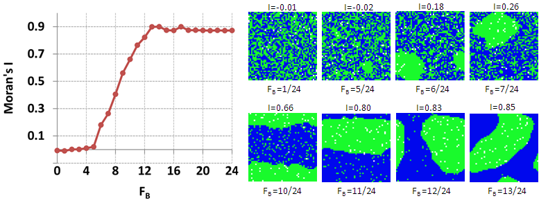
Figure 17. Characteristics of model persistent pattern for FG = 0, β = 0.5: (a) Moran's I as dependent on FB; (b) persistent patterns for selected values of FB

4.15

The dependences of Moran's I and C on β and F_B for the case of absolutely tolerant majority or minority are presented in Figure 18. For a tolerant majority (Figure 18c), a decrease in β entails a decrease in F_B,rnd,β and F_B,sgr,β, but at different rates and with the length of the (F_B,rnd,β, F_B,sgr,β) interval thus increasing. The dependence of Moran's I on F_G and β for the case of absolutely tolerant Blue minority is presented in Figure 18a. In this case, the decrease in β results in the growth of both F_G,rnd,β and F_G,sgr,β and a reduction of the interval of mixed patterns to zero when β decreases to 0.15. The three domains of parameters for both cases are presented in Figure 18e. The C-index (Figure 18b, 18d) is non-zero for the values of F just below the threshold that guarantees full segregation, namely F_B, F_G = 10/24 11/24 and 12/23. The model patterns for these values of F slightly fluctuate in time.

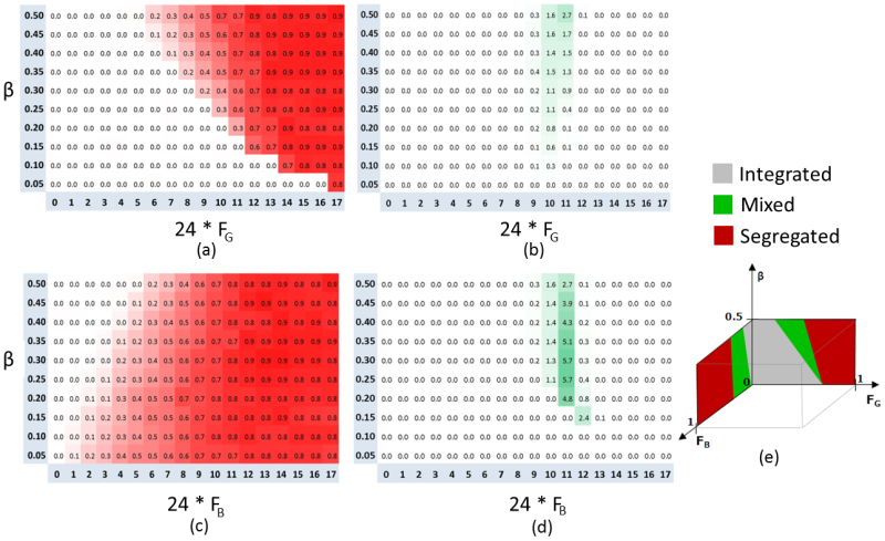
Figure 18. Moran's I in case of absolutely tolerant majority or absolutely tolerant minority: (a) absolutely tolerant Blue minority (FB = 0); (b) absolutely tolerant Green majority (FG = 0); (c) parameters characteristic of the random, mixed and segregated patterns

4.16

Persistent patterns for the case of absolutely tolerant Green majority and β = 0.3 are presented in Figure 19a (F_B,rnd,0.2 = 3/24, F_B,sgr,0.2 = 13/24). Just as for β = 0.5, with the growth of F_B within (F_B,rnd,0.2, F_B,sgr,0.2), the fraction of absolutely tolerant Green agents residing within the Blue-dominated areas decreases with the growth of F, until, at F_B = 13/24, complete segregation is reached. Figure 19b presents the series of persistent patterns for the case of absolutely tolerant Blue minority β = 0.3. Just as in the case of absolutely tolerant majority, the fraction of minority within the majority-dominated area decreases with an increase in F_G, and, in parallel, the size of the minority patches increases.

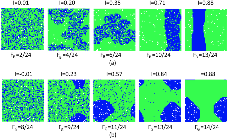
Figure 19. Model's persistent patents for β = 0.3: (a) completely tolerant Green majority (FG = 0); (b) completely tolerant Blue minority (FB = 0)

4.17

Overall, the persistent patterns in case of absolutely tolerant minority do not differ from those obtained for the case of absolutely tolerant majority. The interval of the F-values, for which these patterns are produced, becomes narrower and shifts toward the higher values of F with the decrease in β.

General case

4.18

To complete the description of the model persistent patterns, let us consider their dependence on all three parameters: β, F_B and F_G. We do that for four horizontal cross-sections of the half-cube at β = 0.05, 0.2, 0.35, and 0.5. The four surfaces of Moran's I and C for F_G ≤ 17/24 and F_B ≤ 17/24 and corresponding 3D illustration of the full (F_B, F_G, β) domains producing random, mixed and segregated patterns are presented in Figure 20.

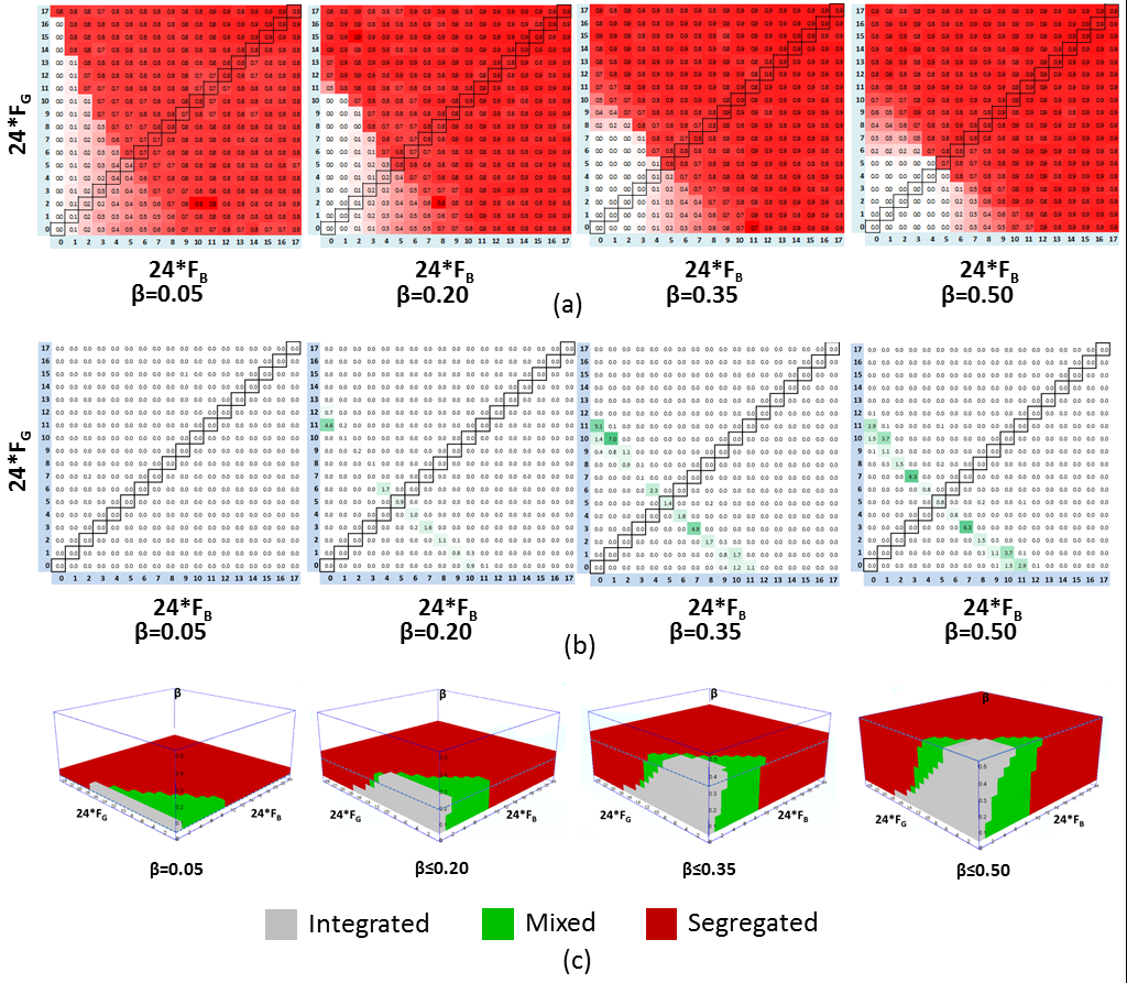
Figure 20. (a) Moran's I and (b) C-index as dependent on (FG, FB) for FG ≤ 17/24, FB ≤ 17/24 (for larger FG or FB the patterns are always segregated) and β = 0.05, 0.2, 0.35 and 0.5 (the cases of FB = FG are marked); (c) the 3D presentation of the (FB, FG, β) domains producing random, mixed, and segregated patterns

4.19

With the increase in β, the domain of (F_B, F_G) values producing mixed patterns in the left-top increases. This domain represents the case of a tolerant minority group which become more numerous as β increases and thus contributes more to the emergence of mixed patterns. Correspondingly, with the increase in β the domain of (F_B, F_G) values producing mixed patterns in the right-button decreases as the number of tolerant majority agents decreases. The (F_B, F_G) domain becomes symmetric across the F_B = F_G when β reaches 0.5. The domain of the (F_B, F_G) values producing the integrated patterns is largest for β = 0.5 and shrinks with the decrease in β; the mixed pattern area grows at its expense.

4.20

All the persistent patterns produced in the (β, F_B, F_G) domain are characterized by zero or very low value of the C-index (figure 20b). The non-zero values of C are obtained for values of parameters that lie on the boundary of the domain that guarantees segregation, namely, for the values of F_B and F_G that satisfy the condition F_B + F_G = 10/24, 11/24, 12/24. For these values of F_B and F_G, the patterns fluctuate in time, and the amplitude of the fluctuations of the Moran's I and C-index does not depend on β. For few (F_B, F_G) pairs on this boundary, the amplitude of the fluctuations reaches the level of F_G = 3/24, F_B = 7/24, β = 0.5 (Figure 10). We defer investigation of this phenomena to future work.

Discussion

5.1

Our version of the Schelling model is based on two qualitative assumptions: first, agents are satisficers, i.e., they do not distinguish between locations where the number of friends is above their tolerance threshold; second, the relocation rules allow satisfied agents to migrate between vacancies of the same utility. The satisficing principle is consistent with Schelling's original formulation (Schelling 1978), while the relocation rules entail liquid-like dynamics that prevent patterns from stalling in a state where some of the agents are dissatisfied because no satisfactory vacancies are available.

5.2

We demonstrated that satisficers, who can relocate between neighborhoods of the same utility, remain randomly distributed in space if their demands for having friends within neighborhoods is low, segregate if their demands are high and produce mixed patterns when their demands for friends within the neighborhood are intermediate. In the latter case, the population pattern depends on the investigated parameters: the fraction of minority β and the level of tolerance F_B and F_G of the agents of each group.

5.3

Can we relate these results to the real-world patterns as observed in Ramle and Yaffo (Figures 2-4)? Basically, yes: Arab householders are minorities in Yaffo and Ramle and empirical evidence suggests that members of Arab minorities living in mixed cities in Israel are somewhat indifferent to the presence of Jewish neighbors in their building or in neighboring buildings (Benenson et al. 2002). We can also assume that Israeli Arabs and Jews are satisficers in regard to the ethnic structure of their residential neighborhoods and probably use additional criteria, besides ethnicity of neighbors, when searching for a dwelling. Our research demonstrates that if these tendencies characterize the entire population groups, the residential dynamics entail mixed patterns that are indeed observed over parts of Yaffo and Ramle.

5.4

The model generated persistent patterns that are consistent with two of the three patterns presented in Figure 4: segregated patterns such as the one presented in Figure 4a, and mixed patterns such as the one in Figure 4b. However, Yaffo and Ramle patterns are more complex than those obtained in the model scenarios investigated in this paper: they both contain mixed parts side by side with segregated ones, as is schematically represented in Figure 4c. As we have shown above, the Schelling model even in extended, three-dimensional, parameter space does not produce such persistent patterns. Stated formally, within the model framework that we investigated in this paper, no matter what the fraction of minority or tolerance thresholds of the two groups, segregated and mixed areas cannot permanently coexist.

5.5

The patterns in which segregated and mixed areas coexist emerge and dissolve periodically for values of F that lie on the boundary between the domains of parameters that entail persistently segregated and persistent mixed patterns. These fluctuating patterns should be further investigated in order to assess their robustness to the variation in the model rules, especially if we further generalize the model and assume that the level of tolerance among Green and Blue agents can vary.

5.6

A preliminary investigation demonstrates that more complex patterns than those obtained in this paper can indeed be obtained in this case, and these patterns contain one integrated and two segregated regions for a range of parameters that is wider than that revealed in this paper. We believe that such a generalization takes the model closer to the reality. Indeed, the assumption that members of an ethnic group are identical in their attitude to members of another ethnic group seems artificial no matter which groups are under discussion. However, the only result in this respect regarding Arabs and Jews is the ongoing empirical study by Omer et al. (2012), who demonstrate that Jews and Arabs in Yaffo essentially vary in their residential tolerance to the members of the other group.

Acknowledgements

The authors would like to thank the editor and two anonymous reviewers for their helpful comments.

References

ANSELIN, L. (1995) Local Indicators of Spatial Association - LISA. Geographical Analysis 27(2): 93-115. [doi:10.1111/j.1538-4632.1995.tb00338.x]

BENARD, S. and Willer, R. (2007) A Wealth and Status-Based Model of Residential Segregation. The Journal of Mathematical Sociology 31(2): 149-174. [doi:10.1080/00222500601188486]

BENENSON, I. (1998) Multi-agent simulations of residential dynamics in the city. Computers, Environment and Urban Systems 22: 25-42. [doi:10.1016/S0198-9715(98)00017-9]

BENENSON, I. (1999) Modeling population dynamics in the city: from a regional to a multi-agent approach. Discrete Dynamics in Nature and Society 3(2-3): 149-170. [doi:10.1155/S1026022699000187]

BENENSON, I. and Omer, I. (2003) High-resolution Census data: a simple way to make them useful. Data Science Journal (Spatial Data Usability Special Section) 2(26): 117-127. [doi:10.2481/dsj.2.117]

BENENSON, I., Omer, I., Hatna, E. (2002) Entity-based modeling of urban residential dynamics - the case of Yaffo, Tel-Aviv. Environment and Planning B. 29: 491-512. [doi:10.1068/b1287]

BENENSON, I. and Hatna E. (2009) The Third State of the Schelling Model of Residential Dynamics. arXiv:0910.2414v1 [physics.soc-ph].

BENENSON, I. and Hatna, E. (2011) Minority-Majority Relations in the Schelling Model of Residential Dynamics. Geographical Analysis. 43:287-305. [doi:10.1111/j.1538-4632.2011.00820.x]

BRUCH, E. E. and Mare, R. D. (2006) Neighborhood Choice and Neighborhood Change. American Journal of Sociology 112(3): 667-709. [doi:10.1086/507856]

CLARK, W. A. V. (1991) Residential Preferences and Neighborhood Racial Segregation: A Test of the Schelling Segregation Model. Demography 28(1): 1-18. [doi:10.2307/2061333]

CLARK, W. A. V. (1993) Search and choice in urban housing markets. Behavior and Environment: Psychological and Geographical Approaches. T. Gärling and R. G. Golledge. Amsterdam, Elsevier/North Holland: 298-316.

CLARK, W. A. V. (2002) Ethnic preferences and ethnic perceptions in multi-ethnic settings. Urban Geography 23: 237-256. [doi:10.2747/0272-3638.23.3.237]

CLARK, W. A. V. (2006) Ethnic Preferences and Residential Segregation: A Commentary on Outcomes from Agent-Based Modeling. The Journal of Mathematical Sociology 30(3): 319 - 326. [doi:10.1080/00222500500544128]

CORNFORTH, D., Green D. G. and Newth, D.. (2005) Ordered asynchronous processes in multi-agent systems. Physica D 204: 70-82. [doi:10.1016/j.physd.2005.04.005]

FLACHE, A. and Hegselmann, R. (2001) Do Irregular Grids make a Difference? Relaxing the Spatial Regularity Assumption in Cellular Models of Social Dynamics. Journal of Artificial Societies and Social Simulation vol. 4, no. 4 4(4) 6: http://www.soc.surrey.ac.uk/JASSS/4/4/6.html.

FOSSETT, M. A. (2006a) Ethnic Preferences, Social Distance Dynamics, and Residential Segregation: Theoretical Explorations Using Simulation Analysis. Mathematical Sociology 30(3-4): 185 - 273. [doi:10.1080/00222500500544052]

FOSSETT, M. A. (2006b) Including preference and social distance dynamics in multi-factor theories of segregation. Mathematical Sociology 30(3-4): 289-298. [doi:10.1080/00222500500544151]

FOSSETT, M. A. and Waren, W. (2005) Overlooked Implications of Ethnic Preferences for Residential Segregation in Agent-based Models. Urban Studies 42(11): 1893-1917. [doi:10.1080/00420980500280354]

GETIS, A., and Ord, J. (1992) The analysis of spatial association by use of distance statistics. Geographical Analysis 24:189-206. [doi:10.1111/j.1538-4632.1992.tb00261.x]

GRIFFITH, D. (2010) The Moran Coefficient for Non-Normal Data. Journal of Statistical Planning and Inference 140, 2980-2990. [doi:10.1016/j.jspi.2010.03.045]

KOEHLER, G. and Skvoretz, J. (2002) Preferences and Residential Segregation: A Case Study of University Housing. http://web1.cas.usf.edu/MAIN/include/0-1201-000/casestudy.pdf. Accessed September 13th, 2010.

LAURIE, A. J. and Jaggi, N. K. (2002) Physics and Sociology: Neighbourhood Racial Segregation. Solid State Physics (India) 45: 183-184.

LAURIE, A. and Jaggi, J. N. K. (2003) Role of Vision in Neighbourhood Racial Segregation: A Variant of the Schelling Segregation Model. Urban Studies 40(13): 2687-2704. [doi:10.1080/0042098032000146849]

LEE, S-I (2001) Developing a bivariate spatial association measure: an integration of Pearson's r and Moran's I. Journal of Geographical Systems 3: 369-385. [doi:10.1007/s101090100064]

MOORE, E. F. (1970) Machine models of self-reproduction. In A. W. Burks, ed, Essays on Cellular Automata, pages 187-203. Univ of Illinois Press.

OMER, I. (1996) Ethnic Residential Segregation as a Structuration Process. Unpublished Ph.D Thesis, Tel-Aviv University, Tel-Aviv.

OMER I. Romann M. and Goldblatt R. (2012) Tolerance and Geographic Scale in the Urban Area. Submitted to the Journal of Urban Affairs.

POLLICOTT, M. and Weiss, H. (2001) The Dynamics of Schelling-Type Segregation Models and a Nonlinear Graph Laplacian Variational Problem. Advances in Applied Mathematics 27: 17-40. [doi:10.1006/aama.2001.0722]

PORTUGALI, J. (2000) Self-Organization and the City. Berlin, Springer. [doi:10.1007/978-3-662-04099-7]

PORTUGALI, J. and Benenson, I. (1995) Artificial planning experience by means of a heuristic sell-space model: simulating international migration in the urban process. Environment and Planning B 27: 1647-1665. [doi:10.1068/a271647]

PORTUGALI, J., Benenson I. and Omer, I. (1994) Socio-spatial residential dynamics: stability and instability within a self-organized city. Geographical Analysis 26(4): 321-340. [doi:10.1111/j.1538-4632.1994.tb00329.x]

PORTUGALI, J., I. Benenson, Omer, I. (1997) Spatial cognitive dissonance and sociospatial emergence in a self-organizing city. Environment and Planning B-Planning & Design 24(2): 263-285. [doi:10.1068/b240263]

SCHELLING, T. C. (1971). Dynamic models of segregation. Journal of Mathematical Sociology 1: 143-186. [doi:10.1080/0022250X.1971.9989794]

SCHELLING, T .C. (1974) On the ecology of micromotives. The Corporate society. Marris, R. (ed). London: Macmillan: 19-64.

SCHELLING, T. C. (1978) Micromotives and Macrobehavior. New York, WW Norton.

SIMON, H. A. (1982) Models of bounded rationality. Cambridge, MIT Press.

VINKOVIC, D. and KIRMAN, A. (2006) A physical analogue of the Schelling model. PNAS 103(51): 19261-19265. [doi:10.1073/pnas.0609371103]

ZHANG, J. (2004) Residential segregation in an all-integrationist world. Journal of Economic Behavior & Organization 54: 533-550. [doi:10.1016/j.jebo.2003.03.005]

ZHANG, T. and Linb, G. (2007) A decomposition of Moran's I for clustering detection. Computational Statistics & Data Analysis 51: 6123-6137. [doi:10.1016/j.csda.2006.12.032]