Abstract

Slums provide shelter for nearly one third of the world's urban population, most of them in the developing world. Slumulation represents an agent-based model which explores questions such as i) how slums come into existence, expand or disappear ii) where and when they emerge in a city and iii) which processes may improve housing conditions for urban poor. The model has three types of agents that influence emergence or sustenance of slums in a city: households, developers and politicians, each of them playing distinct roles. We model a multi-scale spatial environment in a stylized form that has housing units at the micro-scale and electoral wards consisting of multiple housing units at the macro-scale. Slums emerge as a result of human-environment interaction processes and inter-scale feedbacks within our model.

Keywords:

Slums, Housing, Developing Countries, Urban Poor, Informal Settlements, Agent-Based Modeling

Introduction

1.1

Over 900 million people live in either slums or squatter settlements, a number projected to increase to approximately 2 billion by 2030 (UN-Habitat 2003). Most of this growth is expected in the developing world especially in Asia and Africa. It is predicted that many large cities in developing countries will nearly double their population by 2020, but the development of formal housing will not be able to keep pace with this rapid urbanization (UN-Habitat 2003). The estimates given above for slum population are based on the definition suggested by UN-Habitat (2006), one of the most widely used definitions of slums. According to this definition, a household is a slum dweller if it lacks any of the following five elements: i) access to water, ii) access to sanitation, iii) secured tenure, iv) durable housing, and v) sufficient living area. An advantage of this definition is that it defines a slum at the household level. Most other definitions define a slum at the neighborhood level (e.g. Census of India 2001; Neuwirth 2005; Roy and Alsayyad 2004), thereby making it difficult to differentiate between living conditions of the households within a slum.

1.2

The problems of inadequately serviced and overcrowded housing usually occupied by economically weaker sections of society are not new. Historical accounts of slums in Europe and the Americas between the 17th and 19th century suggest possibly worse slum conditions than that seen in the developing world today. Few cities can grow without the expansion of slums and informal employment in their initial growth period (Mumford 1961).

1.3

The international development community has recognized the proliferation of slums as an important societal issue for rapidly urbanizing developing countries. As a response, Target 11 of the Millennium Development Goals (MDG) aims to significantly improve lives of 100 million slum dwellers by 2020 (United Nations 2000). National and Local governments in many developing countries have also called for slum up-gradation and slum improvement programs. For example, the current president of India recently announced a policy targeted to make India slum-free within the next five years (Times of India 2009), which has resulted in a massive housing programme in India (MHUPA 2010). The expansion of urban renewal programs and a greater focus on making cities slum-free has taken a front seat among policymakers in most developing countries around the world.

1.4

While a variety of policy actions, ranging from forced evictions to participatory slum improvements, have been taken to improve the lives of slum dwellers, slum-free cities still remain a distant goal for most developing countries. For the policies to be more effective, it is essential to understand how slums come into existence, how they expand, and finally which processes improve housing conditions for the urban poor. This paper attempts to explore these kinds of questions using a simulation approach. The paper is organized as follows: we briefly review past efforts of slum modeling before describing our agent-based model named Slumulation. We then verify our model and present simulation results from Slumulation. Finally, we conclude the paper with discussion and remarks on areas of further work.

Previous Efforts to Model Slums

2.1

Slum formation has been a subject of interest for several disciplines: urban geography, economics, sociology, politics, environmental science and demography to name but a few. There have been several attempts to explain the forces behind slum formation. Here we only present a brief review of the prominent residential location and slum formation models, which are the most closely related to the model presented below. The Burgess (1927) model (part of the "Chicago School") was the first model in urban geography to identify where "working men's housing" and "zones in transition" were located in the form of ghettos and slums in inner city locations. Over time the "Chicago School" became more rigorous with the advances in neo-classical economics. In particular, the works of Alonso (1964), Muth (1969) and Mills (1972) which demonstrated how a "rent-gradient" of declining prices and rents away from the center could be calculated to predict the locations of various groups of people within a city.

2.2

There have been several attempts to explain slum formation using urban census data with models largely known as factorial ecology (see Janson 1980 for a review). Amongst them is Shevky and Bell's (1955) model of social area analysis which showed that households were spatially separated from each other based on five key factors: i) socio-economic status, ii) familism, iii) ethnicity, iv) accessibility/space trade-off and v) socio-economic disadvantage. While such work allows one to define different areas of a city, the approach has often been criticized for lacking a link between theories of social change and the realities of areal differentiation within cities (Johnston 1971). For example, these works tell us little about the behavior and reasoning of why people decide to move to a specific type of area.

2.3

The majority of previous models that explored slum formation and city growth approached the problem as a static phenomenon (e.g.Alonso 1964), which has been challenged with the growing realization that urbanization and slum formation are largely dynamic processes. Dynamic models that accommodate this flux and complexity are thus called for (Batty 2005). Agent-based modeling (ABM) provides an ideal framework to study such dynamic processes because they focus on individual agent's behavior and their interactions give rise to a global phenomena of interest. For example, in Schelling's (1971) model of segregation, individuals are given the simple rule of choosing a location based on only one-third of neighbors of similar race. But this rule, when applied to many individuals, gives rise to a highly segregated spatial pattern globally. Secondly, cities are complex systems, which are more than a simple sum of their parts (Batty 2005). A simulation approach provides us an opportunity to explore the possibility of sub-systems (e.g. slums) being complex themselves but also being a part of an overall complex system (e.g. the city).

2.4

While there is a growing amount of work focusing on agent-based models and urbanization (see, for instance, Benenson and Torrens 2004; Batty 2005; Heppenstall et al. 2011), the use of agent-based models for exploring slum formation is still in its infancy. Only a handful of attempts have been made to explain slum formations using ABM, principal amongst them are Sietchiping (2004); Barros (2005); Vincent (2009) and Augustijn-Beckers et al. (2011). Sietchiping (2004)'s cellular-automata (CA) model is one of the earliest simulation-based attempts to predict informal settlements as a type of land-use by adapting the CA-based urban growth model called SLEUTH (originally developed by Clarke et al. (1997) to incorporate informal settlements. However, such a model does not capture individual behavior and focuses more on mathematical cell transitions from previous states of the system. One of the first attempts to develop an agent-based model incorporating household behavior particularly focusing on slums is that of Barros (2005). The model explored how decentralized decision-making can be incorporated into slum modeling. Augustijn-Beckers et al. (2011) advanced ABM in the slum literature by creating an agent-based model based on empirically founded behavioral rules. Furthermore, Vincent (2009) demonstrated that socio-economic characteristics of the inhabitants of a city plays a significant role in shaping growth pattern of informal settlements.

2.5

While all these efforts took different approaches to model informal settlements, four main points emerge. The first is that explicit modeling of the spatial environment is important as slums emerge in distinct areas. Secondly, slums are a result of human-environment interactions. Thirdly, individual households make locational choices and lastly, local government plays an important role as it takes city-wide actions such as slum eviction or slum up-gradation to alter the slum conditions or to eradicate them. The models discussed above incorporate one or some of these aspects but none of them incorporates all of them into a single modeling framework.

2.6

Our study attempts to model a city system where several slums form, grow and disappear as a result of human-environment interactions at multiple spatial scales. For example, the household level behavior is confronted with the city level political forces in a multi-scale environment. This point of view calls for creating a human-environment interaction model where the human behavior is modeled in a multi-scalar spatial environment. Hence, our model attempts to incorporate the complexity of urban morphology combined with the social complexity of human behavior in a stylized manner. Although, multi-scale modeling of urban systems is not a completely new idea (O'Sullivan 2009), this is the first attempt to build a multi-scale model of slum formation to the best of our knowledge.

Slumulation: An Agent-based model of Slum Formation

3.1

The key idea behind Slumulation is to conduct "thought experiments" and ask "what-if" type of questions related to slum formation (Epstein and Axtell 1996). It is a stylized model a la Schelling (1971). However, Schelling's (1971) model focused on the gap between desired and available structure of the neighborhoods. Slumulation focuses on agent-environment interaction where the gap between agents' economic ability and the price and availability of dwelling units in the environment becomes of greater importance.

3.2

In terms of Axtell and Epstein (1994) schema of classification, models that portray a caricature of the agents behavior are called "Level 0" models whereas those attaining qualitative agreement with the patterns of emerging "macro-structures" are "Level 1" models. While a "Level 2" model attains quantitative agreements of emerging macro-structures, a "Level 3" model attains quantitative agreements with both emergent macro-structures as well as individual agent's micro-behavior. As shown below, the model presented here is far from Level 2 and Level 3 at this stage of development, however it is in qualitative agreement with empirical macro-structure of slum patterns in cities, and hence represents a "Level 1" type of model.

3.3

Slumulation is conceptualized as a spatial agent-based model of a city that consists of agents, their attributes, behavioral and transition rules tied to spatial entities (e.g. places to live), which all interact through space and time. We describe each of these elements in detail below, first describing the main agents before discussing their behavioral and transition rules. The classical theories and prior modeling efforts (discussed in the previous section) provide a basis for our assumptions regarding these elements of Slumulation.

3.4

The main agents that influence the slum formation process as identified from the literature are households, developers and local politicians (Parthasarthy and Pothana 1981; Singh 1986; Chege 1981; Bharucha 2011). In Slumulation, the household agents make housing location decisions; the developer agents create housing units on vacated housing sites thus adding to the existing housing stock; while the politician agents provide a subsidy to slum-dwellers in a hope to gain votes from them. This subsidy discounts the "economic rent" in varying degrees, which in turn facilitates the retention or eviction of existing slums within an area. In Slumulation, households are on the demand side while developers and politicians control the supply in the housing market, however, both developers and politicians operate at different spatial scales. Consequently, the environment is built on two spatial scales.^[1] The first layer models housing sites in which households make locational decisions on where to live and developers make development decisions. The second layer consists of electoral wards, in which politicians play their role.

Household Agents

3.5

Households are the key agents in this model. One of the most important attributes for households is their income level. Based on the income level, each household finds an affordable place to live. If rent goes beyond what a household can afford, they consider relocating to an affordable place in the next time period. As with many exploratory agent-based models (e.g. Schelling 1971), the time frame for the model is purely hypothetical but is considered as yearly intervals. Households also belong to one of the three income-groups, low, middle or high. For simplicity it is assumed that households can only share a housing site with the same income-group when they choose to live in a multi-family housing unit within a single housing site. Nonetheless, there is no restriction on living within a neighborhood of a higher income group. We assume that there is an implicit preference for living close to higher income groups as long as households can afford it. Poor households who cannot afford a housing unit could consider sharing it with other households. If they do not find another household to share within a specific time-frame, they are forced to move to an affordable place elsewhere. How long a household can sustain residing at a given location despite an unaffordable rent depends on the household's financial "staying power" i.e. households in the low-income group cannot pay unaffordable rents for a long period compared to those in the high-income group. Financial staying power is discussed further below.

Developer Agents

3.6

Developers construct housing units in order to gain profits. They buy vacant properties that were once occupied. The acquired properties are then developed, usually with a larger number of units (e.g. an apartment building at a site of a previous single family house). Developers hold a property until all the newly developed units are occupied by households. A developer agent is activated only on a housing site that is completely vacated and remains active only until all units are occupied. The developers are not explicitly shown as visual objects in the model interface but their actions are incorporated within the model processes. The developers' behavior is simple in the model presented here, but we plan to elaborate it in future versions of Slumulation. For example, the number of units to be developed varies and is chosen randomly in the current implementation but in future versions, we plan to equip them to sense the demand for housing at a particular location and build accordingly. While we have not implemented this in the current version of the model, they may also consider occupied sites for development and bid a price to buy it (and potentially compete with other developers interested in the same property). In the same spirit, they may offer kickbacks to politician agents to get a slum evicted in order to develop a brownfield site.

Politician Agents

3.7

In the model politicians monitor the demographics of their electoral wards. Each ward consists of multiple households. Politicians reduce the "effective rent" for slum-dwellers in proportion to the percent of slum population in each ward in a hope to win votes from the slum-dwellers. This relates to the notion of an implicit subsidy provided in the form of favorable policies such as protection against eviction and thus excluding a slum site from entering a formal market primarily to create an electorate (Glaeser and Shleifer 2003; Murray 2010). Slum dwellers living in wards with a higher proportion of slum households pay lower rents than those living in the wards with a lower proportion of slum households. This relates to the notion that votes of slum-dwellers are more important in the wards having a higher concentration of slums. It is well known in literature that politics play an important role in determining eviction or persistence of a slum (e.g. Chege 1981; Mahadevia & Narayanan 1999). Politicians are active agents in all time periods and operate at the electoral ward scale. Politicians are not shown explicitly in the visualization, but their behavior is reflected in the calculation of effective rents. Politician's behavior represented in the model is simple, but we plan to make it more realistic in future versions of Slumulation. For example, they may evaluate the tradeoff between kickbacks from a developer and benefits of receiving slum votes to make an eviction or retention decision for an individual slum pocket. However, even the simple implementation in the model presented here has an impact on model outcomes as we show in verification section.

Environment

3.8

The environment in our model is both spatial and aspatial. The spatial environment consists of two types of entities as mentioned earlier: i) housing sites and ii) electoral wards. The households occupy the smallest spatial entity, a housing site, which may house multiple households in case of multi-family housing such as apartments or slums. The second spatial entity, electoral ward, is larger in scale and divides the city into several political electorates. Each electoral ward consists of multiple housing sites in a spatially contiguous manner. The demographics of an electoral ward is incorporated into the determination of a subsidy by politicians for slum dwellers.

3.9

To capture the dynamics relating to city growth and the changes in income and population composition, the model also has an aspatial environment. The city economy grows at a user-specified rate, which in turn determines the change in income levels of individual households. Population growth results from both natural growth and migration into the city, which is specified as population growth rate for simplification. Newly formed or newly arrived households search for a home that they can afford. The city economy is also divided into formal and informal sectors, which is common in many developing counties (Sethuraman 1976;Field 2011). Poor households working in informal sector do not see as much upward income mobility compared to those working in the formal sector (Urban Age 2007).

Modeling Interface

3.10

NetLogo 5.0 (Wilensky 1999) was chosen to build the model as it provides the ability to explicitly model the spatial environment and agent behavior. The model interface of Slumulation is shown in Figure 1. To aid replication and experimentation, Slumulation is made available at http://www.css.gmu.edu/Slums/.

3.11

As is common with models developed in NetLogo, experiments can be easily carried out by changing input parameter values using the sliders on the top-left of the graphical user interface as shown in Figure 1. One can view an updated visual representation of the city over time (center of Figure 1), together with the trends of key output parameters (right section of Figure 1). The graphical user interface also allows one to keep track of economic and demographic variables (bottom-left section of Figure 1). Some indicators are also displayed in the form of graphs and monitors in order to summarize the dynamic behavior of the system as the simulation progresses. Such an interface is helpful in understanding and debugging of the model (Grimm 2002).

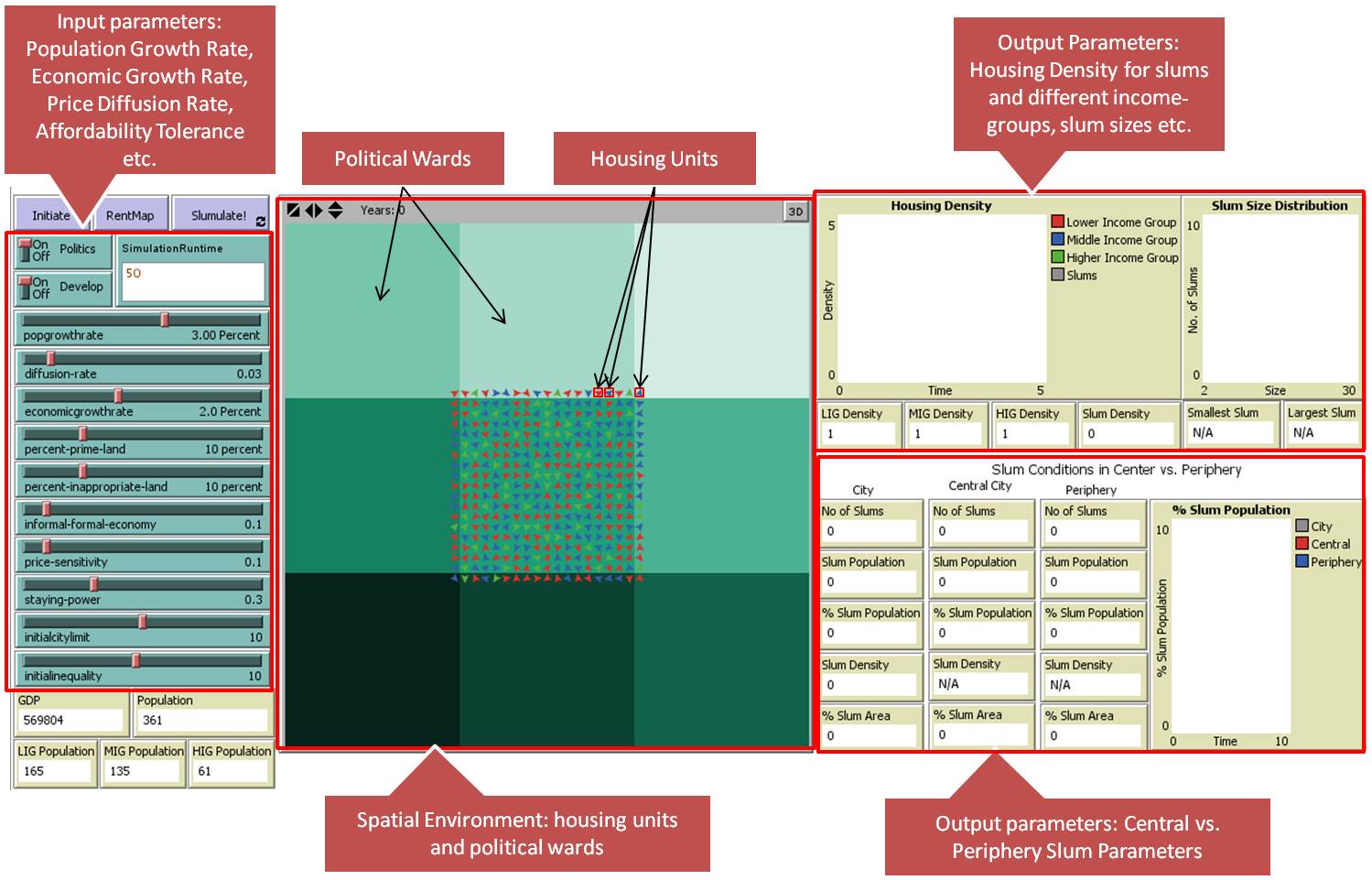
Figure 1. Graphical User Interface for Slumulation

3.12

The physical space in which housing units and political wards are placed is a square grid in a two-dimensional space. The larger squares are political wards that consist of many housing sites represented by the smaller squares. The housing market consists of housing sites in the spatial environment represented by a 51 × 51 square grid resulting into 2601 housing sites. Each square on the grid represents one housing site but it can accommodate a single family or multiple families depending on the number of housing units built on it (e.g. a townhouse, an apartment or a slum). Each housing unit at a given location has a rent associated with it that a household pays in order to occupy it. For simplicity, ownership is not distinguished here and rents are assumed to be equivalent to the mortgage payments for owner-occupiers.

3.13

The city is divided into nine equal political wards, each ward consisting 289 housing sites. The demographics of the wards keep changing as new households appear in the landscape and old households relocate in the simulation process. The effective rent for a given site in a ward is set by politician agents as a function of the dynamically changing proportion of slum dwellers in the ward.

3.14

The color intensity of the smaller squares shows a choropleth of the property rents; the prime properties have the highest rents in the city and are shown in brighter shades of yellow, whereas the inappropriate properties have the lowest rents and are shown in darker shades of yellow as shown in Figure 2. The triangular-shaped objects in Figure 2 represent household agents. The color of each triangle represents the income-class that each agent belongs to; red, blue and green are respectively associated with the agents in low, middle and high-income groups.

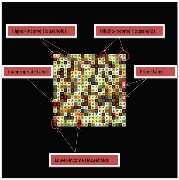
Figure 2. Rent Map Choropleth of the Housing Units Occupied by the Different Income-Groups

Transition and Behavioral Rules

3.15

This section describes transition rules for the various attributes of both the agents and the various spatial entities within Slumulation. The transition rules define how each entity will evolve over time as the simulation progresses. It also describes the behavioral rules for the household agents and its mathematical formulation in the model. The behavioral rules define how agents will respond to the changes in the environment. As in many agent-based models, the transition and behavioral rules are fixed but parameterization of these rules are flexible and user-specified. For example, how the economic growth affects housing prices is specified in the model, but the users can easily alter the value of the economic growth rate to study its impact on the slum formation process.

Housing Prices

3.16

Although the user specifies the initial city size, the percentages of prime and inappropriate sites within the city limits, the actual location and rents for the rest of the housing sites are set randomly by the model. Within the initial city limits, rents are randomly drawn from a normal distribution ranging from the lowest rents for an inappropriate site to the highest rent for a prime site. Outside the initial city limit, the rent is initially set to zero. This assumption is supported by the notion that cities grow and expand into virtually zero priced rural land in the periphery (e.g. Alonso 1964). However, as the simulation progresses, the immediate peripheral land starts gaining value as a response to the anticipated future demand, an effect also seen in the real world.

3.17

During a simulation run, rent may change as a result of the neighborhood effect (captured in diffusion rate below) and economic growth of the city. Rent for each property is calculated at the end of each time period, with the new rent R_it of a property i at time t defined as:

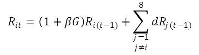
(1)

where d is the diffusion rate defined by user. R_j represents rent at property j in the Moore neighborhood of the property i. G is the economic growth rate and β is the fraction of economic growth attributable to housing market. With this specification in place, rents (R) tend to move towards neighborhood average through price diffusion over time. This process also ensures that periphery is increasingly added into initial city and thus pushes the boundaries of the city outward into previously rural land.

3.18

However, the effective rent ER that a household takes into consideration, can be lower than the actual rent of a property. The effective rent takes into account the decisions from politicians, developers and slum dwellers. Politicians can lower the effective rent of a slum property in the form of subsidy. Developers can add more housing units on an existing site by for example converting a townhouse into apartments. Finally, slum dwellers can increase the number of households living on the same site through illegal squatting. Thus, the effective rent per household, ER_it at site i at time t is given by:

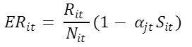
(2)

where N_it is either the number of households in a slum site, or the number of units if the site is held by a developer. In the later case, the units do not have to be occupied. α_jt indicates the proportion of slum population in the ward j at time t (ranging between 0 and 1) which determines the level of subsidy provided to all the slum sites in that ward. S_it is a binary slum-status for the site i at time t (1 if the property is a slum, 0 otherwise).

Household Incomes

3.19

The initial population of households are created within the city limit which is an input specified by the user. At the start of the simulation, each housing site is occupied by a single household, whose income level is set to match the rent of the property that it is occupying. Thus, high income households are located on prime properties and vise versa. Each household is also classified as a low, medium or high income household based on its relative income compared to the average income in the city. Households' income level changes as the simulation progresses and the income-group may also change as a result. The newly formed or migrant households are randomly assigned an income drawn from the distribution of the income in the city at that time. They are also stochastically assigned to either formal or informal labor market in such a way that maintains the predefined proportion of workers in informal sector as reflected by Informality Index.

3.20

At the start of each time period t, a household's income y_it changes based on various factors, namely, its income in previous time period, y_i(t-1), its labor status f_i, and the economic growth rate G. Formally this can be written as:

(3)

where f_i is a binary variable indicating whether the household's labor status is formal or informal. If households are in the formal sector, they can experience full upward income mobility compared to households working in an informal sector who can only experience a fraction (δ) in their upward income mobility.

Residential Mobility

3.21

Newly formed or just arrived households search for an affordable housing unit. They locate at a housing unit that has the rent-payable RP_kt that is less than their capacity to pay C_it (the latter is defined as a pre-determined fraction of their income level). The households already residing on a particular site keep checking that they can continue residing at their present locations by comparing their C_it with the prevailing RP_kt. When the rent-payable exceeds their capacity within a certain fraction of their income, defined by the price-sensitivity RS_it, the households are willing to share the unit with another household of a similar income-group and effectively divide the cost of the rent. RS_it ranges between 0 and 1. The lower price sensitivity results into low tolerance for volatility in rent-payable. The households compare their ability to pay rent with the price-sensitivity adjusted rent-payable when considering the willingness to share. Their transition rule is, remain open to share the unit if:

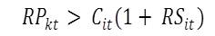
(4)

3.22

Furthermore, there is a limit to keep looking for another household to share the housing unit. The financial staying power, FS_it, determines how long they can stay at an unaffordable housing unit in a hope to get a household to share with them. FS_it ranges between 0 and 1. When the rents cross the limit beyond their financial staying power, they are forced to leave the current place and start searching for an affordable housing unit elsewhere. Their transition rule is, start searching for a house if:

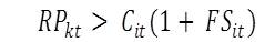
(5)

Population Growth

3.23

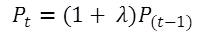
The model is initiated with one household per housing site within the initial city limit specified by the user. The population P changes at the user-specified population growth rate λ during the simulation. The population growth rate is assumed to incorporate both the natural growth and the migration. Thus, the population P_t at time t increases to:

(6)

Economic Growth

3.24

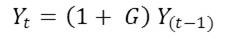
The initial total output of the city Y is the sum of individual incomes of the initial population. Total output changes at user specified economic growth rate G as the simulation progresses. The fraction of this growth-rate (G) is also used for determining appreciation rate of housing prices in the city as specified in Equation 1 earlier. The total output Y_t at time t is thus defined as:

(7)

A Typical Simulation Time-step in Slumulation

3.25

The model is initiated with an initial population of household agents and housing units occupied by them. A user also specifies various parameters such as initial city size, proportion of prime and inappropriate land in the city, population growth rate, economic growth rate, initial income distribution, price diffusion rate for housing and the level of informality of the economy. Each time-step is notionally considered to be one year in the model and the simulation is run for user-specified number of years. Outputs are recorded for each time period. The final spatial representation of the city is preserved as a model output. Figure 3 shows how different entities interact in each time period during the course of a simulation.

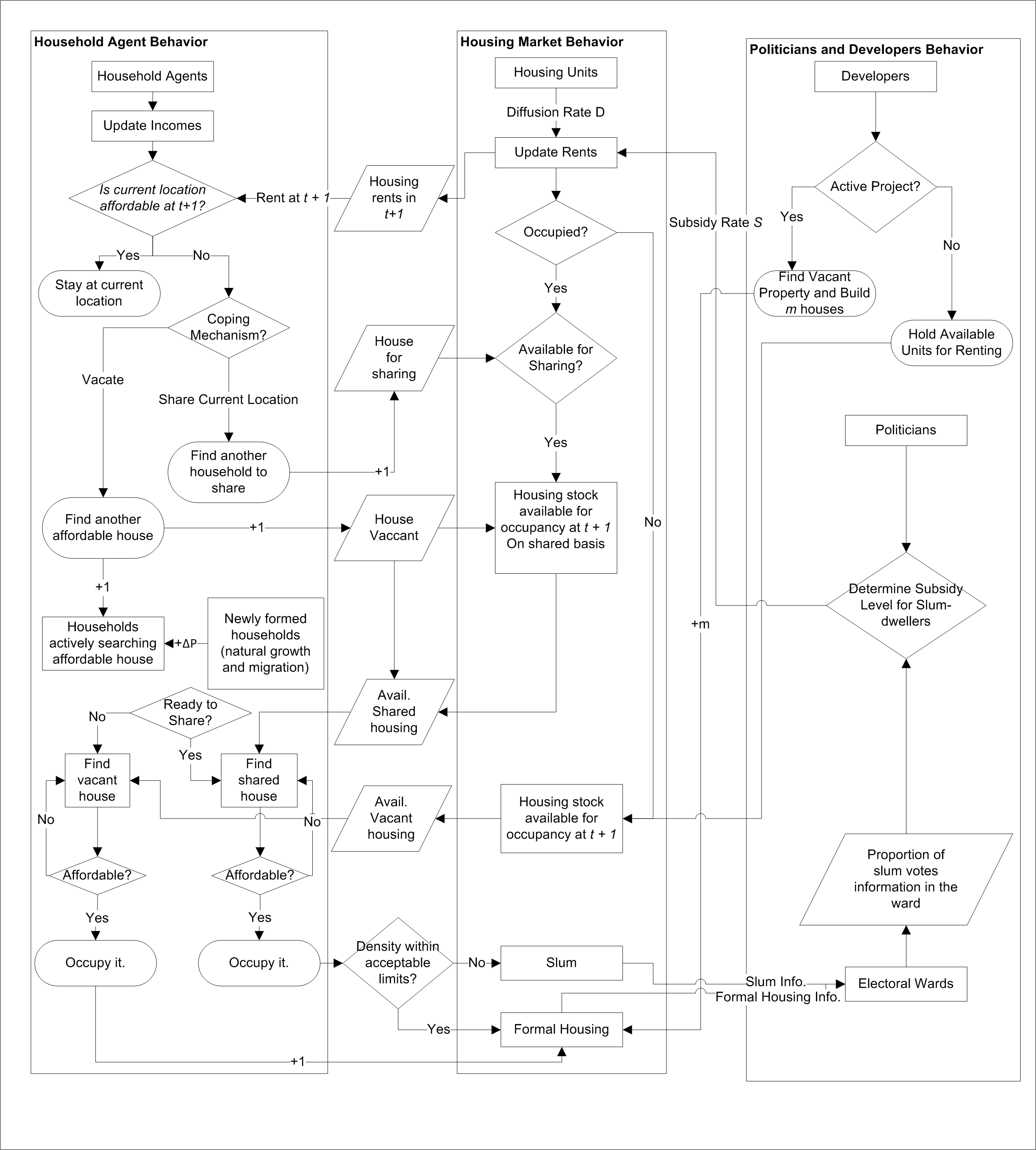
Figure 3. Model Logic and Interactions Between Different Entities During the Course of a Simulation

3.26

While model-wide temporal changes such as agents' income and housing prices are updated synchronously at the end of each time-step, household relocation and the resulting change in newly occupied housing sites (i.e. occupancy status, number of occupants etc.) are updated asynchronously. All active households who are searching for a new location are relocated within the time-step but they are initiated one by one in a randomized order. During the simulation, each vacated housing site is occupied by a newly created developer whose principal role is to create new housing units on that site and hold the vacant units for future occupancy by households. Developer agents exit once all newly created units are occupied.

Outcome Measures

3.27

We used the fifth criteria of the UN-Habitat (2006) definition of a slum household i.e. insufficient living area to declare a housing site as a slum. We chose this criteria primarily because it is the only criteria that reflects household's choice. For example, households may influence the decisions pertaining to the first two criteria at a particular location (i.e. lack of water and sanitation), but these are primarily the outcomes of large-scale infrastructure investment decisions by public authorities and are usually taken at neighborhood or even larger area scale. The third and fourth criteria of the slum definition, namely, secured tenure and durable structure, can be assumed to be directly reflected in prevailing housing prices and rents (e.g. a housing unit with a durable structure will be priced higher than that of one with a temporary structure). Housing density is the only parameter that collectively "emerges" from individual household's location choices and interaction with other households such as sharing behavior. The housing density parameter provides an outcome measure resulting purely from household behavior and hence it is important from the perspective of building an agent-based model. We intend to incorporate the other four criteria as part of spatial environment in future versions of Slumulation.

3.28

In the real world, the insufficient living space criteria is operationalized as three or more persons per room to declare a household as a slum household (UN-Habitat 2006). We implement this criteria in our model by declaring a housing site as a slum if it is occupied by more households than the number of units available on that site, as we do not model housing units at the room level and households at the individual level. However, our simplified measure captures the essence of the UN-Habitat criteria. Once a housing site is classified as slum and non-slum, a series of indicators are calculated to study the overall outcome of the model. Particularly, we report average slum density, number of slums, percentage slum population, percentage area under slums, both for the center and the periphery separately as well as the average for the entire city. We also create graphs showing density for slums as well as for all three income groups over time. Similarly, we also report slum size distribution for the entire city as shown in Figure 1.

Model Verification

4.1

Each input parameter of Slumulation was varied to understand its effect on the simulation outcome, in particular the final patterns of housing density (for slums as well as for other income-groups) and the percentage of slum population in the city. We refer to verification as a means of ensuring that the implemented model matches its design (North and Macal 2007), a process that involves checking that the model behaves as expected. Such verification, is sometimes referred to as testing the "inner validity" of the model (Brown 2006). First, we ran the model with the input parameter values shown in Table 1. Some of the values chosen as default were those typically found in the cities in developing world. For example, the population in Indian cities grew at 3% annually on an average between 1991 and 2001 (Census of India 2001). However, generalizable empirical data on certain parameters are often not collected or publicly available. In such cases, we have taken our informed judgment in choosing the values.

Table 1: Input Parameters for a Typical Simulation Run
Input Parameters	Values
Population Growth Rate (λ)	3.0%
Economic Growth Rate (G)	2.0%
Housing Price Growth Rate Fraction (β)	0.5
Initial Prime-land	10.0%
Initial Inappropriate-land	10.0%
Neighborhood Price Diffusion Rate	3.0%
Price-Sensitivity (RS)	0.1
Financial Staying Power (FS)	0.3
Informality Index	0.7
Income Growth Rate Fraction for Informal Sector (δ)	0.1
Fraction of Income available for Housing Rent (C)	0.3
Initial City Population	361
Politics	On
Development	On
Initial Inequality	10
Simulation Run Time (T)	50

4.2

The simulation experiment was run for 50 time periods (years) and was repeated 100 times. We have chosen 50 time-steps as it represented a long enough simulation time but readers interested in exploring this further e.g. for longer time period, are encouraged to run the model which is available at http://css.gmu.edu/Slums. However, it needs to be noted that the simulation stops if physical space runs out while households are searching for a new location which limits this model's capacity to test population growth scenario to an extent. Choosing a smaller city-size as the initial condition can help to partially overcome this limitation. We ran the model with smaller initial city-size for 150 time periods and found that some of the outcome parameters such as overall slum percentage stabilizes after approximately 40 time periods and roughly remains at that level for the remainder of the run. It should also be noted that our approach, by design, is to make this model dynamic and hence all parts of the system never reaches an equilibrium state per se. For example, locations of slums spatially alters over time. Agent population also keeps growing and hence the model could not possibly reach an equilibrium state in the strict sense.

4.3

Figure 4 illustrates a typical simulation run, where the maps show the spatial distribution of the rents and the charts show the evolution of housing density for each income-group, and the % slum population. As is visible from Figure 4d, housing density increases for both slums and the lower-income group (LIG) from the beginning of the simulation suggesting inability of the poor to keep up with the rising housing rents. Whereas, housing density for the higher-income group (HIG) virtually remains the same throughout the simulation period, suggesting no economic hardship on housing front for the high-income group. However, the middle-income group (MIG) also experience hardship when faced with the rising housing rents, suggesting that the middle-income group opts for high-density housing types (e.g. apartments) over single family-homes.

4.4

The maps of the rent gradients and locations of the various income-group households in Figure 4 suggest another story. The lower-income group tends to occupy the peripheral housing sites because rents are comparatively low in the periphery. This pattern is similar to the patterns observed in the developing world cities, where such peripherization of urban slums is documented, for example, in several Latin American cities (see Barros 2005). However, lower-income households are also occupying some of the most expensive housing sites in the later part of the simulation. These properties are made affordable by sharing extensively which results in high densities. The densification is dominant in the central ward because the already high proportion of slum households benefit from the subsidy provided by politicians. This result is also in confirmation with the politics of slums. For example, Dharavi in the city of Mumbai occupies a site that would be highly priced in formal market but residents have not been evicted despite several proposals in the past (Mahadevia and Narayan 1999).

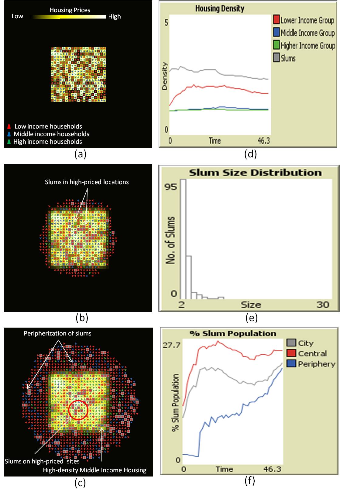
Figure 4. Typical simulation outputs: initial conditions (a), housing rent gradient and occupancies at time t = 25 (b), and t = 50 (c). Housing density for slums and other income-groups (d) slum size distribution at t = 50 (e), and % slum population over time (f)

4.5

Table 2 highlights average slum population, number of slums and slum density in different regions of the city from multiple simulation runs using the input parameters from Table 1. Our exploratory model produces housing conditions that are observed in some cities in developing countries. For instance, in the city of Mumbai, the densest slum, Dharavi, is 11 times as dense as the city's average density (Mukhija 2001;Rao 2007). The densest slum in our simulation is 7.3 times denser than the city's average density, while the proportion of slum population in the simulation is 19.7%, which are plausible results. However, individual cities vary dramatically in slum prevalence (UN-Habitat 2008) and hence the goal of this model is not to produce the actual percentage of slums for a particular simulated city. Rather its aim is to produce outcomes for a wider range of instances and therefore it should be sensitive to input parameters as discussed in subsequent model experiments section. In the simulation above, slums have a higher density in the central electoral ward (2.69) compared to peripheral wards (2.30 on average for 8 peripheral wards) as shown in Table 2. This trend is indicative of higher prices prevailing in central part of the city combined with households' higher preferences to live closer to the center. Furthermore, the high-density housing of middle-income households is also visible in the central part of the city suggesting the concentration of high-rise/high-density apartments. Developers within the model play a key role in this densification process by financing and replacing single-family housing with multi-family apartments, thereby reducing effective rent per household.

Table 2: Mean of Key Output Parameters at t = 50 for 100 simulation runs (Numbers in parenthesis indicate standard deviation)
Output Parameters	City	Center	Periphery
Percent Slum Population	19.0 (0.3)	16.8 (0.4)	19.7 (0.4)
Percent Area under Slums	10.1 (0.2)	8.5 (0.2)	10.6 (0.2)
Slum Density	2.30 (0.01)	2.69 (0.04)	2.21 (0.01)
Number of Slums	125 (2)	24 (1)	101(2)

4.6

In the next phase of our model verification, we configured various model components in many different ways to study the impact of selected model specifications. For example, we ran the model with and without politician and developer agents. All other parameters were kept the same as our control case, reported in Table 1. We also verified that the presence or absence of each component impacts the results in a plausible manner. As seen in Table 3, when politician agents are deactivated, slum population in the central ward decreases from 16.0% to 13.9% (or 24.8% to 22.0% when development is off). This trend is indicative of slum-dwellers' inability to resist economic forces (reflected in increasing housing rents) in absence of subsidy by the politicians. Similarly, when developers are turned inactive, slums increase all over the city. This outcome is indicative of developers' central role in creating dense housing types in highly priced sites and thus making housing affordable at desirable locations. In absence of such formal densification, one would expect the rise in slum population i.e. informal divisions of properties to make them more affordable.

Table 3: Impact of Politics and Development Component on Model Outcomes (Numbers in parenthesis indicate standard deviation)
Output Parameters		Politics ON Development ON (Base)	Politics OFF Development ON	Politics ON Development OFF	Politics OFF Development OFF
Percent Slum Population	City	19.2 (0.3)	18.7 (0.2)	24.4 (0.4)	25.3 (0.2)
	Center	16.0 (0.4)	13.9 (0.3)	24.8 (0.5)	22.0 (0.4)
	Periphery	20.3 (0.3)	20.2 (0.3)	24.2 (0.4)	26.1 (0.3)
Percent Area under Slums	City	10.3 (0.2)	10.1 (0.1)	12.1 (0.2)	12.5 (0.1)
	Center	8.3 (0.2)	7.3 (0.1)	11.2 (0.2)	9.6 (0.2)
	Periphery	11.0 (0.2)	11.0 (0.2)	12.3 (0.2)	13.3 (0.1)
Slum Density	City	2.26 (0.01)	2.28 (0.01)	2.35 (0.01)	2.37 (0.01)
	Center	2.54 (0.04)	2.62 (0.04)	2.62 (0.03)	2.66 (0.03)
	Periphery	2.20 (0.01)	2.20 (0.01)	2.28 (0.01)	2.31 (0.01)
Number of Slums	City	128 (2)	126 (2)	158 (2)	163 (1)
	Center	24 (1)	21 (1)	32 (1)	28 (1)
	Periphery	105 (1)	105 (2)	125 (2)	135 (1)

4.7

We have also verified the model by changing several other components to study their impacts on model outcomes. For example, we tested the model for two different types of search processes when a household considers relocation: i) prefer locations near the current location, or ii) prefer locations close to the center. While the search process might have an impact on individual households' residential mobility patterns, we found that the aggregate result for various slum measures such as the percentage of slum population, slum density and percent slum area, were not very sensitive to the choice of search process.

4.8

Similarly, we also tested the model sensitivities of several different specifications of the model whose outputs are not reported in this paper for brevity. For example, we tested how the rule to determine availability of housing units in a slum changed the model outcomes. In one scenario we made a slum site available for further occupancy even if the slum site is within the affordability range of the current residents. Alternatively, as it is implemented in the model presented here, it can be restricted from potential residents when all the original residents can afford it. This choice of specification on availability affects some of the outcome measures. For example, the number of slums are less when we make slums available for further occupancy irrespective of current residents affordability criteria. However, these are common dilemmas faced in agent-based modeling. As a guiding principle, we have chosen to incorporate rules that make more intuitive and logical sense and ones that are close to the real world.

Simulation Experiments

5.1

Once confidence was gained pertaining to inner workings of the model, the parameter space was explored by varying various input parameters, one at a time. The configuration shown in the previous section (Table 1) acts as our base scenario for these parameter sweeps. We tested several mechanisms; that of population growth rate, economic growth rate, the initial proportion of prime and inappropriate land and finally the mix of formal and informal employment in the city. Each simulation experiment was run with three different values for 50 time periods and was repeated 100 times. The simulation outputs presented below are means of these 100 runs for each scenario. Standard deviations were within 2 to 4% range for all of these parameters and hence not reported for clarity. We first sketch out our rationale for choosing these scenarios before presenting the results for each scenario below.

Population Growth Rate

5.2

More and more people are living in cities and this trend is expected to continue in the near future (United Nations 2007) with unprecedented numbers living in slums (UN-Habitat 2003). In this experiment, we test how the population growth in the city could impact the slum conditions. Population growth rate was set to 2.0%, 3.0% (base scenario) and 4.0%. We observed that higher population growth (4%) leads to higher percentage slum population (27.9%) whereas slower population growth leads to lower percentage slum population (13.0%) as shown in Table 4. Of note is the non-linear relationship with population growth.

Table 4: Impact of Population Growth Rate on Model Outcomes
Output Parameters		Population Growth Rate 2.0 %	Population Growth Rate 3.0 % (Base)	Population Growth Rate 4.0 %
Percent Slum Population	City	13.0	19.0	27.9
	Center	14.2	16.3	12.1
	Periphery	12.1	20.0	30.5
Percent Area under Slums	City	7.4	10.1	14.3
	Center	8.1	8.2	4. 9
	Periphery	7.0	10.7	15.9
Slum Density	City	2.24	2.30	2.44
	Center	2.43	2.68	3.12
	Periphery	2.09	2.21	2.41
Number of Slums	City	54	126	283
	Center	23	24	14
	Periphery	31	102	269

5.3

The higher population growth rate also results in a greater number of slums as opposed to densification of existing slums. The resulting slum formation pattern shows a higher number of peripheral slums as highlighted in Table 4. This is a hypothesis worth testing using real world data, whether the higher pace of population growth results into higher peripherization rather than higher densities. It seems that exploring new location is preferred over exploiting existing locations during the rapid population growth period. For example, historically, cities have expanded physically during period of increased migration, and the densification process took place much later in the evolution of a city (Sudhira et al. 2004). Rapid urbanization is often cited as a factor in the slum formation process but it is often less understood how it plants seeds for future slum formations. It seems from this experiment that future slum locations are identified on the new frontier by new migrants during the rapid population growth phase of a city.

Economic Growth Rate

5.4

Economic growth has a large impact on why people move to cities (UN-Habitat 2010). For example, Mumbai grew exponentially by attracting migrants from rural India as it added new manufacturing jobs (Yedla 2003). In order to study how economic growth impacts on the formation of slums, we tested three different values for the economic growth rate: 2.0% (base scenario), 3.5% and 5% while all other parameters were kept constant. The results are summarized in Table 5.

Table 5: Impact of Economic Growth Rate on Model Outcomes
Output Parameters		Economic Growth Rate 2.0% (Base)	Economic Growth Rate 3.5%	Economic Growth Rate 5.0%
Percent Slum Population	City	19.2	16.8	15.9
	Center	16.3	13.5	10.9
	Periphery	20.2	18.0	17.5
Percent Area under Slums	City	10.2	9.0	8.3
	Center	8.2	6.6	4.7
	Periphery	10.9	9.7	9.4
Slum Density	City	2.30	2.28	2.29
	Center	2.67	2.67	2.97
	Periphery	2.21	2.19	2.19
Number of Slums	City	127	112	104
	Center	24	19	14
	Periphery	103	93	91

5.5

The proportion of population living in slums decreases from 19.2 to 15.9%. However, there is no spatial implication as it is evident from the reduction experienced in both center and periphery. The density of slums remains unaffected. It is evident from this experiment that the higher economic growth reduces the number of slums from 127 to 104. One again, the number of slums reduces both in center and periphery thus indicating the absence of any spatial implication of economic growth.

Initial Land Supply Conditions

5.6

Cities are historically endowed with land parcels that are considered prime in the sense that they have easy access to jobs, recreation, social amenities and have adequate infrastructure services. Whereas some land parcels are naturally unsuitable for development, for example, hazardous sites such as riverbeds, sites near polluting industries or landfills, sites with poor accessibility from major transportation networks or inadequately serviced in terms of water and sanitation etc. We test how endowment of higher or lower proportion of prime or inappropriate land parcels in a city affect the slum formation process. The initial proportion of prime-land was simulated for three test values: 10% (base value), 20% and 30% while all other parameters were kept constant. The results are shown in Table 6.

Table 6: Impact of Prime-land on Model Outcomes
Output Parameters		Prime Land 10% (Base)	Prime Land 20%	Prime Land 30%
Percent Slum Population	City	19.0	19.0	18.6
	Center	15.7	14.5	13.4
	Periphery	20.1	20.4	20.3
Percent Area under Slums	City	10.3	10.1	9.9
	Center	8.2	7.3	6.6
	Periphery	10.9	11.0	10.9
Slum Density	City	2.27	2.28	2.26
	Center	2.59	2.67	2.64
	Periphery	2.20	2.20	2.20
Number of Slums	City	127	126	125
	Center	24	21	19
	Periphery	104	105	106

5.7

A notable outcome from this experiment is a reduction in the percentage of slums, percentage area under slums and an increase in slum density in the central part of the city. There is also a higher proportion of prime-land in the initial central city that lower-income households cannot afford. Lower-income households accordingly face the supply constraint which results into the peripherization of slums or higher densities in relatively lower number of existing slums in the central city. Higher prices are also observed due to the neighborhood effect (sites near prime-land observes price appreciation over time). It would be worth investigating this result with respect to real world cities to see if there is any path dependencies in the slum formation rate based on initial land conditions.

5.8

In the next experiment, we investigated the impact of inappropriate land supply. The supply of prime land was kept constant at the base scenario (10%), but the percentage of inappropriate land was changed to three different test values: 10% (base scenario), 20% and 30%. The results are shown in Table 7.

Table 7: Impact of Inappropriate Land Supply on Model Outcomes
Output Parameters		Inappropriate Land 10% (Base)	Inappropriate Land 20%	Inappropriate Land 30%
Percent Slum Population	City	18.9	18.9	18.9
	Center	16.3	16.4	17.6
	Periphery	19.8	19.8	19.2
Percent Area under Slums	City	10.2	10.1	10.0
	Center	8.6	8.3	8.8
	Periphery	10.7	10.7	10.4
Slum Density	City	2.27	2.30	2.31
	Center	2.56	2.71	2.82
	Periphery	2.19	2.21	2.18
Number of Slums	City	127	125	124
	Center	25	24	25
	Periphery	102	102	99

5.9

A higher initial supply of inappropriate land in the center results into a higher slum population in the center as well as higher densities in those slums. It is interesting that while the overall number of slums in the central city actually declines, the slum density increases indicating growth of existing slums originally sited on inappropriate locations. This result has analogies with what we find in real world cities e.g. Dharavi, a largest slum in Mumbai, which was populated with large influx of migrants in 1920s (Clothey 2006) on a land parcel that was inappropriate for development (for example, there were no roads in Dharavi and it was an island within marsh land). The slum persists even today despite that formal development has taken place in all surrounding areas (MCGM 2005). Similar patterns are found elsewhere e.g. landfill sites, such as those in Manila, Philippines (Abad 1991).

Informal-formal Sector Mix

5.10

It has been noted in literature (e.g. Mitra 2008;Tamaki 2010) that the people employed in informal sector cannot expect much upward mobility in their incomes compared to those employed in the formal sector. To test this, we explore how the percentage of slum population changes with different mixes of formal and informal sectors in the city economy. Three test values of the formality index were simulated: 0.1 (base scenario, i.e. the majority of the workforce is in the formal sector), 0.4 and 0.7 (i.e. the higher proportion of the workforce is increasingly working the informal sector) while all other parameters were kept constant. The results are shown in Table 8. Of note is that both the overall densities and slum population increases as economy has higher informality. This indicates that a greater number of people working in the informal sector increases the income inequalities but does not result into affordable housing available for lower income groups and hence results into higher slum population.

Table 8: Impact of Informality on Model Outcomes
Output Parameters		Informality Index 0.1 (Base)	Informality Index 0.4	Informality Index 0.7
Percent Slum Population	City	17.0	17.4	18.2
	Center	12.6	13.6	15.6
	Periphery	18.4	18.6	19.1
Percent Area under Slums	City	8.9	9.2	9.8
	Center	6.5	6.9	8.0
	Periphery	9.6	9.8	10.3
Slum Density	City	2.22	2.24	2.27
	Center	2.42	2.49	2.62
	Periphery	2.19	2.19	2.19
Number of Slums	City	116	118	121
	Center	19	20	23
	Periphery	98	98	99

5.11

The results presented here are based on experiments that vary one parameter at a time but many other type of experiments could be run using Slumulation. For example, varying multiple parameters such as higher formalization combined with higher economic growth. Similarly, all parameters could be changed in order to find a set of parameter values that would reduce the number of people living in slums (or result in no slums).

Discussion and Further Work

6.1

This paper has attempted to build an exploratory ABM called Slumulation, to model slum formation using our existing understanding of urbanization processes, urban morphology, housing markets, and migrants' behavior within a spatial ABM framework. Specifically, the model adds to the small but growing body of literature that uses agent-based models to aid our understanding of slum formation. Slums are results of a combination of conditions present at various spatial scales, coupled with the interplay of different actors, ranging from the individual household to local politicians and developers, all of which influence the emergence or persistence of the slums. We believe that our approach to model slum formation and expansion is unique as it explicitly incorporates political behavior with regard to political protection of slum communities by explicitly modeling politicians as agents. Similarly, a role of developers who transform low-density housing into high-density housing is modeled to analyze the impact on both formal housing market growth and slum formation. Agent-based models of slum formation often ignore these two important actors and their roles in slum formation and expansion process. Incorporating these agents also required our model to be multi-scalar which is then lacking in prior modeling efforts with regard to slums.

6.2

Our model suggests that higher protection of slum-dwellers in the form of subsidies in lieu of slum votes results into slums with high densities. While peripherization of slums slows down as the formation of new slums decreases, several slums persist on the prime-land for a longer amount of time in the center. Virtually, none of the slum households get evicted despite the rising prices in the central city when politician agents are active. It should be noted that we do not claim that slums are more likely in democratic societies. We only show that political representation of slum-dwellers in the form of voting rights allow them to resist economic forces by building an electorate. In simulating cities where slum-dwellers are not given voting rights, our model could easily be adapted by turning off the politics provided as a switch in the model interface as we demonstrated above. The developers provide a central role in converting low-density middle-income neighborhoods into high-density middle-income neighborhoods. This central function of developers releases the upward pressure on real estate. Increased density provided in the formal manner results into better housing conditions despite higher densities.

6.3

Moreover our experiments suggest that economic growth and formal-infomal mix has a direct impact on slum formation. It seems that economic growth alone cannot alleviate slum issues in developing world cities. It is necessary to increase formality which has a two-pronged effect: i) reducing income inequality and ii) housing prices are within affordability limits for all sections of society. These effects are well captured in the model and suggest that economic growth combined with reduced inequality may reduce slum growth in developing world. Similarly, the fast pace of urbanization is often considered a driving force for slum formation. However, our experiments suggest that cities expand and increase the sprawl but do not necessarily increase housing densities beyond acceptable limits during a rapid population growth phase.

6.4

The purpose of this model is explanatory and it simply explores theories and generates new hypotheses. However, future work will attempt to model an actual metropolitan area from the developing world (such as Mumbai, India) and take it to a "Level 2" model in terms of Axtell and Epstein's (1994) classification system. In order to do so, we will need to build on the empirical works of slum researchers who explore issues relating to: management of informal settlements with the aid of geographical information systems (e.g. Sliuzas et al. 2004); housing transformation (e.g. Sheuya 2004); as well as issues pertaining to informal land management (e.g. Kombe and Kreibich 2000).

6.5

Also, for simplicity, we assumed a normal distribution with respect to income for initial population. While, a normal distribution is a conservative approach, in future work we will try more realistic income distributions such as log-normal and exponential. We believe that such distributions are closer to reality and it will help us to advance future versions of our model to more closely match the real world. Nonetheless, the model did generate "real" world patterns of slum formation and sustenance over space and time, offering "candidate explanations" (Epstein 1999) for the emergence of observed patterns.

6.6

Another direction of the model extension is to incorporate more complex behaviors and interactions. For example, it might be interesting to explore the competition between the developers for the sites. However, this would involve developing a more complicated land market mechanism than that currently implemented in the model. The work of Filatova et al. (2009) could be a good starting point for this. Similarly, the competition between two political parties could be introduced that would work in both directions rather than simply protecting the poor (Kim 2011; Muis 2010). The role of government is also important in developing new green-field sites by providing infrastructure, which is currently absent in the model. The economic growth and formal-informal mix determines the level of budget available for such a development and may become more important parameters once the role of government is introduced in supply of serviced land. Data on some of these input parameters might not be available readily for cities in developing countries. However, one can hope that our model may precede and guide empirical work in this area as is the case with many other theoretical and exploratory works (Epstein and Axtell 1996).

6.7

As Wilson (2000) writes, understanding cities represent one of the greatest challenges of our time. As more than a third of the world's population currently live in slums (UN-Habitat 2003), we believe that slums represent a great challenge. Agent-based modeling is an useful tool to study questions relating to how slums come into existence, how do they expand, and which processes may make some slums disappear. We believe this is especially true because agent-based modeling is inherently dynamic and focuses on individual behavior that is manifested in the formation of slums.

Acknowledgements

The authors would like to thank the National Science Foundation and its Geography and Spatial Sciences Program (NSF-BCS-1225851). In addition the authors would also like to thank the three anonymous reviewers for their detailed and helpful reviews.

Notes

¹ Slumulation currently only tackles the spatial scale. However, we note that different temporal scales play a role and we are investigating how this can be incorporated into the model. For example, residential movement occurs at a different temporal scale than that of political elections and the development of land.

References

ABAD, R.G. (1991). Squatting and Scavenging in Smokey Mountain. Philippine Studies. Vol. 39. No. 3: 263-286.

ALONSO, W. (1964). Location and Land Use: Toward a General Theory of Land Rent. Harvard University Press, Cambridge, MA. [doi:10.4159/harvard.9780674730854]

AUGUSTIJN-BECKERS, E. Flacke, J. and Retsios, B. (2011). Simulating Informal Settlement Growth in Dar es Salaam, Tanzania: An Agent-based Housing Model. Computers, Environment and Urban Systems, 35(2): 93-103. [doi:10.1016/j.compenvurbsys.2011.01.001]

AXTELL, R and Epstein, J. (1994) Agent-based Modeling: Understanding Our Creations. The Bulletin of the Santa Fe Institute, Winter 1994, pp. 28-32.

BARROS, J. (2005), Simulating Urban Dynamics in Latin American Cities. In Atkinson, P., Foody, G., Darby, S. and Wu, F. (eds.), GeoDynamics, pp. 313-328. CRC Press, Boca Raton, FL.

BATTY, M. (2005). Cities and Complexity: Understanding Cities with Cellular Automata, Agent-Based Models, and Fractals. The MIT Press, Cambridge, MA.

BENENSON, I. and Torrens, P.M. (2004). Geosimulation: Automata-Based Modelling of Urban Phenomena. John Wiley & Sons, London, UK. [doi:10.1002/0470020997]

BHARUCHA, N. (2011). State 'Gifts' 6 Builders 500 Acres of Slum Land. Times of India (1st February, 2011). http://articles.timesofindia.indiatimes.com/2011-02-01/mumbai/28365366_1_slum-dwellers-slum-cluster-slum-land archived at: http://www.webcitation.org/60iVaM24M

BROWN, D.G. (2006). Agent-Based Models. In Geist, H. (ed.) The Earth's Changing Land: An Encyclopaedia of Land-Use and Land-Cover Change. pp. 7-13. Greenwood Publishing Group, Westport, CT.

BURGESS, E.W. (1927). The Determinants of Gradients in the Growth of a City. Publications of the American Sociological Society. 21: 178-84.

CENSUS OF INDIA (2001). Census Data Products available from Office of the Registrar General and Census Commissioner, New Delhi, India.http://censusindia.gov.in/ [Accessed on January 11th, 2012].

CHEGE, M. (1981). A Tale of Two Slums: Electoral Politics in Mathare and Dagoretti. Review of African Political Economy, 20(1): 74-88. [doi:10.1080/03056248108703457]

CLARKE, K.C., Hoppen, S. and Gaydos, L.J. (1997). A Self-Modifying Cellular Automaton Model of Historical Urbanization in the San Francisco Bay Area. Environment and Planning B, 24(2): 247-261. [doi:10.1068/b240247]

CLOTHEY, F.W. (2006). Ritualizing on the Boundaries: Continuity and Innovation in the Tamil Diaspora. University of South Carolina Press, Columbia, SC.

EPSTEIN, J. M., & Axtell, R. (1996). Growing Artificial Societies: Social Science from the Bottom Up. Complex adaptive systems. Washington, D.C: Brookings Institution Press.

EPSTEIN, J.M. (1999). Agent-Based Computational Models and Generative Social Science. Complexity, 4(5): 41-60. [doi:10.1002/(SICI)1099-0526(199905/06)4:5<41::AID-CPLX9>3.0.CO;2-F]

FILATOVA, T., Parker, D. and van der Veen, A. (2009). Agent-Based Urban Land Markets: Agent's Pricing Behavior, Land Prices and Urban Land Use Change. Journal of Artificial Societies and Social Simulation, 12(1), 3 available at https://www.jasss.org/12/1/3.html.

GLAESER, E. and SHLEIFER, A. (2003). The Curley Effect: The Economics of Shaping the Electorate. The Journal of Law, Economics, & Organization, 21(1): 1-19. [doi:10.1093/jleo/ewi001]

GRIMM, V. (2002). Visual Debugging: A Way of Analyzing, Understanding, and Communicating Bottom-up Simulation Models in Ecology. Natural Resource Modeling, 15(1): 23 - 38. [doi:10.1111/j.1939-7445.2002.tb00078.x]

HEPPENSTALL, A.J., Crooks, A.T., Batty, M. and See, L.M. (eds.) (2011). Agent-based Models of Geographical Systems. Springer.

JANSON, C. (1980), Factorial Social Ecology: An Attempt at Summary and Evaluation. Annual Review of Sociology, 6: 433-456. [doi:10.1146/annurev.so.06.080180.002245]

JOHNSTON, R.J. (1971). Some Limitations of Factorial Ecologies and Social Area Analysis. Economic Geography, 47(3): 314-323. [doi:10.2307/143213]

KIM, S. (2011). A Model of Political Judgment: An Agent-Based Simulation of Candidate Evaluation. Journal of Artificial Societies and Social Simulation, 14(2), 3 available at https://www.jasss.org/14/2/3.html.

KOMBE, W.J. and Kreibich, V. (2000). Reconciling Informal and Formal Land Management:: An Agenda for Improving Tenure Security and Urban Governance in Poor Countries. Habitat International, 24(2): 231-240. [doi:10.1016/S0197-3975(99)00041-7]

FIELDS, G.S. (2011). Labor Market Analysis for Developing Economies. Labour Economics.Vol. 18. Supplement. 1: s16-s22. [doi:10.1016/j.labeco.2011.09.005]

MAHADEVIA, D. and Narayan, H. (1999). Shanghaing Mumbai - Politics of Evictions and Resistance in Slum Settlements. Center for Development Alternative: Working Paper 7, Ahmedabad, India.

MCGM (2005). Mumbai City Development Plan: 2005-2025. Mumbai: Municipal Corporation of Greater Mumbai, Mumbai, India.

MHUPA (2010). Status Note on Rajiv Awas Yojana. Ministry of Housing and Urban Poverty Alleviation, Government of India, New Delhi. available at: http://mhupa.gov.in/W_new/NOTE_RAJIV_AWAS_YOJANA.pdf

MILLS, E.S. (1972). Studies in the Structure of the Urban Economy. Johns Hopkins Press, Baltimore, MD.

MITRA, A. (2008). Social Capital, Livelihood and Upward Mobility, Habitat International, 32(2): 261-269. [doi:10.1016/j.habitatint.2007.08.006]

MUIS, J. (2010). Simulating Political Stability and Change in the Netherlands (1998-2002): an Agent-Based Model of Party Competition with Media Effects Empirically Tested. Journal of Artificial Societies and Social Simulation, 13(2), 4 available at https://www.jasss.org/13/2/4.html.

MURRAY, M. (2010). City of Extremes: The Spatial Politics of Johannesburg. Duke University Press.

MUKHIJA, V. (2001). Enabling Slum redevelopment in Mumbai: Policy Paradox in Practice, Housing Studies, 16(6): 791-806. [doi:10.1080/02673030120090548]

MUMFORD, L. (1961). The City in History: Its Origins, Its Transformations, and Its Prospects. Houghton Mifflin Harcourt, New York, NY.

MUTH, R. (1969). Cities and Housing. University of Chicago Press, Chicago, IL.

NEUWIRTH, R. (2005). Shadow Cities: A Billion Squatters, A New Urban World. Routledge, New York, NY.

NORTH, M.J. and Macal, C.M. (2007). Managing Business Complexity: Discovering Strategic Solutions with Agent-Based Modelling and Simulation. Oxford University Press, New York, NY. [doi:10.1093/acprof:oso/9780195172119.001.0001]

O'SULLIVAN, D. (2009). Changing Neighborhoods - Neighborhoods Changing: A Framework for Spatially Explicit Agent-based Models of Social Systems. Sociological Methods and Research, 37(4): 498-530. [doi:10.1177/0049124109334793]

PARTHASARTHY, G. and Pothana, V. (1981). Congress(I) and the Poor. Economic and Political Weekly, 16(37): 1491.

RAO, V. (2007). Proximate Distances: The Phenomenology of Density in Mumbai. Built Environment, 33(2): 227-248. [doi:10.2148/benv.33.2.227]

ROY, A. and Alsayyad, N. (eds.) (2004). Urban Informality: Transnational Perspectives from the Middle East, Latin America, and South Asia. Lexington Books, Lanham, MD.

SCHELLING, T.C. (1971). Dynamic Models of Segregation. Journal of Mathematical Sociology, 1(1): 143-186. [doi:10.1080/0022250X.1971.9989794]

SETHURAMAN, S.V. (1976). The Urban Informal Sector: Concept, Measurement and Policy. International Labour Review. Vol. 114. No. 1: 69-81.

SHEUYA, S. (2004). Housing Transformation and Urban Livelihoods in Informal Settlements The Case of Dar es Salaam, Tanzania. Spring Research Series, No. 45, Dortmund, Germany.

SHEVKY, E. and Bell, W. (1955). Social Area Analysis: Theory, Illustrative Application and Computational Procedures. Stanford University Press, Palo Alto, CA.

SIETCHIPING, R. (2004). A Geographic Information Systems and Cellular Automata-based Model of Informal Settlement Growth. PhD thesis, School of Anthropology, Geography and Environmental Studies, The University of Melbourne, Melbourne, Available at http://repository.unimelb.edu.au/10187/1036.

SINGH, G. (1986). Bombay Slums Face Operation Demolition. Economic and Political Weekly, 21(16): 684-687.

SLIUZAS, R.V., Ottens, H. and Kreibich, V. (2004). Managing Informal Settlements: A Study Using Geo-information in Dar es Salaam, Tanzania. Ph.D. Thesis, Utrecht University, Enschede, Netherlands, Available at http://www.itc.nl/library/Papers_2004/phd/sliuzas.pdf.

SUDHIRA, H.S., Ramachandra, T.V. and Jagadish, K.S. (2011). Urban Sprawl: Metrics, Dynamics and Modelling using GIS. Observation and Geoinformation, 5(1): 29-39. [doi:10.1016/j.jag.2003.08.002]

TAMAKI, E. (2010). Occupational Change and Upward Mobility of Low-Income Residents in Bangkok. Southeast Asian Studies, 48(2): 131-154.

TIMES OF INDIA (2009). UPA's Target - A Slum Free India in 5 Years, Times of India (5th June,2011), Available at http://articles.timesofindia.indiatimes.com/2009-06-05/india/28183870_1_rajiv-awas-yojana-slum-free-housing-scheme archived at: http://www.webcitation.org/60iX0w5ZC.

UN-HABITAT (2003). The Challenge of Slums. United Nations Human Settlements Programme, Sterling, VA.

UN-HABITAT (2006). State of the World's Cities 2006/7. UN-Habitat, Nairobi, Kenya, available at http://www.unhabitat.org/pmss/listItemDetails.aspx?publicationID=2101.

UN-HABITAT (2008). State of the World's Cities 2008/9. UN-Habitat, Nairobi, Kenya, available at http://www.unhabitat.org/pmss/listItemDetails.aspx?publicationID=2562.

UN-HABITAT (2010). State of the Cities 2010-11. UN-Habitat, Nairobi, Kenya, available at http://www.unhabitat.org/content.asp?cid=8891&catid=643&typeid=46&subMenuId=0&AllContent=1.

UNITED NATIONS (2000). United Nations Millennium Declaration. General Assembly Resolution No. 2 of Session 55, available at http://www.undemocracy.com/A-RES-55-2.pdf.

UNITED NATIONS (2007). World Urbanization Prospects: The 2007 Revision. Department of Economic and Social Affairs: Population Division, New York, NY, available at http://www.un.org/esa/population/publications/wup2007/2007WUP_Highlights_web.pdf.

URBAN AGE (2007). Urban India: Understanding the Maximum City. Urban Age (London School of Economics and Political Science): Urban Age Conference Newspaper No. 8, London, UK.

VINCENT, O.O. (2009). Exploring Spatial Growth Pattern of Informal Settlements Through Agent-based Simulation. MS Thesis [in Geographical Information Management & Applications (GIMA). Utrecht University, Delft University of Technology, Wageningen University and the International Institute for Geo-Information Science and Earth Observation]). Wageningen, Netherlands, Available at http://www.msc-gima.nl/index.php/modelling.

WILENSKY, U. (1999). NetLogo. http://ccl.northwestern.edu/netlogo/. Center for Connected Learning and Computer-Based Modeling, Northwestern University, Evanston, IL.

WILSON, A.G. (2000). Complex Spatial Systems: The Modelling Foundations of Urban and Regional Analysis. Pearson Education, Harlow, UK.

YEDLA, S. (2003). Urban Environmental Evolution: the Case of Mumbai, Institute of Global Environment Strategy, Kanagawa, Japan. http://www.seas.columbia.edu/earth/wtert/sofos/Urban_Environmental_Evolution_The_Case_of_Mumbai.pdf archived at: http://www.webcitation.org/60iXMMp2N