Tatiana Filatova, Dawn Parker and Anne van der Veen (2009)

Agent-Based Urban Land Markets: Agent's Pricing Behavior, Land Prices and Urban Land Use Change

Journal of Artificial Societies and Social Simulation vol. 12, no. 1 3
<https://www.jasss.org/12/1/3.html>

For information about citing this article, click here

Received: 25-Mar-2008    Accepted: 30-Nov-2008    Published: 31-Jan-2009

Abstract

We present a new bilateral agent-based land market model, which moves beyond previous work by explicitly modeling behavioral drivers of land-market transactions on both the buyer and seller sides; formation of bid prices (of buyers) and ask prices (of sellers); and the relative division of the gains from trade from the market transactions. We analyze model output using a series of macro-scale economic and landscape pattern measures, including land rent gradients estimated using simple regression models. We first demonstrate that our model replicates relevant theoretical results of the traditional Alonso/Von Thünen model (structural validation). We then explore how urban morphology and land rents change as the relative market power of buyers and sellers changes (i.e., we move from a 'sellers' market' to a 'buyers' market'). We demonstrate that these strategic price dynamics have differential effects on land rents, but both lead to increased urban expansion.

Keywords:

Location Choice, Urban Land Market, Agent-Based Computational Economics, Land Use, Land Rent Gradient, Spatial Simulation

Introduction

1.1

Housing markets are dynamic. Not only housing prices but also the spatial form of the city are the result of market allocation of urban land between competing users. Aggregate urban economic indicators and the morphology of the city are determined by the adaptive behavior of micro-level agents. Equilibrium-based urban models omit the exploration of urban dynamics. However, real world phenomena, such as housing market bubbles, are a manifestation of the cyclic dynamic nature of urban markets. We are interested in understanding how the replacement of a centralized equilibrium price determination mechanism by decentralized bilateral agent trading dispersed in time and space influences morphology and land prices in the city. In the real world, housing prices for comparable housing differ in sellers' and buyers' markets. It is often observed that prices grow unjustifiably in a housing market favoring sellers. We argue that economic agents react to the state of the housing market (i.e., buyers' or sellers' market) in their pricing strategies. Moreover, if buyers are saturated with information about a shortage of properties on the market, they generally respond with a willingness to raise their bids.

1.2

This paper presents an agent-based bilateral residential land market model, with a particular focus on the formation of willingness to pay/ willingness to accept (WTP/WTA) versus bid/ask price for land as well as the division of gains from trade. We apply agent-based modeling (ABM) to study land markets in a dynamic way. The ABM allows for spatially explicit modeling and creates the opportunity to visualize the impacts of different factors (such as different preferences for the attributes of spatial environment and pricing strategies) on a 2D landscape.

1.3

Representative analytical, cellular, and agent-based models of residential development are reviewed by Parker and Filatova (2008). Applications of ABMs to land use (LU) problems are quite diverse (Parker, Berger et al. 2002; Parker, Manson et al. 2003) and include modeling of simplified urban (Otter, van der Veen et al. 2001) and semi-urban (Sasaki and Box 2003) systems without land markets. A discussion of the rationale for explicit modeling of land markets in land use models can be found elsewhere (Polhill, Parker et al.2005; Parker and Filatova 2008; Polhill, Parker et al.2008). Several models study the effects of hypothetical land markets, but with primary emphasis on the demand side. The SOME and SLUCE models allow agents to choose the parcel that maximizes their utility without competition from other sellers, assuming that the locating agent will outbid the current use (Brown and Robinson 2006). The microsimulation model of Miller et al (2004) simulates both commercial and residential land markets. Terán (2007) models location behavior of forest landowners who bid for desirable parcels. However, price determination within this land market is not explained in the paper. Other models of agricultural land markets deal both with demand and supply decisions (Balmann and Happe 2000; Berger 2001; Happe 2004; Polhill, Parker et al.2008). The MADCM model provides a welfare analysis of the simulated urban land market but considers space to be heterogeneous in one aggregated characteristic called "quality" (Grevers and van der Veen 2008). These models are becoming increasingly more sophisticated and can certainly serve as a basis for further attempts to include land markets in LU modeling.

1.4

Our model moves beyond previous work in several aspects. First, both demand and supply sides are represented in detail, facilitating model experiments focused on the drivers of each. Second, to explore welfare effects of land market outcomes, we explicitly model differences between the buyer's WTP and her bid price for the land, and differences between the seller's WTA and his ask price. Finally, we show how the division of gains from trade and spatial patterns depend on whether there is a buyers' or sellers' market.

1.5

We proceed as follows. First, the economic approach to modeling residential land markets and the value added of an ABM are outlined. Second, the bilateral ABM of a residential land market, including the assumptions and technical details of our new ALMA-v1.0 model, is presented. Then, we present a series of experiments that first replicate results of the conventional Alonso urban model, and then explore the implications of interactions between traders and differences between WTP/WTA and the actual bid/ask price. We conclude with a summary of the model results and a discussion of their implications and future directions for the model.

The traditional Economic Approach to Modeling Urban Land Use and Value Added of ABM

2.1

Agent-based modeling should be viewed as a way to supplement traditional scientific methods and expand the boundaries of science to test hypotheses and undertake experiments, rather then as a substitute for traditional methods (Parker, Berger et al. 2002; Parker, Manson et al. 2003). Thus, we develop our agent-based land market based on knowledge from urban economics, with the goal of expanding the scope of questions that can be investigated through modeling. As discussed in greater detail in Parker and Filatova (2008), many traditional models of urban land markets find their roots in the monocentric urban model of W. Alonso (Alonso 1964). According to his bid-rent theory, households choose locations at a certain distance from the central business district (CBD) by means of maximizing utility they get from the joint consumption of a spatial good (land lot or house) and a composite good (all other goods) under their budget constraint (income less transportation costs). Applying market-clearing conditions (assuming that demands derived from the consumer's first order conditions are equal to supply at equilibrium) and assuming that utility is equal for all agents in the city, one derives the equilibrium land rent R*(d,u). In this case equilibrium rent is the maximum rent per unit of land that the representative consumer is willing to pay at distance d while enjoying a given utility level u ( Fujita and Thisse 2002). The outcome of the bid-rent model is a set of rent gradients (i.e., land prices at different distances from the city center).

2.2

As is typical in economics, certain restrictive assumptions are made to solve for equilibrium conditions in traditional urban economic models. In general these assumptions can contradict real world phenomena, and they have created controversy and raised substantial criticism. These assumptions fall into four general areas, each of which has a representative example in urban economics:

1. Limitations of the representative agent approach (Kirman 1992): Each agent in the model is assumed to be homogeneous with respect to preferences for proximity, open-space amenities, resources, and behavior;
2. Limitations of assumptions of economic rationality, which in urban economic models include assumptions of complete information and perfect foresight;
3. Traditional analytical models do not account for interactions among agents. However, the importance of social interactions (Manski 2000; Brock and Durlauf 2005) and the effects of spatial externalities on land-use patterns (Irwin and Bockstael 2002; and Meretsky Parker and Meretsky 2004) have been recognized;
4. Equilibrium is assumed to occur instantaneously, leaving no space for analysis of out-of-equilibrium dynamics and adaptation (Arthur 2006; Tesfatsion 2006).

2.3

These drawbacks of neoclassical economics are discussed elsewhere in greater detail in general (Epstein and Axtell 1996; Arthur, Durlauf et al.1997; Axtell 2005; Tesfatsion and Judd 2006), and in application to land markets in particular (Parker and Filatova 2008). For the purposes of this paper, we relax assumption 2 by a small extent, assuming that agents consider only a subsample of all available properties. We relax assumption 3 by explicitly modeling bilateral trading between agents (analysis of spatial externalities is left for future work). We relax assumption 4 by allowing market equilibrium to emerge in a step-wise fashion, based on sequential rounds of trading. In line with the objective of this paper we formulate the following research questions:

1. How comparable are the results of the spatially explicit land market, where the centralized equilibrium price determination mechanism is replaced by spatially distributed bilateral trading, to the results of the benchmark analytical monocentric urban model?
2. How do different price setting strategies of buyers and sellers influence the morphology of the city, the micro and macroeconomic outcomes and, particularly, the division of gains from trade?

2.4

To answer these questions we constructed an ABM of residential land markets - ALMA (Agent-based Land MArket). By modeling spatial and market interactions between buyers and sellers explicitly, ALMA allows us to obtain spatial patterns and land prices endogenously as economic theory does (Question 1, addressed by the experiments in Section 4.2). The bilateral market allows us to analyze the evolution of path-dependent land transaction prices, which depend on the number of successful transactions in the previous time period and the resulting relative power of buyers and sellers in the marketplace (Question 2, addressed by the experiments in Section 4.3).

An Agent-based Land Market (ALMA)

3.1

Our ABM of an Agent-based Land MArket (ALMA) explicitly models micro-scale interactions between buyers and sellers of spatial goods and macro-scale feedbacks of market transactions. The main agents in the ALMA model are land users operating in an urban area (households, who buy land, and farmers, who sell land). The main good they exchange via market mechanisms is a spatial good, which can be viewed as a plot of land or a house. The ALMA model^[1] was programmed in NetLogo (Wilensky 1999). The model presented in this paper intends to replicate a monocentric urban model. We denote this version of our model as ALMA version 1.0 (ALMA-v1.0).

3.2

The land market structure we are proposing borrows much from existing research on spatial economics. However, differences show up in the implementation of a spatially explicit setup, and direct modeling of price formation and market transactions. Figure 1 shows the logic of the land market model discussed in this paper. (Figure 1 is a simplified version of a more general figure representing a comprehensive ABM market model described elsewhere (Filatova, Parker et al. 2007; Filatova , van der Veen et al. 2007; Parker and Filatova 2008))

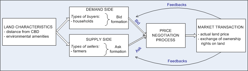
Figure 1. Conceptual scheme of the land market

3.3

The land market in ALMA is represented as a two-side matching market. Our goal in this paper is to present a somewhat simplified version of the standard monocentric urban model (Alonso 1964). Therefore, each spatial good is characterized by distance to the CBD, and by uniformly distributed environmental amenities. Buyers form their bid prices for land depending on the distance to the CBD, their preferences for commuting, budget constraints, and potentially market conditions. Sellers form their ask prices based on a fixed opportunity cost, and potentially market conditions. When two trading partners are able to agree upon transaction of a spatial good, the land is transferred to the new user. Thus, ALMA-v1.0 produces urban land patterns and land prices (land rent gradients) as a result of market allocation of land between competitive users. The environment and main entities of ALMA-v1.0 are shown in Figure 2.

3.4

The code of the ALMA model also provides the possibility a) to represent heterogeneous environmental amenities and disamenities, b) to account for spatial externalities that serve as feedbacks from the changed spatial structure of a neighborhood when a spatial good changes its owner, and c) to endow agents with heterogeneous preferences for environmental amenities and proximity to the CBD (Filatova, Parker et al. 2007; Filatova, van der Veen et al. 2007; Filatova and van der Veen 2007). For the purposes of this paper this capacity is not utilized.

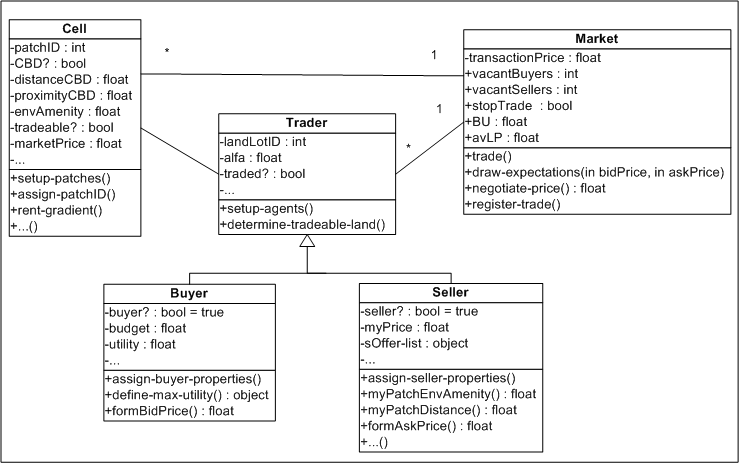
Figure 2. UML class diagram of the ALMA-v1.0 metamodel[2]

3.5

We proceed with the description of ALMA-v1.0 following the MR.POTATOHEAD framework (Parker, Brown et al. 2008). First, the spatial environment will be described in detail, then we will explain the behavior of economic agents. We conclude with a description of the land exchange mechanism.

The spatial environment

3.6

Space is an essential component of any land market. ALMA-v1.0 has an explicit spatial representation of model dynamics (i.e., the location of the CBD and relative transportation costs affect model dynamics and the spatial pattern of land rents resulting from market trades). Space is represented by a grid of equal cells, each of which can be owned by one economic agent. Each cell can be viewed as a separate spatial good, e.g. property unit, characterized by several parameters (see Figure 2). In ALMA-v1.0 each cell has two characteristics: distance from the CBD and level of green amenities. In principle, cells can be parameterized with more characteristics if needed.

3.7

The position of the city center (CBD) is exogenous and is in the center of the 2D lattice, i.e. it is a point with coordinates (0;0) in a Cartesian coordinate system. A distance of each cell (D) is measured as a Pythagorean distance from the center of coordinates. We also estimate relative proximity to the CBD (relative meaning that it is compared to the maximum distance in this city) as a measure inverse to distance (Equation (1)). Here D_max is a distance from the CBD of the most remote cell in the simulated landscape, dependent on the extent of the landscape as set by the user. In this paper, we run the model on a 29×29 lattice, but the landscape extent may be extended as needed. Thus, relative proximity for distance D is given by:

(1)

Further, when agents estimate their utility for a certain property unit, they use a normalized value of proximity:

(2)

The standard monocentric model assumes that households choose a location in the city as a result of the tradeoff between land price and transport costs. Transport costs are assumed to be a linear function of distance: T(D)=tcu*D, where tcu are transport costs per unit of distance.

The demand side of the land market (acquires of land)

3.8

Buyers are households searching to buy a house/land lot. At model initialization, the number of buyers is defined by the user.

3.9

Budget: As we discussed earlier, in traditional urban economic models households search for a location to maximize their utility under their budget constraint. While transferring the equilibrium economic framework into an ABM market, we have to make a few assumptions, which arise when one attempts to transfer the traditional budget-constrained utility maximization framework to an agent-based model (Parker and Filatova 2008). In ALMA-v1.0, we first assume that the housing choice is separable —i.e. the buyer has already decided what portion of her income to spend on housing and non-housing goods. This assumption is consistent with traditional real estate markets, where in general about one third of household monthly income is spent on housing (i.e., the mortgage payment). Thus, we assume that household agents have already estimated their disposable budget for housing and transportation before they come to the land market. The budget constraint of a buyer is the disposable budget for housing ( Y_housing, i.e. "budget" attribute of buyers on Figure2) net of transport costs at a certain distance D:

(3)

Second, at this point of the model development it is assumed that each seller owns only one spatial good (i.e., one cell) and each buyer is interested only in buying one property unit. We leave for future work the question of the amount of floor space/land lot area demanded.

3.10

Utility: Thus, the task of a house buyer is reduced to a)a choice of the housing good that gives maximum utility under her budget constraint, and b)estimation of her WTP. Households' utility depends on the qualitative characteristics of a spatial good, which depend on its location, and is assumed to have a Cobb-Douglass functional form (Equation (4)). Here A is the uniformly distributed amenity, P is normalized relative proximity estimated according to Equation (2), α and β are preferences for green amenities and proximity respectively, and α + β =1. For the model experiments presented here, we assume that α > 0.5. As in the original Alonso (1964) model, distance is included directly in the utility function because it represents not only the travel costs but also the disutility of commuting time to the CBD, which decreases the overall utility of a remote location.

(4)

3.11

Bid price: Given her utility function and budget constraint, a buyer chooses which property to bid on by sampling N spatial goods, offered for sale in the current market, that are affordable given her budget constraint. She then calculates the utility of each spatial good, and chooses to bid on the one for which her utility is the highest (see Figure 3).

3.12

In standard economic theory, the relationship between individual WTP and qualitative characteristics of housing is given by the demand curve of a household^[3]. WTP is assumed to be a function of utility, individual income and prices of all other goods (Varian 1992). We propose to describe these dependencies with the help of the following function^[4]:

(5)

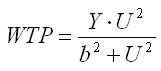
Here, Y and U are calculated according to Equations (3) and (4) respectively, and b is a constant. Function (5) is monotonically increasing approaching Y as U → ∞, meaning that individual WTP increases with utility but does not exceed her budget. The value of parameter b controls the steepness of the function. As b → ∞ the function (5) becomes flatter, and at U = b, WTP = Y/2, reaching half of its possible value. We can think of b as a proxy of the affordability of all other goods to reflect their relative influence on the WTP for housing. As shown in Appendix A, the WTP function (5) exhibits the main qualitative properties of the neoclassical demand function.

3.13

We differentiate between WTP and a final bid price of a buyer, and between WTA and a final ask price of a seller (Parker and Filatova 2008). In the bilateral trading and negotiation of a land market, buyers try to maximize their gains from trade (the difference between their WTP and their bid price), as do sellers. Therefore, they will set a bid price below their initial WTP, but they will attempt to keep their bid above the WTA of a seller. However, agents are likely to perceive the negotiating power of their trading partners depending on whether it is a sellers' or a buyers' market. In a sellers' market, demand exceeds supply, and sellers obtain more market power to influence the final transaction price, while buyers have to compete more intensely to be able to obtain needed goods. In this case the buyer's bid price is likely to grow in order to increase the chance that they will outcompete other buyers and obtain the desired good. In contrast, in a buyers' market when supply exceeds demand, buyers have more market power to influence prices, and sellers must reduce their relative ask prices in order to be able to sell. We believe that these market feedbacks, at least partly, explain cyclical dynamics in the housing market. Price adjustments depending on demand or supply excess in financial ABM markets are commonly modeled (LeBaron 2006). We translate this conceptual framework into housing market dynamics using the following strategy to adjust bid and ask prices depending on the relative market power of buyers and sellers. In ALMA-v1.0 a bid price of a buyer is estimated as follows:

(6)

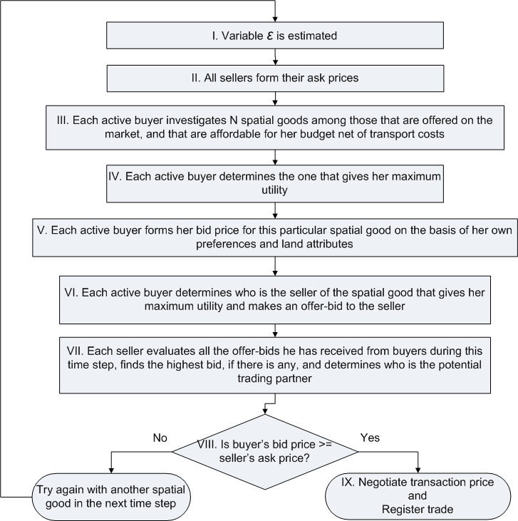
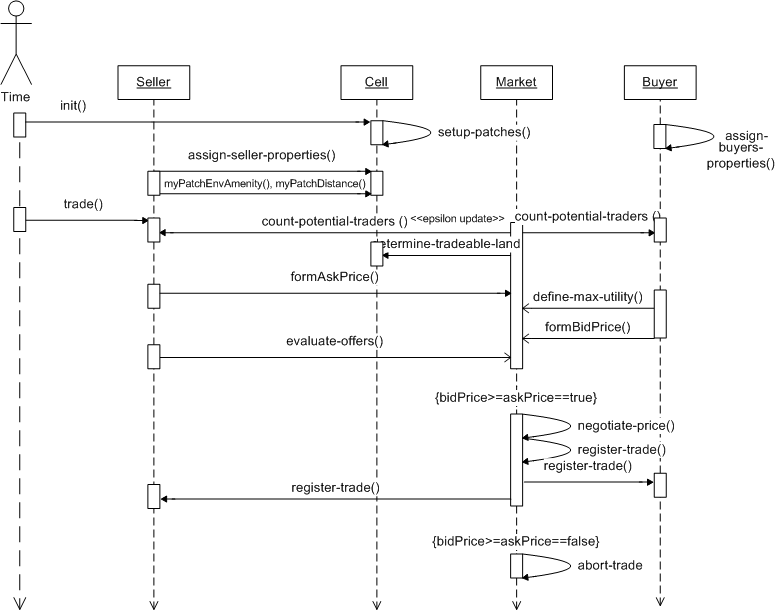
where NB is the number of buyers and NS is the number of sellers. Both variables indirectly depend on land prices and the number of successful transactions in the previous time step, since if prices are beneficial for both buyers and sellers, they participate in successful trades and leave the land market. If an imbalance of buyers and sellers remains, bid or ask prices will adjust to correct the imbalance. At the beginning of each time step, the variable ε is updated and pricing behavior changes (See Figure 3).

3.14

Properties of ε: If the number of buyers exceeds the number of sellers (i.e., it is sellers' market) then ε > 0, and P_bid increases, as buyers compete to be able to buy the spatial good they want. Correspondingly, if ε < 0, then sellers compete for the buyers, and buyers in their turn are willing to pay relatively less and sellers may accept lower bids.

3.15

The relative change in bid price will also depend on the total number of buyers and sellers in the marketplace, reflecting the logic that a small number of buyers and/or sellers will increase the market power of the participants. If total number of traders is small, , and the absolute value of . In this case, a change in the relative number of buyers and sellers will cause a relatively large change in bid prices, leading to relatively large change in transaction prices. This situation can be viewed as an oligopoly (a market dominated by a few suppliers of a good) or an oligopsony (a market dominated by a few buyers), where each dominant agent can influence prices significantly. If the total number of traders is large, , and . This situation can be viewed as the case of monopolistic competition, where there are many buyers with heterogeneous preferences and many sellers who offer heterogeneous goods. In this case, a change in the relative number of buyers and sellers will lead to relatively small changes in bid prices and transaction prices. One individual has little influence on land prices as possibilities for substitution are high, and the average market price for land changes slowly with time. Thus, in summary, the numerator of ε determines whether the final bid price will decrease or increase, and the denominator defines the magnitude of the change.

3.16

Bounded rationality: In our model, as in the neoclassical model, agents are assumed to maximize utility by choosing the optimal location under the budget constraint. However, there are two important distinctions from the neoclassical utility-maximization problem. Neither buyers nor sellers account for their future benefits, and in that sense they are myopic, as they do not calculate the optimal time to enter the market. Moreover, economic agents are not fully-informed. The search for the optimal transaction in any market is costly. This search involves information, time and monetary costs, meaning that a global optimum is not likely to be located in real-world housing markets. As well, humans have limited computational abilities: even if they might have full information about all houses on the market, it is not a trivial task to find a maximum (of utility) on this n-dimensional space (where n is the number of attributes of a spatial good). In other words, replicating the limitations imposed on real-world traders by this computational complexity we make economic agents in the ALMA model boundedly rational.^[5]

The supply side of the land market (suppliers of land)

3.17

Sellers represent owners of agricultural land. At model initialization, the user defines the number of sellers NS. The model experiments presented in this paper have a fixed number of sellers equal to the number of cells in the initial landscape. Each seller owns one land lot. Consistent with the monocentric urban model, in ALMA-v1.0, the supply side is assumed to be willing to give up its land at the fixed price of agricultural land, which is the same everywhere in the city ( P_ag is equal 200 in our experiments). However, sellers try to capture economic surplus from converting land to urban use. Therefore, we assume that they set their WTA 25% higher than their reservation price but still the same everywhere in the city ( WTA =250).

3.18

As widely discussed in our earlier paper (Parker and Filatova 2008), in general the ask price is expected to differ from a seller's WTA. When sellers form their ask price, they may account for the market situation:

(7)

The variable ε is estimated as in Equation 6. In the case of a buyer's market, when sellers decrease their ask price ( P_ask), we impose a condition that the ask price cannot go below agricultural reservation price ( P_ag).

Price negotiation and market transactions (land exchange mechanism)

3.19

Land exchange rules: The algorithm that artificial traders follow is presented in Figure 3. Location choice and the price for the desirable site are determined jointly. Thus, the decision of an agent to buy a house is divided into two stages: a) finding a spatial good that maximizes her utility (step III. and IV., Figure 3) and b) determining transaction land price (steps V.- IX.). The seller gathers all bids for his property offered during the current time step and selects the highest of these bids. Nevertheless, the market transaction will only take place if the terms of trade are favorable to both the buyer and the seller (see box VIII.). If, however, the buyer's bid price is higher than the seller's ask price, meaning that gains from trade are potentially positive for both traders, there are several possible ways to determine the actual transaction price for the spatial good. Price negotiation mechanisms in existing market ABMs vary from simple arithmetic or geometric average of bid and ask prices (Berger 2001) to sophisticated algorithms, such as auctions (Miyake 2003; Polhill, Parker et al.2008). For simplicity at this stage of the ALMA model, the price negotiation procedure (step IX.) is implemented as a calculation of the arithmetic average of the seller's price and the highest offer-bid of a buyer. A successful trade is registered by ALMA-v.1.0 (step IX.), both buyer and seller update their status (the seller will not sell in the next period, the buyer will not search for a land lot to buy, and they will not be counted in the estimation of NB and NS in Equation 6), the ownership rights on the spatial good are transferred from seller to buyer, and the transaction price is registered as the actual price for this specific land lot. Both the exchange of land and recording of the market transaction are fulfilled by a "Market" agent (Figure 4) and are saved in a *. csv (comma separated values) file. The numbers of buyers and sellers remaining in the market after the transaction will influence the determination of bid and ask prices in the next time step via the variable ε (see Equations (6) and (7)). The model stops running when no more transactions occur, i.e. all the submitted bids are lower than ask prices^[6]. Implicitly we assume that households (i.e., buyers) not settling in this city will search for a location in another city and leave the simulation environment, as in the open city model (Straszheim 1975; Anas, Arnott et al. 1998).

Figure 3. Conceptual algorithm of trade

3.20

Event sequencing mechanisms: In any given time step, Netlogo activates agents in a random, but fixed, sequence. In the first time step of any model run, a preset number of buyers and sellers are initialized. Below, we present experiments with and without activation of ε (realized via assigning "Pure WTP/WTA" or "Market-oriented" pricing behavior to traders). In the "Pure WTP/WTA" case, all buyers are activated in each time step. In the "Market-oriented" case, all buyers may not be activated in each time step, but instead will become active in the market at some user-defined rate. Epsilon is calculated using all the initialized buyers and sellers who have not yet successfully traded, not only those who are active in trading in a given round. The number of buyers who are active in the market in each time step (buyers from previous time periods who have not successfully purchased properties plus newly activated buyers) affects the speed at which ε is updated (see Experiments 3-6). The lower the number of buyers active in the land market during the time step, the more often ε is updated. Buyers and sellers who have not completed a successful transaction remain active in the next time period. The model continues to run until no more transactions occur.

3.21

The sequence of events in ALMA-v1.0 is presented in Figure 4 below. The scheme is quite straightforward and all the components were discussed above.

Figure 4. UML time sequence diagram

3.22

Innovations of ALMA : The ALMA model allows us to study the division of gains from trade in the land market, since there is a differentiation between ask price and WTA, and bid price and WTP. A consumer's (producer) surplus is the amount she (he) benefits from being able to buy (sell) a good at a price below her WTP (above his WTA). In the traditional equilibrium framework, the price at which everyone buys (sells) is assumed to be the price determined at equilibrium by some hypothetical auctioneer, and this price is used to calculate consumer and producer surplus. In our ABM market, there is no one unique price for everyone in the market; rather, there is a set of individual transaction prices determined by each set of trading partners separately. Consumer (and producer) surplus is calculated by comparing WTP (WTA) with the individual transaction price (not an equilibrium one). The total economic surplus is the sum of consumer and producer surplus. In contrast to the approach taken to calculating consumer and producer surplus in the SLUDGE model (Parker and Meretsky 2004), this approach allows us to examine how consumer and producer surplus, influenced by relative market power, change as market conditions change.

Simulation Experiments

4.1

We performed several experiments with the ALMA model. The model produces spatially explicit rent gradients (i.e., land prices at different distances from the city center) and land patterns. We are mainly interested in how changes in buyers' and sellers' characteristics, environment, and trading strategies affect economic indicators and the spatial morphology of the city.

Macro-scale outcome measures

4.2

In addition to graphical representations, we also present a set of metrics to analyze micro and macro economic and spatial outcomes, including:

• Individual utility: the average individual satisfaction from the consumption of a good of a certain quality (characterized by certain parameters such as distance or environmental amenity), estimated as an average of individual utilities from equation (3);
• Aggregated utility: the total utility of all individuals settled in the city, estimated as the sum of the utilities of urban inhabitants (excluding agricultural users). This metric is often used as a measure of social welfare;
• Buyer's bid price: the average bid price for urban land, estimated as an average of individual bid prices (Equation (6)). This metric allows us to analyze how bid prices change depending on pricing strategy;
• Urban land price: the average transaction price in the city. The transaction price for the bilateral trade is an arithmetic average of a bid and an ask price. We are interested in how the transaction price changes depending on whether buyers or sellers account for the market situation;
• Average surplus (for both buyers and sellers): the average amount that buyers (sellers) benefit by buying (selling) a good for a price that is lower (higher) than their WTP (WTA). It is calculated as an average difference between the transaction price and buyer's WTP (seller's WTA). Comparison of the relative proportion of surplus captured by buyers and sellers allows us to analyze how the division of gains from trade changes depending on the market situation. Total economic surplus (i.e., the sum of a buyer's and a seller's surpluses) is also often used as a measure of social welfare;
• Total property value: the sum of urban land prices in the city. Total property value is important for policy analysis, particularly with respect to property taxes rates and receipts, funding of public goods from property taxes or estimation of the damage from extreme events such as flooding;
• City size: the number of urban inhabitants (excluding agricultural users). City size is a typical characteristic of urban spatial structure often analyzed in urban economics (Strazsheim 1987);
• Distance at which city border stops: the distance from the CBD of the most remote urban cell, or urban extent. Urban extent is also a typical characteristic of urban spatial structure used in urban economics. In the experiments presented here (with no open-space amenities), it will be closely correlated with city size;
• Estimated land rent gradient: an equation that quantitatively characterizes the realized transaction price at a given distance from the city center, estimated using linear regression analysis. The land gradient is another typical characteristic of urban spatial structure that is analyzed both theoretically and empirically in both urban economics and geography (Straszheim 1975; Anas, Arnott et al. 1998).

4.3

All the model experiments presented in this paper were performed on a 29x29 cell landscape. Each experiment was performed 30 times to check the robustness of the simulated results against random effects using a t-test. The ALMA parameters that remain unchanged for all model experiments are listed in Table 1; those that were varied between the 6 experiments are listed in Table 3. A brief summary of each experiment is presented in Table 2. The setup and objective of each experiment are discussed below. Tables 4 and 5 compare the experiments' outcomes in terms of macro and micro economic and spatial measures. Metrics for each experiment in Tables 4 and 5 are average estimates of 30 runs. Outcomes of each on the 30 runs in one parameter space do not change qualitatively. In particular, the standard deviation of total property values between the 30 runs in Exp 1-2 is equal to 0 and the standard deviation of total property values between the 30 runs of Exp 3-6 varies from 0.01%-0.04%.

Table 1: Values of parameters unchanged in the simulation experiments
Symbol	Y	A	b	N of cells	P<sub>	WTA
Meaning	Individual budget	Level of green amenities	A constant in (5)	Number of spatial goods in a city	Reservation price for agricultural land	WTA for agricultural land without consideration of the market situation
Value	800	1	70	841	200	250

Table 2: Description of the performed experiments
Experiment #	Tested hypothesis
Exp1	An agent-based ALMA model with distributed price determination mechanisms reproduces the conventional analytical model behavior given similar assumptions, i.e. structural validation holds.
Exp2	Increased tolerance for commuting among buyers (changes in preferences for distance - _) causes urban expansion.
Exp3	In the case of a "sellers' market" gains from trade will not be divided equally and the city will expand, assuming that buyers adapt their bid prices based on the market situation.
Exp4	The more often buyers are faced with information about market conditions, the more likely they are to "panic" and to offer higher bids.
Exp5	In the case of a "buyers' market" gains from trade will mostly be captured by buyers, assuming that sellers adapt their ask prices based on the market situation.
Exp6	The more often sellers are faced with information about market conditions, the more likely they are to "panic" and to offer lower ask prices.

Table 3: Values of parameters changed in the simulation experiments
Symbol	Meaning	Exp1	Exp2	Exp3	Exp4	Exp5	Exp6
NB	number of buyers	841	841	925	925	757	757
NS	number of sellers	841	841	841	841	841	841
MB	market behavior	Pure WTP/WTA	Pure WTP/WTA	Buyers:Market oriented	Buyers:Market oriented	Sellers:Market oriented	Sellers:Market oriented
Betta	preference for proximity to the CBD	0.85	0.7	0.85	0.85	0.85	0.85
N-buyers in trade	number of buyers activated each trade period, i.e. the speed of epsilon (ε) updating	all	all	all	5	all	5
TCU	transport costs per unit of distance	1	1	1	1	1	1

Table 4: Economic and spatial metric outcomes of the ALMA experiments
Parameter	Exp1	Exp2	Exp3	Exp4	Exp5	Exp6
Individual utility: Mean	65.48	66.61	63.51	62.19
St.dev	12.56	12.6	13.29	13.8
Aggregate utility	30448.82	38431.14	32836.11	34391.27
Buyers' bid price: Mean	363.72	369.97	371.99	374.82	342.24	342.26
St.dev	73.92	73.53	80.21	80.53	83.99	83.98
Urban land price: Mean	306.86	309.98	311	312.41	286.35	285
St.dev	36.96	36.77	40.11	40.27	44.99	45.17
Average surplus %:Buyers'	50%	50%	39.58%	38.19%	60.59%	62.06%
Sellers'	50%	50%	60.42%	61.81%	39.41%	37.94%
Total property value	142690.2	178860.2	160785.6	161494.5	158350.8	157587.1
City size (urban population)	465	577	517	553
Distance at which city border stops	12.08	13.45	12.81	13.15

Table 5: Linear regression estimation results of the ALMA model generated data (the transaction price is a dependent variable)
Parameter	Exp1	Exp2	Exp3	Exp4	Exp5	Exp6
R2:	0.9905	0.9858	0.9913	0.9899	0.982	0.982
Intercept: estimate	410.76	413.2	423.9	425.68	412.39	411.57
St error	0.09	0.1	0.09	0.1	0.14	0.14
t-Value	4498.96	4136.46	4710.81	4360.21	2936.39	2917.12
Distance to CBD: estimate	-12.81	-11.43	-13.2	-13.25	-14.25	-14.31
(slope) St error	0.01	0.01	0.01	0.01	0.01	0.02
t-Value	-1207.17	-1096.03	-1330.84	-1230.62	-951.96	-951.55

Replication and sensitivity analysis of Alonso model

4.4

In this set of experiments we explore how the dynamic land market model behaves. We mainly focus on the tasks raised by research question 1 in section 2 above.

4.5

Experiment 1: The purpose of this paper is first to replicate the benchmark case of the analytical Alonso model (i.e. perform structural validation), and then, moving from this comparison baseline, to demonstrate the valued added from the agent-based approach. Summarizing the baseline assumptions of ALMA-v1.0, buyer agents have homogeneous preferences for proximity to the CBD and bid their willingness to pay, which is based on their preferences for proximity, their housing budget, and the transport cost to their preferred cell. Sellers, i.e. owners of agricultural land, each offer land at the same fixed price. Neither buyers nor sellers account for the market situation (i.e., for epsilon). The main difference between this simulation experiment and the analytical model is that the centralized land price determination mechanism is replaced by a series of spatially distributed bilateral trades. However, since agents are homogeneous and no market situation is accounted for while bidding, our model reproduces the standard Alonso pattern of land rents predicted by the analytical equilibrium, meaning that transaction prices are equal for all cells at an equal distance from the CBD. The results from the replication of the Alonso model are presented in column "Exp1" of Table 4. The spatial form of the city and urban land rent gradient are presented in Figures 5.a and 5.b respectively.

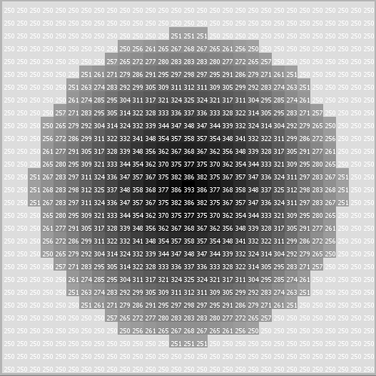
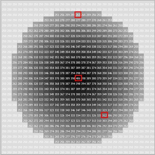
Figure 5.a. Exp1, Replication of the Alonso model: a) Spatial form of a city

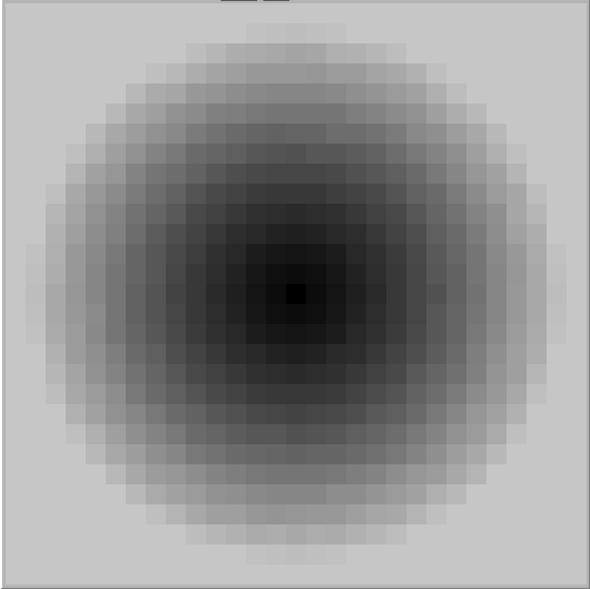
Figure 5.b. Exp1, Replication of the Alonso model: b) Land rent gradient

Figure 5.c. Exp1, Replication of the Alonso model

4.6

The green area in Figure 5.a represents agriculture and the black is urban area. The intensity of grey color in Figure 5.b symbolizes the value of land: the darker the color, the higher the land price. As in the benchmark case of a theoretical monocentric urban model, land prices are higher closer to the CBD, and the land rent gradient is decreasing with distance. The urban land price is equal for cells that are equidistant from the CBD (as seen in Figure 5.c). The city expansion stops at the location where bid price of a buyer falls below the agricultural rent (P_ask=250). The lightest-grey area in Figure 5.b shows the beginning of the agriculture area (urban-rural fringe) and symbolizes the city border. Note that not all of the buyers in the model ultimately purchase properties (only 465 of the 841 buyers engage in transactions). The parameter settings for Exp1, then, replicate an open city model, where buyers are assumed to have the opportunity to purchase a property in another location, if their WTP for available properties in this region is below the WTA of the current landowners. We did other experiments with the ALMA model, such as changes in income or increase in transportation costs - traditional tests performed with analytical urban models. As in the base case described in Exp1, the ALMA model reproduces qualitative results of the conventional equilibrium model.

4.7

We estimated a functional representation of the rent gradient through a linear regression analysis of the model-generated data. We tried several functional forms including linear, log-log (both sides of the equation are in logarithms), semi-log (the dependent variable is in logarithm and the right hand side is in linear forms) and inverse semi-log form (the dependent variable is linear and the right hand side is in logarithms). The R² values from these four model specifications are 0.9905, 0.9764, 0.8599 and 0.8236 respectively. The results of the linear regression model, which showed the best fit, are presented in Table 5 and in Figure 7. The graphic of the regression line together with the transaction data from Exp1 is presented in Figure 7 (the blue line and scatter points).

4.8

Experiment 2: We now wish to conduct a sensitivity analysis of how buyer preferences influence our proposed metrics (Table 4) and change the slope of a rent gradient (Table 5 and Figure 7). The setup Exp2 is identical to Exp1 (see Table 3), but with a lower preference for proximity to the CBD for buyer agents (particularly _ = 0.7 instead of 0.85), which can also be interpreted as a higher tolerance for commuting. The first difference in results from Exp1 manifests itself in the spatial morphology of the city, as seen from comparison of Figures 6.a and 5a. The city border has expanded (shifted from 12.08 spatial units in Exp1 to 13.45 in Exp2), and the urban population has increased (from 465 to 577) as can be seen from Table 4. The land rent gradient (Table 5) is decreasing with distance as in Exp1. However, the prices of cells at the same distance from the CBD in Exp1 and Exp2 differ due to the difference in preferences (compare land prices in Figures 5.c and 6.c). The price of the most central cell is the same (due to the normalization of distance in the utility function), but the prices of more remote cells are higher in Figure 6.c than in Figure 5.c—with a higher tolerance for commuting, the buyers' willingness to pay for remote cells has increased. Moreover, the price difference between two experiments increases with the distance from the CBD which is consistent with the concavity of the utility function with respect to proximity. (See Figure 6 as well.) This result demonstrates the advantage of including a preference for proximity in the utility function, as was the case with the original Alonso model, rather than simply using transportation costs as a proxy for commuting disutility. Average land price is higher in Exp2 than in Exp1 (explained by the higher rent gradient), and total property value in the city is also higher (explained by the greater urban expansion) (see Table 4). The result is statistically significant at the 99% confidence level as confirmed by the t-test (see Appendix B). Since buyers have a higher tolerance for commuting they are more willing to buy land in the remote areas. Thus, buyers in Exp2 are willing to pay more for housing at a given distance from the CBD than are buyers in Exp1 at the same location, and they also can offer bids higher than sellers' ask prices on properties at higher distances from the CBD. The result is higher average bid prices in Exp2 (the average bid price is 363.72 and 369.97 in Exp1 and Exp2, respectively).

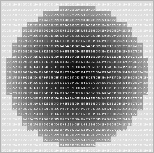
Figure 6.a. Exp2, Preferences for proximity are lower than in Exp1 in Figure 5: a) Spatial form of a city

Figure 6.b. Exp2, Preferences for proximity are lower than in Exp1 in Figure 5: b) Land rent gradient

Figure 6.c. Exp2, Preferences for proximity are lower than in Exp1: Lad rents

4.9

To compare the land rent gradients between Exp1 and Exp2, we again estimated the land rent gradient for the computer-generated data from Exp2. The linear regression model again showed the best fit in comparison to other functional forms (the R² is 0.9858 in comparison to 0.9696, 0.8430 and 0.8061 of log-log, semi-log and inverse semi-log forms respectively). Consistent with the results described above, the regression coefficients in Table 5 for Exp1 and Exp2 differ. A visual comparison of a regression analysis of the computer generated data (Table 5) from Exp1 and Exp2 is presented in Figure 7. The supply curve of agricultural agents is a constant line (equal to 250 in our settings) parallel to the axes OX. The point at which the regression line and the line y = 250 cross shows the distance at which city expansion stops, i.e. at which the transaction price is lower than sellers' ask price. Both estimated rent gradients are downward slopping, meaning that land price is deceasing with distance from the CBD, as in the Alonso bid rent theory. However, as expected, the slope of the rent gradient (the regression coefficient for distance to the CBD) for Exp1 is higher in absolute value than the slope of the rent gradient from Exp2 (Table 5); i.e. the bid rent curve in Exp1 is steeper than in Exp2. The gap between the estimated rent gradients also increases with distance from the CBD, consistent with the explanation presented above--at higher distances from the CBD the more commuting-tolerant buyers will always bid higher than the people with strong preferences for proximity to the CBD.

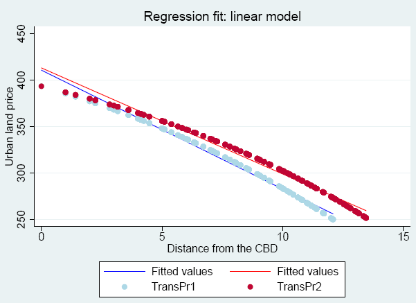
Figure 7[7]. Land rent gradients for Exp1 and Exp2, linear regression fit of the computer generated data TransPr1(2)- actual land transaction prices from Exp1(Exp2 - lower preferences for proximity), Fitted value - estimated land rent gradient

Market-oriented buyers and sellers

4.10

In the previous experiments, we have run ALMA-v1.0 with traders who do not account for the relative power of buyers and sellers, i.e. for epsilon in Equations (6) and (7). Both household-buyers and agricultural sellers thus revealed their true WTP and WTA while submitting bids and asks to the market (see Figures 1 and 2). In the next few experiments, we implement another market behavior: instead of revealing their pure WTP/WTA, agents adjust their bids and asks depending on whether it is a sellers' or a buyers' market-in other words, they become market-oriented. In order to answer the second research question from section 2 above, we analyze macroscopic model outcomes from experiments that implement different pricing strategies at micro level. We increase or decrease the number of buyers in the land market to replicate buyers' or sellers' markets, activating ε in Equation (6) when the number of buyers exceeds the number of sellers, and activating ε in Equation (7) when the number of sellers exceeds the number of buyers. Code verification using the parameter settings for Exp1, but de-activating ε (so that agents submit bids and asks without accounting for the market power of each other) confirmed that unequal numbers of buyers and sellers at the land market did not affect outcomes for homogeneous agents, as expected.

4.11

Experiment 3: In this experiment we investigate how the morphology of the city and economic indicators will change if buyers change their bidding strategy in a "sellers' market" environment. We assume that while forming their bid price, buyers account for the market situation (i.e., account whether it is a buyers' or a sellers' market). We run ALMA-v1.0 with a higher number of buyers (10% more than sellers; see Table 3 for parameter settings). In this case, buyers realize that sellers have relative market power and that buyers have to compete for the spatial good, since there are more buyers willing to buy the good than there are goods on the market. Per Equation (6), they therefore increase their bid price above their initial willingness-to-pay in response (but still do need exceed their budget constraint). Agricultural sellers set their ask price at the price of agricultural land, i.e. equal to 250 as in previous experiments. The land rent gradient and spatial form of the city are shown in Figure 8. The simulated land rent gradient is reported in Table 5 and illustrated in black in Figure 10.

4.12

Over the time steps of the model run, buyers incrementally raise their bid prices and are willing to buy land further from the CBD even if they originally (in Exp1) would value it less then the P_ask. This temporal increase in the bid price can be viewed as an emergent model outcome, since it is the result of interactions between bidding agents. While the behavioral rule that bid prices will depend on buyer/seller ratios operates at an individual level, the implementation of this behavioral rule depends on the previous decisions of other agents (on the global state of the system). The average bid price (not to be confused with the final transaction price) has increased by 8.27 monetary units in comparison to the average bid price in Exp1 (see Table 4). The result is statistically significant at the 99% confidence level as confirmed by the t-test (see Appendix B). As a result of sellers' market power and buyers' competition, there is a significant change in the relative proportion of buyers' and sellers' surplus. In the case when buyers bid only on the basis of their utility (Exp1-Exp2), the proportions of surplus captured by buyers and sellers are equal. However, when sellers have more market power, they capture a higher proportion of gains from trade (60.42% vs. 39.58%), making themselves better off.

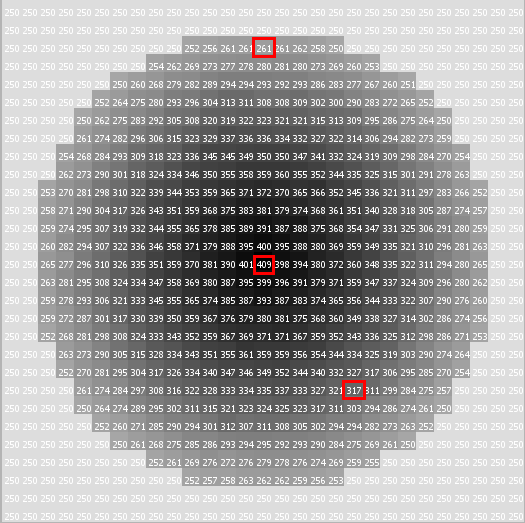
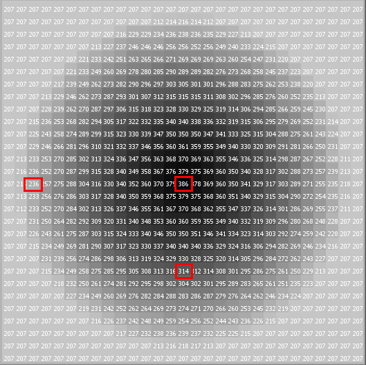
Figure 8.a. Exp3, Buyers' competition in a sellers' market: a) Spatial form of a city

Figure 8.b. Exp3, Buyers' competition in a sellers' market: b) Land rent gradient

4.13

In comparison with the outcome of Exp1, the city has expanded (compare Figures 5.a and 8.a). The city border has shifted from 12.08 spatial units to 12.81 in Exp1 and Exp3 respectively. The urban population has increased by 11.2%. The total value of the property in the city increased as well. The land rent gradient still follows the Alonso predictions, i.e. the rent decreases with the distance. However, the structure of the land rent gradient differs from Exp1; prices for land at the same distance from the CBD are not always equal, since buyers bid for the parcels at different time steps, each having a different market structure (different value of ε). Thus, if equilibrium in the land market is not achieved in one shot but is rather distributed (prices are determined in the bilateral trades in different moments in time), and if market participants respond to the relative market power of other participants, then prices for spatial goods with the same characteristics might not be homogeneous, even with homogeneous traders. This result differs from that of the traditional equilibrium-based theoretical model that assumes a centralized price determination mechanism such as a Walrasian auctioneer, which will predict that prices for a good of equal quality consumed by homogeneous economic agents will be the same. Sensitivity analysis (not presented here) demonstrated also that the larger the gap between the number of buyers and sellers in the market the larger the deviation of land prices in Exp3 (Figure 9.b) from Figure 5.c.

4.14

Experiment 4: Now we would like to show how the speed of ε updating (from Equation (6)) influences the model outcome. Our hypothesis is that the frequency with which agents received updated information concerning the market situation will affect the evolution of prices. The setup for this experiment is basically the same as in Exp3 except for changes in the buyer activation regime. In Exp3, all the buyers initialized in the model can participate in the market (see section 3.4 for discussion) in the first time step of the model. The value of ε is updated once per time step (see Figures 3 and 4), using the total number of buyers and sellers participating in a market (the original number of each, minus the number of each who have successfully completed a transaction in the last time step). In Exp4, we allow fewer buyers to participate in market transactions in each time step. This means that the variable ε will be updated more frequently. In other words, buyers will have access to more accurate information regarding excess demand. More significantly, buyers have more frequent opportunities to update their bids to reflect new market conditions. (Note, however, that the number of buyers who are searching for properties (NB) is different than the number of buyers activated in each time step.) This situation could be viewed as that of a seasonal market, where some buyer agents enter earlier than others, and later buyers form bids based in part on their perception of current market conditions. Essentially, market prices are path dependent in the market-oriented pricing situation-the bid in a particular time period depends on the market situation in the previous time period. We run Exp4 with only 5 buyers activated per time step. The results of this experiment run are presented in column Exp4 of Table 4.

4.15

The spatial form and spatial metrics of the city stay exactly the same as in Exp3 (see Figure 8.a and Table 4 column for Exp3), as does average individual utility in the city. (Intuitively, utility is separate from bid price: having paid more for the property, the buyer still only receives the same level of utility.) The differences between the experiments are manifested in land prices. Land prices again are decreasing with distance to the CBD but even less gradually than in Exp1and Exp3. Figures 9.a and 9.b show land prices as the outcome of Exp3 and Exp4 respectively. All the parameters stay the same in these two experiments except for the speed of information provision to the buyers. As a result, buyers in Exp4 were willing to bid higher prices for the same houses as in Exp3. For example the most central land lot in Figure 9.b (from Exp4) was purchased for 409 monetary units in Exp4 in contrast to 406 in Figure 9.a (from Exp3). The price for almost every cell in Figure 9.b is higher than in Figure 9.a. As a result, the aggregate economic measures in Table 4, such as average bid price and urban transaction land price, are higher in Exp4 than in Exp3. The result is statistically significant at the 99% confidence level as confirmed by the t-test (see Appendix B). Most important, the division of gains from trade has changed: now sellers capture even more of the total economic surplus from the transaction than in Exp3.

Figure 9.a. Influence of the speed of ε updating on the land prices at a sellers' market: a) Land prices, Exp3

Figure 9.b. Influence of the speed of ε updating on the land prices at a sellers' market: b) Land prices, Exp4

4.17

Figure 10 shows land rent gradients estimated using the simulated data from Exp4 (Estimates in Table 5). The red dots and red line represent the transaction prices and estimated land rent gradient, respectively. We compare the estimated land rent gradient to those from Exp3 (the black line) and from Exp1 (the blue line). Both land rent gradients from Exp3 and Exp4 are much higher than the land rent gradient from Exp1, meaning that buyers bid higher at all distances from the CBD in Exp3 and Exp4. At the same time, we can see that the black line is a bit below the red line; i.e. buyers from Exp4 would outbid buyers from Exp3. The only reason for this is the increased speed of information about the market situation provided to buyers at the moment of their bid formation, and the corresponding increased speed of updating of bids.

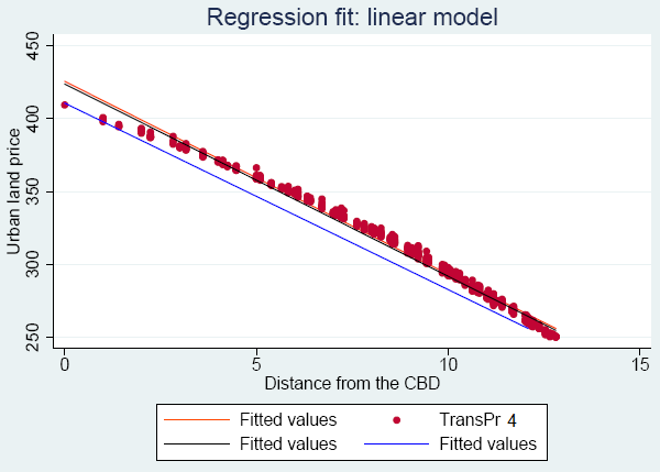
Figure 10[8]. Land rent gradients for Exp1, Exp3 and Exp4, linear regression fit of the computer generated data TransPr4- actual land transaction prices from Exp4, Fitted value - estimated land rent gradient: blue - for Exp1, black - for Exp3, red - for Exp4

4.18

Interestingly, one of the conclusions from this experiment might be that if there is a sellers' market and information about this fact is provided more often to the buyers (e.g. via newspapers or by real estate agents) then buyers will increase their bids for the same type of house, raising housing prices in a kind of "artificial panic". So, simply news of a high demand excess can create the effect of a housing bubble, causing prices to rise without an underlying economic rationale. This implies a certain set of incentives for real estate agents. If they want to increase the final transaction price (and the share of it they capture as their fee) they might want to emphasize that there is a demand excess in a particular housing market. In early presentations of ALMA, we received many comments about the importance of real estate agents to the dynamics of bid and ask price formation. This updating mechanisms, and the conclusions that it implies, is a first step toward more formal exploration of their potential role in housing market dynamics.

4.19

Experiment 5: In the previous experiment, we assumed that the number of buyers was higher than the number of sellers. Here we investigate the opposite situation: there are more sellers than potential buyers. Thus, buyers have market power in this land market. Now sellers are competing, and in order to be able to sell their agricultural lots they adjust their ask price depending on the market situation (i.e., ε in (7); again note that ε is activated only on the seller side). The economic metrics are presented in Table 4 and the spatial form of the city as well as land rent gradient are shown in Figure 11. The estimated land rent gradient is illustrated in Figure 12 and reported in Table 5.

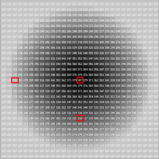
Figure 11.a. Exp5, Sellers' competition in buyers' market: a) Spatial form of a city

Figure 11.b. Exp5, Sellers' competition in buyers' market: b) Land rent gradient

4.20

In this market regime, sellers gradually decrease their ask price until it reaches agricultural land price. Since ask prices decrease, land at higher distances becomes more affordable for buyers. Thus, remote areas are converted into urban use, and city expands in comparison to Exp1 (compare Figures 11.a and 5.a). The city border expands as long as the buyers' highest bid is above sellers' reservation price. The average transaction price for land has decreased by 5.9% in comparison to Exp1 data (see Table 4). The decrease in land prices can also be seen in Figure 11.b, where the colors of land rent gradient became less intense in comparison to Figure 5.b. The result is statistically significant at the 99% confidence level as confirmed by the t-test (see Appendix B). Buyers have more market power in this situation and land prices are determined in their favor. As a result, average seller's surplus has decreased significantly in comparison to Exp1 (60.59% to buyers and 39.41% to sellers). As we can see from the estimated land rent gradients from Exp1 and Exp5 (Figure 12) the latter is lower than the former (see Table 5 for quantitative measures).

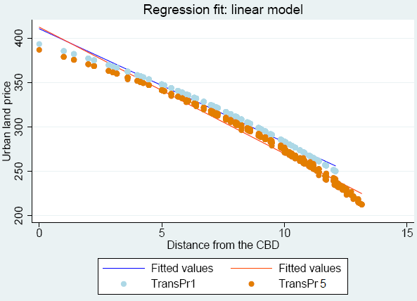
Figure 12[9]. Land rent gradients for Exp1 and Exp5, linear regression fit of the computer generated data TransPr5- actual land transaction prices from Exp5, Fitted value - estimated land rent gradient: blue - for Exp1, orange - for Exp5, dark green - for Exp6

4.21

Experiment 6: Finally, we ran ALMA with the same settings as in Exp5 but with a changed activation mode, replicating the logic of Exp4. Basically, we changed the number of buyers activated each time step in order to increase the speed of ε updating (from Equation (7)). We explore a buyers' market again but assuming that sellers more frequently update information about the market situation and integrate this information while forming their ask prices. The spatial form of the city stays exactly the same as in Exp5, but the land rent gradients change. Prices become even lower than in Exp5 (see Table 4 and Figures 13.a and 13.b for comparison). The estimated land gradient for Exp6 is a bit below the one from Exp5 (compare green and orange lines in Figure 12, see Table 5 for quantitative measures). The result is statistically significant at the 99% confidence level as confirmed by the t-test (see Appendix B). Thus, when sellers receive a consistent flow of information that it is a buyers' market and update frequently in response, they decrease their ask prices to attract potential buyers. Again, experiments with the speed of ε updating highlight the importance of the role of the role of information in the market and reinforce our interest in future exploration of the role of real estate agents, who serve as information providers for both sellers and buyers.

Figure 13.a. Influence of the speed of ε updating on the land prices at a buyers' market: a) Land prices, Exp5

Figure 13.b. Influence of the speed of ε updating on the land prices at a buyers' market: b) Land prices, Exp6

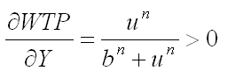
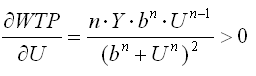
Discussions and Future Work

5.1

In this paper, we have presented an agent-based land market model that, in its simplest form, replicates the qualitative properties of the standard equilibrium-based monocentric urban market model. We have demonstrated that both micro-scale and macro-scale model behavior conform to the qualitative behaviors of the standard model. The WTP of buyer agents follows traditional rules, increasing with income, the relative prices of other goods, and the utility gained from the housing good, and decreasing with transportation costs. The model reproduces the standard result that when homogeneous traders operate in a homogeneous landscape, transaction prices (land rents) are the same at locations equidistant from the CBD, and land rents decline monotonically as distance from the CBD increases. The land rent gradient is estimated through regression analysis, using our generated transaction prices as the dependent variable, and distance as the independent variable. The extent of the urban area is determined by the location where the bid of the highest-value buyer is just equal to the willingness-to-accept of the seller (the opportunity cost of land in a non-urban use).

5.2

This replication exercise can be viewed as a sensitivity analysis or structural verification, ensuring that the model operates as intended, through comparison to an existing alternative theoretical model. We anticipate that the added value of the modeling effort will be seen as we move forward from this point. In, fact, it is the features of the model that relax the restrictive assumptions of traditional equilibrium models that will provide its utility. Moving beyond traditional models, our model separates the underlying valuation of buyers and sellers (their WTP and WTA) from their bid and ask prices, facilitating modeling of strategic pricing behavior, and analysis of the division of gains from trade under different market circumstances. The movement away from a pure optimization framework allows us to explore boundedly rational formation of bid and ask prices, as influenced by inductive updating of price expectations (see Parker and Filatova (2008) for more details). The ability to generate realized transaction data that can be used to estimate rent gradients through regression analysis allows us to more closely link our theoretical models to real-world data. Essentially, we have created a computational laboratory in which we have a full understanding of the agent-level and spatial factors that influence bid prices, ask prices, and realized transactions. This laboratory lets us explore the statistical predictions that emerge from these models, creating an opportunity for greater understanding of the potential processes that have generated the transaction data that we observe in the real world.

5.3

In this paper, we explore the implications of the model's ability to separate WTP (WTA) and bid price (ask price) formation for urban morphology and land prices. Starting from a baseline case where both buyers and sellers bid their true valuations, and gains from trade for successful transactions are evenly divided, we model bid and ask prices as depending on the relative market power of buyers and sellers. In this model, bid and ask prices adapt as market conditions change. We demonstrate that this process of price adaptation results in heterogeneous transaction prices over time for properties of the same quality (distance from the CBD in this simple case). It also results in conversion of properties that would not have been converted in the previous situation (more urban expansion). Finally, it results in a higher proportion of the gains from trade from transaction accruing to the market agents who have relative market power.

5.4

We then decrease the number of market participants in each time step (or, effectively, increase the speed at which participates update their bids). We show that this more frequent updating again increases prices for properties the same distance from the CBD. It also increases the proportion of gains from trade that accrue to the agents with relative market power. This result implies that more frequent provision of information to buyers and updating of bid prices leads to higher prices, creating an obvious incentive for agents in the market who benefit from higher prices to increase the intensity of provision of market information.

5.5

One interesting result of our analysis is that market-oriented pricing behavior on either the buyer or seller side leads to expansion of the urban area, although in one case land prices increase relative to the baseline (the sellers' market), and in the other they decrease. This result underlines the importance of modeling bid and ask price dynamics, rather than just assuming an equilibrium price that would result in the capture of equal gains from trade by both market participants. When either side has some relative market power, the result of the decreased bargaining power on the other side leads to more market transactions, and expansion of the city. Given the irreversible effects of conversion of rural land to urban uses, this finding is significant, although its full implications deserve more detailed consideration.

5.6

We plan several future directions for this model, including:

• Exploration of the effects of open-space amenities, including interactions between heterogeneous agent preferences and spatial heterogeneity;
• Modeling price expectation formation based on rates of change of prices (globally and within neighborhoods), as described in Parker and Filatova (2008);
• Modeling the decision of buyers and sellers to enter and leave the land market. The current model, ALMA-v1.0, is focused mainly on the exploration of land market dynamics and changes of economic and spatial macro outcomes depending on the changes in micro settings. There is an extensive literature on triggers for urban relocation (Clark and Van Lierop 1986; van der Vlist 2002). These motives could be included in the ALMA model;
• Modeling the optimal time to enter the land market and the dependence of agents' desire to sell or to buy a spatial good on agent-level factors (financial, social tension etc);
• Introduction of a "real estate" agent. This may be a natural way to model the process of learning about prices (Kirman and Vriend 2001; LeBaron 2001; Nicolaisen, Petrov et al. 2001; Tesfatsion 2006) in a land market context. It will also afford an opportunity to further explore the influence of information on the pricing strategies of traders.

Appendix A: Properties of the demand curve

A.1

In what follows, we would like to explore the properties of the buyer's willingness to pay (WTP, from Equation (5)) and to compare these properties to the properties of the traditional demand curve from microeconomics. This process serves two purposes. First, it allows us to gain a better understanding of the operation of our model at the micro (agent) level. Second, in keeping with our goal of replicating a standard economic analytical model, it ensures that the micro-level behavior of our model is consistent with the micro-level behavior assumed by the Alonso model. To derive some predictions of how our WTP function changes as its exogenous parameters change, we performed "comparative statics" analysis by estimating first-order derivatives of Equation (5) with respect to each parameter, while holding all others constant. The sign of the derivative describes the qualitative response of the WTP function to a change in the exogenous parameter. If negative, WTP falls; if positive, it increases.

1. Income effect : Microeconomic theory predicts that for normal goods an increase in income results in an increase in willingness to pay (demand).

   (8)

   This result is in line with microeconomic demand theory, in which an increase in income results in a positive change in the WTP, i.e. the demand curve shifts up. This fact means that if a buyer's purchasing power increases, her WTP also increases.

2. Changes in total utility : Although a buyer's level of utility is not observed in the real world, willingness to pay for the good is often used as an observed indicator to represent people's choices, for example in environmental economics. In theory, consumers are willing to pay more for those goods that bring them higher utility. Thus, a buyer's WTP for a spatial good that provides a higher level of utility should be higher than that for a spatial good that offers a lower level of utility. Certainly, this level of utility depends on other factors such as the level of the attributes given by the spatial good, and the buyer's preference weights for these attributes. We examine the effects of the preference weights below. However, to ensure the generality of the model, we first confirm that WTP is increasing with the utility provided by a particular good.

   (9)

   WTP increases as the utility of the good increases. An individual is willing to pay less for a spatial good that brings her lower utility and more for the one that brings her higher utility.

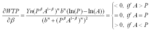
3. Preference for proximity effect : Again, in the real world, individual preferences, as well as utility itself, are unobserved. Nevertheless, intuition would predict that higher relative consumer preferences for an attribute of a good lead to a higher WTP for a good with relatively high levels of this attribute.

   (10)

   The result shows that WTP behaves differently depending on the characteristics of the spatial good. This result depends on the form of the Cobb-Douglas utility function (Equation (4)), which assumes a substitution effect between different characteristics of spatial quality (proximity to the CBD and environmental amenities). So, a buyer's WTP grows as preferences for proximity to the CBD increases if the proximity value of the good is higher than the amenity value of the good (P>A). In other words, as a buyer's preference for proximity increases, her willingness to pay for goods that provide more proximity than amenities increases, meaning that she will bid higher for a property closer to the CBD.

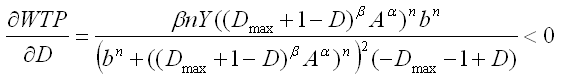
4. Effect of distance : One of the main properties of the demand for land function in the monocentric city model is that land price decreases as distance from the CBD increases. Alonso explained this result by the fact that both disutility of commuting and travel costs increase with distance from the CBD (Alonso 1964), p 71. Our WTP function should behave the same way, for the same reasons.

   (11)

   The derivative is negative because the expression (-Dmax-1+D) is always negative. This means that WTP decreases with distance to the CBD. Thus, it mimics the downward-sloping bid-rent function from the monocentric urban model.

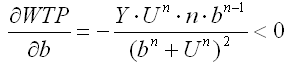
5. Effect of b : The willingness to pay for a spatial good depends among other factors on the prices of all other goods (i.e. composite good). We do not include a composite good directly into the utility function due to the factors explained in Parker and Filatova (2008). However, the parameter b can be interpreted as a proxy for the prices of all other goods.

   (12)

   Demand for housing decreases as b increases. Since the prices for non-housing goods increase while income remains constant, then the share of budget for housing decreases because of the additional expenses for non-housing goods. With the decrease in money available for housing, the WTP for housing also decreases.

Appendix B: Results of the t-test between different experiments' runs

B.1

To check statistical significance of the differences between experiments' results, we performed t-test to compare the two means. Each experiment was run 30 times. The outcomes of all 30 runs were recorded in one file and mean value of each of the macro metrics (Table 4) between 30 model runs in the same parameter space were calculated. Then, the mean values between two different experiments of interest were compared. All claimed differences are statistically significant at the 99% confidence interval. The results of the t-tests of the most important metrics are reported below. The mean ask price remains unchanged in every experiment except 5 and 6, so we report t-test results for it only in the last two comparisons. Utility changes only between experiments 1 and 2, so it is reported only in the first test.

#	Experiments compared	Metrics	t value	df	p value	Confidence interval	Comment
1	Exp1 vs Exp2	Individual utility	-7.852	29897	0	-1.492	-0.755	significant
		Bid price	-7.442	29796	0	-8.406	-4.083	significant
		Transaction price	-7.442	29796	0	-4.203	-2.042	significant
2	Exp1 vs Exp3	Bid price	-9.212	29441	0	-10.587	-5.96	significant
		Transaction price	-9.212	29441	0	-5.293	-2.98	significant
3	Exp3 vs Exp4	Bid price	-3.093	31015	0.002	-5.174	-0.472	significant
		Transaction price	-3.093	31015	0.002	-2.587	-0.236	significant
4	Exp1 vs Exp5	Ask price	349.698	16589	0	19.401	19.689	significant
		Transaction price	43.74	30522	0	19.304	21.72	significant
5	Exp5 vs Exp6	Ask price	33.038	33011	0	2.498	2.92	significant
		Transaction price	2.721	33175	0.007	0.072	2.622	significant

Acknowledgements

Funding from NWO-ALW (LOICZ-NL) project 014.27.012 and the US National Science Foundation grant 0414060 is gratefully acknowledged. The authors are also grateful to Prof. Robert Axtell, Pedro Romeo, Maciej Latek, brown bag seminar participations, and students from the Spatial Agent-based Modeling of Human-Environment Interactions course from the Center for Social Complexity at George Mason University for discussions and valuable advice.

Notes

¹ The NetLogo code for ALMA 1.0 will be made publicly available following the defense of the PhD thesis by T. Filatova at the University of Twente, the Netherlands.

² This UML diagram shows that classes "Buyer" and "Seller" inherit from "Traders". In the actual NetLogo code inheritance is not presented exactly as in the tradition of the object-oriented programming. In particular, to differentiate among buyers and sellers we do not create "breeds" of different traders. We rather introduce a Boolean attribute "buyer?" and "seller?" whose value can change during the model run. This feature is used in the extended version of ALMA model, where buyers who have acquired some property in the previous time steps might decide to move because of the changed neighborhood structure. Thus, they need to become sellers. In ALMA-v1.0 this procedure is not activated. So, buyers and sellers agents actually can be viewed as separate classes with one parent class.

³ Traditionally the demand curve shows the relationship between price and quantity demanded. In our case it is assumed that an individual wants to buy only 1 unit of housing. However, because each spatial good is of different quality, then an individual actually makes choice of how much quality to buy at a certain price. The amount of quality that the good provides to the individual is measured by utility she obtains from its consumption.

⁴ This function is known as a Michaelis-Menten function in kinetics or Monod function in biology.

⁵ The assumption of limited information will be relaxed in a future version of the model in order to explore its implications. The computational capabilities of Netlogo prevent us, for this version of the model, from having agents sample from all affordable parcels. However, sensitivity analysis indicates that model results are not highly sensitive to the number of parcels sampled. We attribute this result to the uniform spatial amenities imposed on this model.

⁶ We are aware that in real world a transaction may happen even if a bid price is lower than an ask price (sellers may accept lower bid price if for example the property has been on the market for a long time or if they anticipate that prices will fall further). However, implementation of such type of algorithms is left for the future work.

⁷ The graph shows the comparison of estimated rent gradients of two representative runs of Exp1 and Exp2

⁸ The graph shows the comparison of estimated rent gradients of two representative runs of Exp1, Exp3 and Exp4

⁹ The graph shows the comparison of estimated rent gradients of two representative runs of Exp1, Exp5 and Exp6

References

ALONSO, W. (1964). Location and Land Use. Cambridge, MA: Harvard University Press.

ANAS, A., R. Arnott and K. A. Small (1998). "Urban Spatial Structure." Journal of Economic Literature 36(3): 1426-1464.

ARTHUR, B. (2006). Out-Of-Equilibrium Economics and Agent-Based Modeling. Handbook of Computational Economics Volume 2: Agent-Based Computational Economics K. L. Judd and L. Tesfatsion, Elsevier B.V.: 1551-1564.

ARTHUR, W. B., S. N. Durlauf, and D. Lane (1997). The economy as an evolving complex system II. Santa Fe Institute Studies in the Science of Complexity, Vol. XXVII, Addison-Wesley.

AXTELL, R. (2005). "The complexity of exchange." Economic Journal 115(504): F193-F210.

BALMANN, A. and K. Happe (2000). Applying Parallel Genetic Algorithms to Economic Problems: The Case of Agricultural Land Markets. Microbehavior and Macroresults, IIFET 2000 Proceedings, Corvallis, Oregon USA.

BERGER, T. (2001). "Agent-based spatial models applied to agriculture: A simulation tool for technology diffusion, resource use changes, and policy analysis." Agricultural Economics 25(2-3): 245-260.

BROCK, W. A. and S. N. Durlauf (2005). Social interactions and macroeconomics. Working Paper. Madison, WI, University of Winsconsin: 28.

BROWN, D. G. and D. T. Robinson (2006). "Effects of heterogeneity in residential preferences on an agent-based model of urban sprawl." Ecology and Society 11(1): -.

CLARK, W. A. V. and F. J. Van Lierop (1986). Residential mobility and household location modeling. Handbook of Regional and Urban Economics. P. Nijkamp, Elsevier Science Publishers. Volume I.

EPSTEIN, J. M. and R. Axtell (1996). Growing Articial Societies: Social Science from the Bottom Up. Washington, DC, Brookings and Cambridge, MA, The MIT Press.

FILATOVA, T., D. C. Parker, and A. van der Veen (2007). Agent-Based Land Markets: Heterogeneous Agents, Land Prices and Urban Land Use Change. Proceedings of the 4th Conference of the European Social Simulation Association (ESSA'07), Toulouse, France.

FILATOVA, T., A. van der Veen, and D. C. Parker (2007). Modeling of a residential land market with a spatially explicit agent-based land market model (ALMA). Second Workshop of a Special Interest Group on Market Dynamics "Agent-based models of market dynamics and consumer behaviour", Groningen, The Netherlands.

FILATOVA, T. and A. van der Veen (2007). Scales in coastal land use: policy and individual decision-making (an economic perspective). Issues in Global Water System Research. Global Assessments: Bridging Scales and Linking to Policy. C. v. Bers, D. Petry and C. Pahl-Wostl. Bonn, The Global Water System Project. #2: 61-68.

FUJITA, M. and J.-F. Thisse (2002). Economics of agglomeration. Cities, industrial location and regional growth, Cambridge University Press.

GREVERS, W. A. J. and A. van der Veen (2008). Serious games for economists. Complexity and Artificial markets. K. Schredelseker and F. Hauser. Heidelberg, Springer. 614: 159-164.

HAPPE, K. (2004). "Agricultural policies and farm structures - Agent-based modelling and application to EU-policy reform." IAMO Studies on the Agricultural and Food Sector in Central and Eastern Europe 30.

IRWIN, E. G. and N. E. Bockstael (2002). "Interacting Agents, Spatial Externalities and the Evolution of Residential Land Use Patterns." Journal of Economic Geography 2: 31-54.

KIRMAN, A. P. (1992). "Whom or what does the representative individual represent?" Journal of Economic Perspectives 6(2): 117-136.

KIRMAN, A. P. and N. J. Vriend (2001). "Evolving Market Structure: An ACE Model of Price Dispersion and Loyalty." Journal of Economic Dynamics and Control 25: 459-502.

LEBARON, B. (2001). "Empirical regularities from interacting long- and short-memory investors in an agent-based stock market." IEEE Transactions on Evolutionary Computation 5(5): 442-455.

LEBARON, B. (2006). Agent-Based Computational Finance. Handbook of Computational Economics Volume 2: Agent-Based Computational Economics K. L. Judd and L. Tesfatsion, Elsevier B.V.: 1187-1233.

MANSKI, C. F. (2000). "Economic analysis of social interactions." Journal of Economic Perspectives 14(3): 115-136.

MILLER, E., J. D. Hunt, J. E. Abraham and P. A. Salvini (2004). "Microsimulating urban systems." Computers, Environment, and Urban Systems 28: 9-44.

MIYAKE, M. (2003). "Precise Computation of a Competitive Equilibrium of the Discrete Land Market Model." Regional Science and Urban Economics 33: 721-743.

NICOLAISEN, J., V. Petrov, and L. Tesfatsion (2001). "Market power and efficiency in a computational electricity market with discriminatory double-auction pricing." IEEE Transactions on Evolutionary Computation 5(5): 504-523.

OTTER, H. S., A. van der Veen, and H. J. de Vriend (2001). "ABLOoM: Location behaviour, spatial patterns, and agent-based modeling." Journal of Artificial Societies and Social Simulation 4(4)2: http://www.soc.surrey.ac.uk/jasss/4/4/2.html.

PARKER, D., D. Brown, J. G. Polhill, S. M. Manson and P. Deadman. (2008). Illustrating a new 'conceptual design pattern' for agent-based models and land use via five case studies: the MR POTATOHEAD framework. Agent-based Modelleling in Natural Resource Management. A. L. Paredes and C. H. Iglesias. Valladolid, Spain, Universidad de Valladolid: 29-62.

PARKER, D. and T. Filatova (2008). "A theoretical design for a bilateral agent-based land market with heterogeneous economic agents." Computers, Environment, and Urban Systems 32: 454-463.

PARKER, D. C., T. Berger, and S. M. Manson (2002). Agent-Based Models of Land-Use and Land-Cover Change. . LUCC Report Series No. 6; Report and Review of an International Workshop, October 4-7, 2001, USA, University of California.

PARKER, D. C., S. M. Manson, M. A. Janssen, M. J. Hoffmann and P. Deadman (2003). "Multi-agent systems for the simulation of land-use and land-cover change: A review." Annals of the Association of American Geographers 93(2): 314-337.

PARKER, D. C. and V. Meretsky (2004). "Measuring pattern outcomes in an agent-based model of edge-effect externalities using spatial metrics." Agriculture Ecosystems & Environment 101(2-3): 233-250.

POLHILL, J. G., D. C. Parker, and N. M. Gotts (2005). Introducing Land Markets to an Agent Based Model of Land Use Change: A Design. Representing Social Reality: Pre-Proceedings of the Third Conference of the European Social Simulation Association, Koblenz, Germany, September 5-9, 2005, Verlag Dietmar Völbach.

POLHILL, J. G., D. C. Parker, and N. M. Gotts (2008). Effects of Land Markets on Competition Between Innovators and Imitators in Land Use: Results from FEARLUS-ELMM. Social Simulation Technologies: Advances and New Discoveries. C. Hernandez, K. Troitzsch and B. Edmonds.

SASAKI, Y. and P. Box (2003). "Agent-Based Verification of von Thünen's Location Theory " Journal of Artificial Societies and Social Simulation 6(2)9: https://www.jasss.org/6/2/9.html

STRASZHEIM, M. R. (1975). An Econometric Analsysis of Housing Markets. New York, Columbia University Press.

STRAZSHEIM, M. (1987). The Theory of Urban Residential Location. Handbook of Regional and Urban Economics. E. S. Mills, Elsevier Science Publishers B.V. Volume II: 717-757.

TERÁN, O., J. Alvarez, M. Ablan and M. Jaimes (2007). "Characterising Emergence of Landowners in a Forest Reserve " Journal of Artificial Societies and Social Simulation 10(3)6: https://www.jasss.org/10/3/6.html.

TESFATSION, L. (2006). Agent-Based Computational Economics: A Constructive Approach To Economic Theory. Handbook of Computational Economics Volume 2: Agent-Based Computational Economics L. Tesfatsion and K. L. Judd, Elsevier B.V.: 831-880.

TESFATSION, L. and K. L. Judd (2006). Handbook of Computational Economics Volume 2: Agent-Based Computational Economics Elsevier B.V.

VAN DER VLIST, A. J., C. Gorter, P. Nijkamp and P. Rietveld (2002). "Residential Mobility and Local Housing-Market Differences." Environment and Planning A 34: 1147 - 1164.

VARIAN, H. (1992). Microeconomic Analysis. Third Edition. New York, W.W.Norton.

WILENSKY, U. (1999). NetLogo. http://ccl.northwestern.edu/netlogo/. Center for Connected Learning and Computer-Based Modeling, Northwestern University. Evanston, IL.

Return to Contents of this issue

© Copyright Journal of Artificial Societies and Social Simulation, [2009]