Abstract

Changing flood risks threaten the value of billions of dollars worth of coastal real estate as well as the viability of coastal communities. This paper presents an agent-based model to capture some of the main features of the housing market that emerges from interactions between autonomous buyers and sellers. We use this model to investigate the adaptive responses of real estate markets to changing patterns of flooding and alternative flood insurance policies. The model includes interactions among households and government through land use regulations, property tax collection and dissemination of flooding risk information. We use detailed data from a flood-prone coastal community in New Jersey, USA to calibrate our model.

Keywords:

Flooding Risk, Real Estate Market, Agent-Based Model

Introduction

1.1

The allure of the ocean frequently overpowers common sense when people buy real property. All over the world people choose to build and buy houses close to the water even though they may be vulnerable to storm damage. The direct hit on the New York metropolitan area by "Superstorm" Sandy on October 30, 2012 revealed the extent of this vulnerability and its large economic consequences, measured in tens of billions of US dollars lost and thousands of buildings damaged or destroyed. Public policymakers are now working to discourage indiscriminate investment in coastal real estate by realigning the incentives. This paper investigates how real estate markets are likely to respond to coastal flooding under a variety of public policy scenarios.

1.2

The empirical context for this paper is the coastal town of Highlands, in Monmouth County, New Jersey, USA, which sits in the middle of the densely populated New York metropolitan area, and which suffered a direct hit by Sandy in 2012. Highlands includes the highest point on the Eastern Seaboard south of Maine, but the majority of the town is built in the flood zone. Although regularly visited by European explorers since 1525, the first non-native inhabitants were Dutch who settled there in 1677. The population stayed below 1,000 until the railroad from New York City arrived in 1892. Thereafter population grew rapidly until 1980 when it stabilized at about 5,000 inhabitants (U.S. CENSUS Data). Local histories report periodic major flood events, most recently in 1944, 1950, 1953, 1960, 1962, 1992, 2011, and 2012 (NOAA 2013). As a case study, Highlands offers plenty of flooding events and an elevation gradient so that home seekers can buy into different flood hazard levels. Policies that realign incentives in Highlands are also likely to work elsewhere.

1.3

A flood event is a big threat to property values and lives in coastal communities. Before 1968, people lived and built in U.S. coastal areas without much regulation beyond basic building codes. Private insurers did not provide insurance against flood risk in flood-prone real estate markets because it was unprofitable on an actuarial basis. The Federal government responded only to major flooding events, and then in a disaster management mode. Generally, coastal residents before 1968 were responsible for all of the potential flooding damage.

1.4

A string of storms in 1962, including the "Ash Wednesday nor'easter" and hurricanes Betsy and Camille, prompted the establishment of U.S. National Flood Insurance Program (NFIP) to identify flood-prone areas and provide subsidized flooding insurance to coastal residents whose local jurisdictions agreed to adopt and enforce ordinances to reduce flooding risk. The U.S. Flood Disaster Protection Act of 1973 established a mandatory flood insurance purchase requirement for all mortgage holders. NFIP currently insures 5.7 million homes nationwide near coasts or flood-prone rivers (Liberto 2012; Lipton, Barringer & Walsh 2012).

1.5

Three things have changed in the half-century since the Ash Wednesday storm. First, as just mentioned, the U.S. federal government has gone into the flood insurance and beach replenishment businesses in a big way. In response, building has dramatically intensified in the most vulnerable coastal areas, with real estate on the Jersey shore increasing by two orders of magnitude in value from 1962 to 2012 after adjusting for inflation (Urgo & Wood 2012). Finally, sea-level rise due to global climate change and local subsidence has accelerated. At Sandy Hook, NJ, relative sea level measured by sediment cores was about 7 meters (22 feet) lower 5000 years ago than it is today, yielding an average rate of sea level rise of 1.4 mm/year (0.5 feet/century) (Psuty & Ofiara 2002). The observed rate of rise for the past half-century has averaged 3.9 mm/year (1.2 feet/century) with further acceleration expected (NOAA 2013; Psuty & Silveira 2007). Similar values are seen elsewhere on the Eastern seaboard. A perfect storm of good intentions, unanticipated consequences, and increasing risk is the result.

1.6

As sea level rises, the effects of storms produce greater inundations and are able to reach further inland (Bagley 2013; Bindoff et al. 2007; Cooper, Beevers & Oppenheimer 2008). Smaller storms, which were of little concern before, now reach levels and locations rarely attained in the past (McCarthy 2001; Psuty & Silveira 2007; Psuty & Ofiara 2002; Solomon et al. 2007; Strauss & Kopp 2012; Tebaldi, Strauss & Zervas 2012). Based on historical patterns of extreme high water events from 1979 to 2008 along U.S. coastlines, Tebaldi and his fellow researchers (2012) find that the return periods of extreme storm surges have become shorter. Many coastal areas may face previously rare storms more frequently.

1.7

In January 28, 2013, the Federal Emergency Management Agency (FEMA) released updated flood insurance rate maps for New York and New Jersey areas that previously had operated according to maps issued in 1986 (FEMA 2008). The updated flood zones cover a larger area and twice as many structures as in the previous maps. However, they do not consider future sea level rise and may underestimate the extent of flood risk in the region (Bagley 2013). The experience of Sandy indicates that the region remains unprepared for once-in-a-century storm surges, let alone higher flooding risks in the future.

1.8

This paper combines flood events and alternative flooding insurance programs together and models how those two aspects are likely to affect households' location choices in a coastal town (see Figure 1). Using an agent-based approach, this paper establishes a bottom-up analytical framework to show how local real-estate markets respond to flood events and how alternative governmental policies may perform.

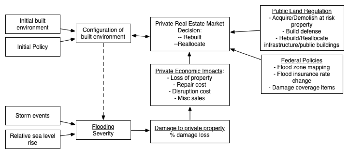
Figure 1. Scope of Coastal Real Estate Market Adaptation Model

The Model

2.1

Previous relevant agent-based models have emphasized emergent urban form at the metropolitan scale (Xie, Batty & Zhao 2007), coastal adaptation at the landscape scale (Simoes et al 2009), financial shocks in housing markets (Gilbert, Hawkesworth & Swinney 2009), and metropolitan land market dynamics (Zhou & Kokelman 2011). Our model focuses on storm-related shocks in a local, coastal housing market. The model is constructed using NetLogo (Tisue & Wilensky 2004; Wilensky 1999).

2.2

The model is calibrated to the real property of Highlands and consists of 2,617 parcels (Monmouth County 2013) that we have distributed over a 55 × 55 pixels grid. Our stylized topography has low-lying, medium, and high-elevation areas (see Figure 2). Based on elevation and amenity, parcels can be grouped into four categories:

• Waterfront Lots consist of 534 parcels in the first row of the grid that is adjacent to the shoreline;
• Flood-zone Lots consist of 849 parcels that are located in sections of the grid located in low-lying areas that do not have a water view;
• Elevated Lots consist of 271 parcels located in medium-elevation areas that do not have a good water view;
• Water-view Lots consist of 963 parcels located at higher elevations compared to other lots. These lots have a good water view and each grid cell is ten feet higher than the lower grid cell next to it closer to the shoreline.

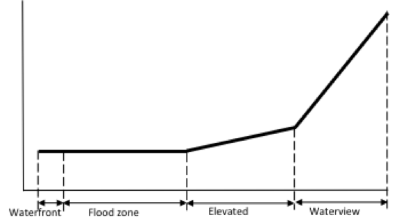
Figure 2. Topography of Stylized Coastal Town

Agents

2.3

The model consists of three types of agents: Households, Bank, and Parcels.

Households

2.4

Based on Households' activities in the real estate market, we group them into three categories: Homebuyers, Homesellers, and Homeowners. Each unit of time or "tick" represents one year. Each year, homebuyers search for properties available in the town. Initially, homebuyers look for houses and if there are no houses available, they start looking for empty lots. Homebuyers consider buying properties firstly from private sellers, then from a bank. Homebuyers consider geographical location in buying properties. Properties located on the waterfront are the most desired ones, followed by the properties having a water-view or located in an elevated zone, and the least desired ones are properties located in the flood zone. Homebuyers also prefer properties with the highest price that is affordable to them. Home purchases are financed with 30-year fixed-rate mortgages.

2.5

Homebuyers are given a maximum of three years to look for a desired property before they are forced to leave the market. Upon buying of a property, homebuyers move into the town and become homeowners. The length of owning properties depends on their income level, that may fluctuate ranging up to ± 20%, which determines whether they can afford to continue paying the mortgage or not. Repair or rebuilding costs resulting from flood events must be paid in order for homeowners to keep their properties. If they can no longer afford to pay all the required costs, they will be forced to sell their property. Foreclosure occurs if after 3 consecutive years the unaffordable property is still on the market. Homesellers may also sell their properties if the opportunity arises to make windfall profits or if they must move out of town due to reasons unrelated to real estate (U.S. Census Wealth 2013). If homesellers stayed in the market permanently, the market would collect poor people, causing numbers of transactions to drop. So, the model forces people out after 3 years to preserve the full income distributions among buyers.

2.6

This model also implements a social influence concept, where homebuyers influence each other in seeking adaptive strategies (renovate, elevate, and sell). A homeowner's decision to elevate the house influences other homeowners who live within a certain buffer to perform the same action. Social influence can be modeled using three network approaches. A scale-free network explains the emergence of vertices (or hubs) with a number of connected edges that exceed the average (Deffuant et al. 2000; Wang & Chen 2003). Accordingly, this approach does not sufficiently explain how it affects the outcomes (e.g. housing prices and vacancy rates). A small-world network might be useful to explain social influence through the identification of hubs and sub-networks that emerge; however, this approach still does not affect the outcomes. The last approach is that adopted by the model, and considers all households to have the same power to influence their neighbors albeit with distance decay. A household has the greatest influence to its closest neighbors and the smallest influence on the most distant ones.

Bank

2.7

The bank agent in this model possesses fewer roles than the traditional banks we know in the real world. The bank agent, however, channels the modeler's power in parsimoniously maintaining the simulation dynamic. For example, the bank initially owns all parcels that homebuyers buy. Its presence simplifies the complexity of having individual agents ownership at the initialization, which may result a more patchy or clustered development. The bank also takes foreclosed homes from homeowners who can no longer afford to keep their homes. This is to damp down the potential "death spiral" dynamic of property prices in a self-regulating market, a role evident in U.S. post-disaster banking practices. The bank sells these properties at non-negotiable prices. Like sales made between homebuyers and home sellers, sales by the bank also contribute to the housing market performance in the region. Therefore, sales of large numbers of foreclosed houses significantly affect housing prices in the area. House values (building and land values) are adjusted due to these activities.

Parcels

2.8

The simulation starts with an empty town in which all land lots, parcels, belong to the bank. Land lots have attributes including land type, elevation, and land_value. The land type attribute refers to the four types of categories of a property discussed above. Elevation refers to the z-axis of the location of the land lot. The z-axis equals to zero at sea level. Initially, all land lots have the same land value of $5000. Demand-supply principles of economics apply to adjust the land values. This is reflected in the transaction prices agreed between homebuyers and homesellers (or the bank).

2.9

In our model, all houses are single-family detached houses that have similar construction. Based on 2010 CENSUS, the median housing value in Highlands, NJ is $219,000. We calibrate the model with assessed property value data, and in Highlands the mean ratio of building value to total assessed value (land plus improvements) is 0.46 (S.D. 0.14) (Monmouth County 2013).

2.10

Each year, homeowners decide either to maintain their homes based on their ability to pay repair fees, and if they cannot afford it they let the houses depreciate in value. In a post-flood event, homeowners may also decide to (1) repair or (2) elevate the house up to ten feet above the ground to reduce future flooding risk. The cost to elevate a house is 50% of the building value. Some homeowners who have suffered flooding damages invest in elevating their homes by taking out a second mortgage. This second-mortgage payback period is set to 15 years.

Flooding

2.11

Flood loss estimation is calculated based on three sub-modules: an annual probability distribution of local flood depths, a stage-damage function that calculates the damage percentage at a given flood level, and an economic module to convert a damage level into a monetary loss (Figure 3) (Grigg & Helweg 1975; Kang, Su & Chang 2005).

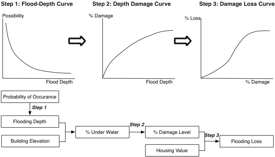
Figure 3. Flooding Damage Calculation Flow Chart.

2.12

A probabilistic Flood-Depth Curve represents the probability distribution of flood events with particular water depths. The distribution used in the calibrated model is based on historical annual high-water exceedance probabilities for adjacent Sandy Hook, NJ (NOAA 2013). Also, we assume the flooding depth is 0.1 feet for a one-year flood event and 10.05 feet for a 500-year level flood level to keep the curve-fitting simple. A logarithmic model fits the historical data well (see Figure 4). In our model, one random flood event is generated annually. Thus, the model calculates the flood depth based on the possibility generated by our model. The general model to calculate the probability of flood occurrence:

f(x) = 2.781 × e−0.6039x x = flood depth

(1)

2.13

A Depth-Damage Curve relates flood damage to flood inundation parameters for residential buildings. Flooding inundation parameters such as construction details, flood depth, duration, and velocity all affect damage level. Only the relationship between flood depth and damage level is considered in the model. Flood depth starts as a negative number because it is defined relative to the floor of the inhabited space, not the ground level. The general flood depth-damage curve model shown in Figure 5 is based on FEMA (2013):

f(x) = 170 × (1 − e(−a × (x + b))) Coefficients (with 95% confidence bounds) a = 0.0302 (0.02959, 0.0308) b = 3.976 (3.724, 4.229)

(2)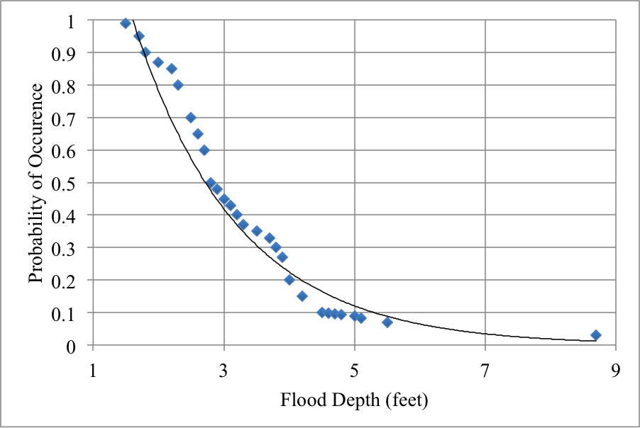

Figure 4. Flooding Possibility Depth Curve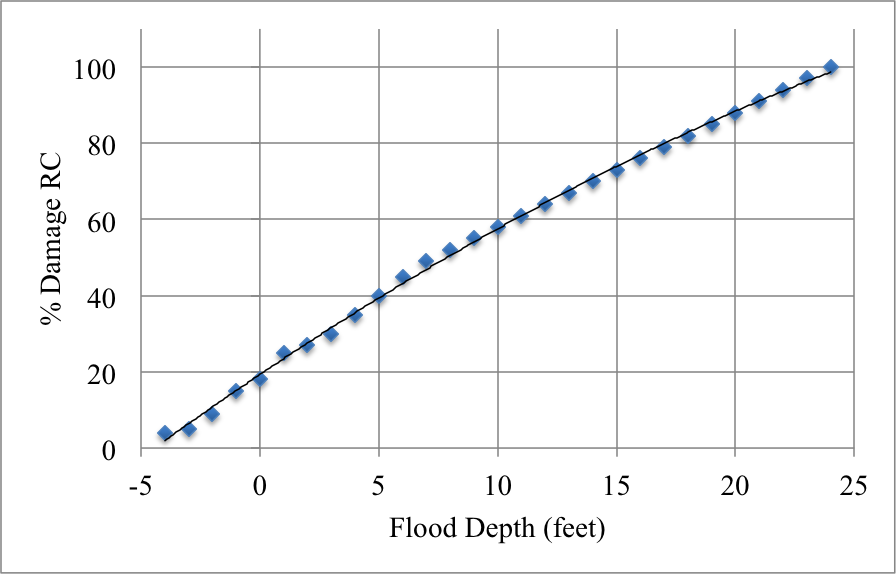

Figure 5. Flood Depth Damage Curve

2.14

A Damage Loss Curve: Homeowners only consider the loss of a damaged building structure whenever there is a flood event. Loss of building contents is not included in the model. The model assumes Loss = %damage × Building Value.

Double Auction Market

2.15

In modeling the interaction between private homesellers and homebuyers, this model adopts the experimental economics of double auction markets. The goal of this approach is to achieve high levels of market efficiency quickly by running rounds of trading between buyers and sellers. Similar to experiments conducted by Gode and Sunder (1993), this model provides three choices: bid, ask, and transaction. Whenever a bid and ask cross, the transaction price is equal to the earlier of the two. Thus, there are four possible states: 1) no best ask (lowest ask price) nor a best bid (highest bid price); 2) a best ask and no best bid; 3) no best ask but a best bid; or 4) both a best ask and best bid.

2.16

This model, however, extends the previous double auction market model by introducing the role of a bank in a minimal form. A bank has similar characteristics to private sellers: it makes an offer and can contribute to the overall market price. It, however, does not have an auction mechanism with buyers. Homebuyers buy homes from a bank whenever they cannot find the desired properties offered by private sellers.

2.17

Initially, a homebuyer forms a bid price between his income level, adjusted by an affordability multiplier, and zero. A home seller randomly forms an ask price between the maximum reasonable market price and his buying price of the property. A selected homebuyer then compares his bid with the best ask. If his bid is above the best ask, he accepts the best ask and the transaction occurs at the best ask. If his bid is below the best ask (or there is no best ask) and there is no best bid, it becomes the best bid. If his bid is below the best ask (or there is no best ask) and above the best bid, it overrides the best bid. If his bid is below the best bid, the bid is ignored. The rule also applies to a selected homeseller. If his ask is below the best bid, a trade occurs at the best bid. A homeseller and a homebuyer that make a successful transaction are removed from future trading. The process continues until there are no longer sellers or buyers that can make offers in the market.

Modeling Framework

2.18

In general, this model simulates households' movement logic into and out of a coastal town. Figure 6 shows the process of the real estate market.

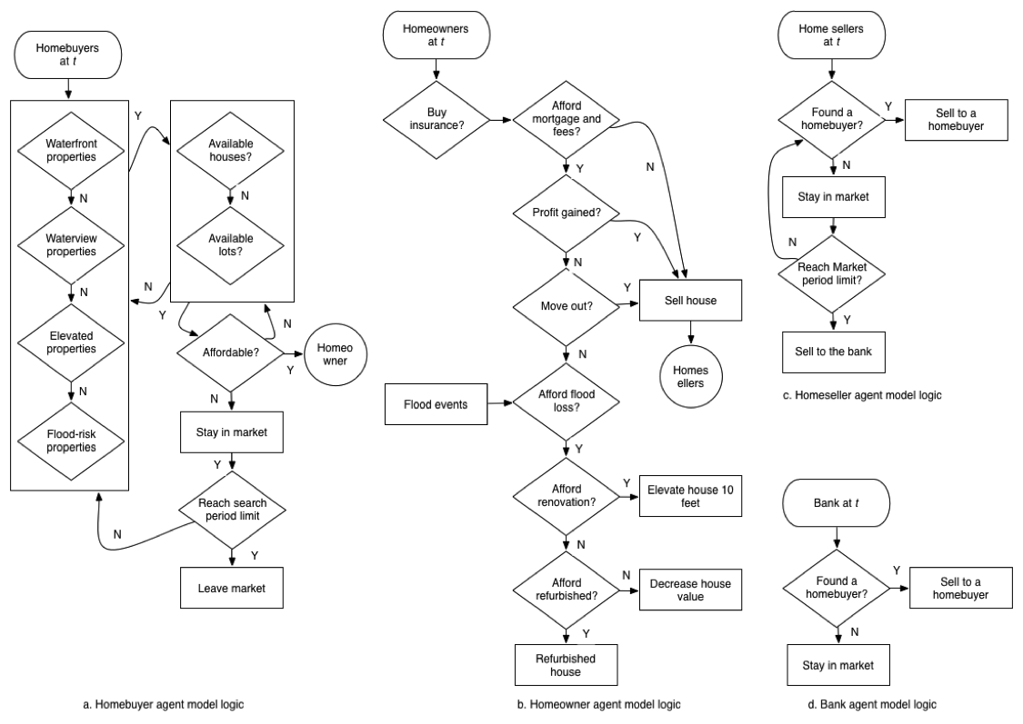
Figure 6. Modeling Framework

Buying decision

2.19

A number of homebuyers enter into the town annually to look for their ideal homes. Following U.S. convention, when homebuyers decide on the affordability of houses, their expected annual payment for housing needs to be lower than 30% of their annual income. The 30% rule of thumb is based on the U.S. convention as being the reasonable amount of income to be allocated for housing (FHA 2014):

(30% × Income) ≥ (Mortgage + Property Tax)

(3)

2.20

Here, the annual mortgage calculation is based on Eq. 4.

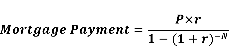
(4)

where:

N is the loan's term, the number of yearly payments. Our initial setting of mortgage duration is 30 years;
r is the annual interest rate;
P is the loan's principal, the amount borrowed from bank. We assume every homebuyer can afford a 15% down payment. They need to borrow 85% of the housing price from the bank.

2.21

The property tax calculation is based on the market value of the house (Eq. 5).

Property Tax = Tax Rate × Housing Price

(5)

(5)

2.22

In 2010, the property tax rate for the case study town is 2.55% in Highlands, measured as the percent of assessed value paid annually in taxes. When homebuyers have foresight about future flooding risks, they also consider potential flooding losses to check whether the house is affordable (see Eq. 6).

(30% × Income) ≥ (Mortgage + Property Tax + Flood Insurance + Annual Expected Uninsured Flood Loss)

(6)

2.23

The calculation of expected flood loss is based on a 100-year flood event (p = 0.01).

Annual Expected Flood Loss = 0.01 × (Flooding Loss of 100 Year Storm).

Selling decision

2.24

Homeowners keep their houses based on their ability to pay the monthly mortgage and other costs. Unlike homebuyers, homeowners try to keep their homes. They are willing to pay up to 50% of their annual income for housing-related costs. If they cannot afford to pay the housing costs for more than 3 years, they will finally give up by selling their houses and moving out (Eq. 7). The U.S. median household net-worth data shows a typical amount of saving that is sufficient to pay 3-year of mortgage (U.S. Census Wealth 2013).

(50% × Income) ≥ (Mortgage + Property Tax + Flood Insurance + Annual Expected Uninsured Flood Loss)

(7)

2.25

Even if homeowners can afford to pay their housing related costs, homeowners may move out from their homes due to personal reasons. Another reason is to sell the property for a windfall profit.

Flooding Insurance

2.26

Flood insurance premiums are calculated based on factors such as year of construction, building occupancy, number of floors, location of contents, flooding risk, location of the lowest floor in relation to the elevation requirement on the flood insurance map, and housing value (FloodSmartgov 2013a). Table 1 shows a sampling of flood insurance premiums in different flood risk areas.

Table 1: Sampling of Policy Premiums for Qualified Structures with Basement or Enclosures in the National Flood Insurance Program (FloodSmartgov 2013b)
Building & Contents	Moderate to Low Risk (NFIP Zone B, C, X)	High Risk Area
	Preferred Rate	Standard Rate	Preferred Rate	Standard Rate
$150,000/$50,000	343	1263	1695	3270
$250,000/$100,000	365	1717	2930	6410

2.27

In the model, we use Premium-to-Loss Ratio and Annual Expected Flood Loss to calculate flood insurance for each house. This will highlight the effect of flooding risk. Premium-to-Loss Ratio is the ratio of flood insurance premium to expected annual flooding loss. An adjustable slider is set up on the modeling interface to test the impact of different rates of Premium-to-Loss Ratio (Eq. 8).

Flood Insurance = Premium-to-Loss Ratio × Annual Expected Flood Loss

(8)

Federal flood insurance policies cover physical damages to houses and personal property. As a basis for comparing behavior given the coverage and federal requirements of the flood insurance program, we adopt a contrasting free-market scenario to test how changes in NFIP affect the coastal real-estate market.

2.28

The free-market scenario is the basic flood insurance scenario in the model. Only homeowners who have foresight regarding future flood risk will consider buying flood insurance. Their decision is based on the Premium-to-Loss Ratio. If Premium-to-Loss Ratio ≤ 1, foresighted households will buy flood insurance (Eq. 9). When a flood event happens, flood insurance will cover all the flood losses for insured houses. For houses without flooding insurance, residents need to pay all of the flood-related loss. These households will get loans from the bank to pay off all the flooding recovery cost. In our model, the mortgage duration for this type of loan is 15 years.

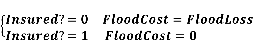
(9)

Results

3.1

We show two sets of results. The first set demonstrates the model's face validity by reproducing dynamics commonly seen in the real estate marketplace within the Highlands empirical context. The second set of results explores policy alternatives.

Validation

3.2

For validation, we simulate the New Jersey experience during the twenty-year span from 1988 to 2007. Homebuyers search for homes according to their preferred locations. Figure 7 shows results that are consistent with the assumption that homebuyers initially search for their desired homes in the waterfront zone, followed by waterview zone, and elevated zone, with the flood zone being the least desired location.

3.3

Rather than drive the model with flood events drawn randomly from a probability distribution, for validation we specify a set of flood events reflecting the New Jersey record from 1988 to 2007 (NOAA 2013). Figure 8 shows this pattern of flooding.

3.4

These flood events cause significant damage to coastal homes. Figure 9 shows the timeline of damage and its intricate relationship with the timing of home construction in each zone. Waterfront properties, built earliest, suffer damage in year 3, after which many owners elevate their structures, so that they are less vulnerable during later floods. Development next occurs on parcels not vulnerable to flooding, first in areas with water views, and then in elevated but view-less areas. Development in the flood zone commences in year 6 and concludes in year 9, just in time to suffer significant damage during storms in years 10 and 12. A wave of waterfront rebuilding in years 10 to 14 is mostly built to a higher standard, reflecting awareness of flood risks, but the overall flood damage in year 15 is the highest yet.

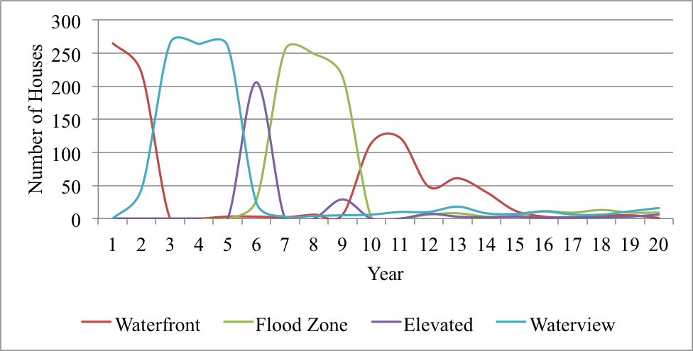
Figure 7. Total number of houses built over time.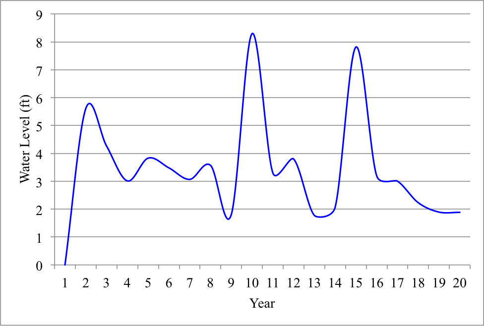

Figure 8. Flood depth over time (in feet).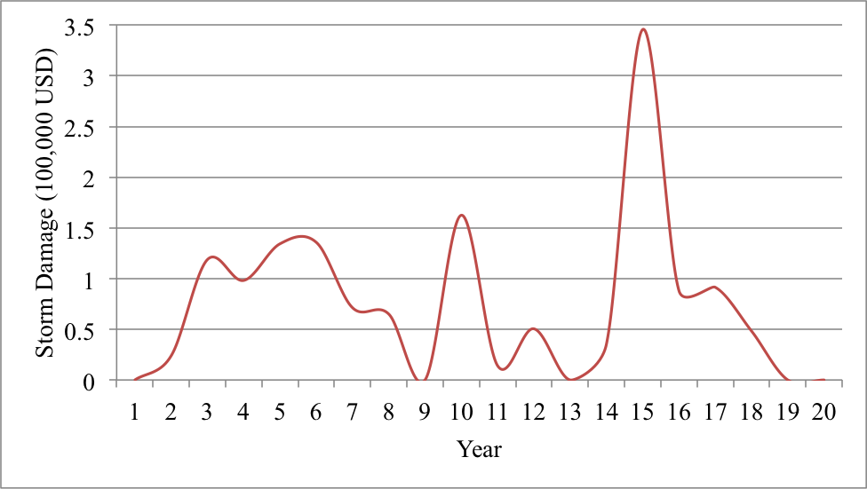

Figure 9. Total value of flooding damage over time (100,000 USD).

3.5

The double auction market allows housing prices to emerge from the interactions among homebuyers, home sellers, and flooding events. In the model, homebuyers may visit up to 30 houses before deciding to buy their desired house. It is difficult to interpret the trend movement of these transactions. Figure 10 shows that transaction prices for homes in the risky, amenity-rich waterfront zone start higher than for houses located in the other zones, but that prices for water-view houses outside the floodplain eventually overtake them. These two submarkets are clearly linked, as shown by the dip in prices for waterview homes in response to the spurt of rebuilding in waterfront homes in year 12. House prices in the flood zone remain persistently lower than those in the elevated zone. Housing prices regularly dip at about three years after major storms, as homeowners who are struggling financially finally give up their homes.

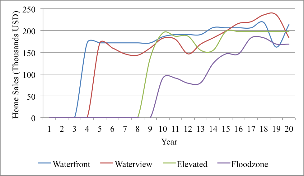
Figure 10. Annual average value of home sales over time.

3.6

There is a correlation between homeowners' ability to anticipate flood events and their foreclosure market behavior. Figure 11 shows how foresighted homeowners suffer less from having their houses foreclosed, indicating that they have a safety net, insurance, to pay their flooding loss. In contrast, many homeowners who do not foresee these flood events have to let their houses go into foreclosure.

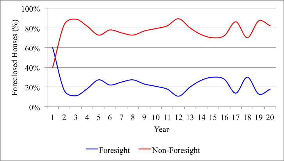
Figure 11. Percent of foreclosed houses by types of homeowner (i.e. foresight, non-foresight) over time.

Policy Scenarios

3.7

Table 2 shows that the next set of results examines the impacts of four policy scenarios, followed by two sensitivity runs testing the implications of key assumptions. Policy scenario #1, "Foresight," assumes that only homeowners who have the foresight to anticipate the possibility of flooding bother to buy flood insurance; no one is required to do so. Policy scenario #2, "100-year Flood Zone," requires all homeowners living within the 100-year flood zone to buy flood insurance, and it covers 100% of losses. Policy scenario #3, "80% Reimbursement," requires that all homeowners living within the 100-year flood zone must buy insurance, but the insurance only reimburses 80% of the losses suffered and it only does so for substantially damaged buildings where losses exceed 50% of the building's value. Policy scenario #4, "Cap Reimbursement," requires that all homeowners living within the 100-year flood zone must buy flood insurance, but the insurance only reimburses losses up to a cap amount of $100,000.

3.8

The next two scenarios examine the effects of key parameters. Scenario 5, "Cap Reimbursement assuming contagion," deviates from Scenario 4 by assuming that homeowners have a high (instead of zero) probability of influencing their neighbors in regards to their post-flood adaptation decisions (e.g. sell, elevate). Scenario 6, "Cap Reimbursement assuming higher incomes," varies Scenario 4 by assuming that a large fraction (50% instead of 2%) of home buyers are wealthy.

Table 2: A summary of policy scenarios developed in the study.
#	Insurance policy	Influence level	% Hi Income population
1.	Foresight	None	2%
2.	100-year Floodzone	None	2%
3.	80% Reimbursement	None	2%
4.	Cap Reimbursement	None	2%
5.	Cap Reimbursement, and 50% influence level	50%	2%
6.	Cap Reimbursement, and 50% high-income home buyers	None	50%
7.	Limit years period to sell properties (3-year vs. no limit)	50%	50%
8.	Household income variability (0% vs. 20%)	50%	50%

3.9

Figure 12 shows that the 100-year Floodzone scenario (#2) with a mandatory insurance requirement for houses in the 100-year flood zone yields lower uninsured damage costs than the Foresight scenario (#1) in which insurance is voluntary.

3.10

Figure 13 shows the implications of alternative reimbursement arrangements in the flood insurance program. Scenario #2 (100-year Floodzone) reimburses 100% of insured losses and thereby keeps uninsured damage costs low until the town is fully built out (year 14), after which costs become much more volatile. Scenario #3 (80% Reimbursement) reimburses only 80% of damage costs and then only for houses with significant damage, and the result is that uninsured losses are much higher and amounts are volatile. Scenario #4 (Cap Reimbursement) only reimburses damage costs up to a maximum of $100,000, and the result is very modest volatility and low uninsured damage costs, because homeowners and home buyers internalize more of the risk in their own calculations, albeit with a delay.

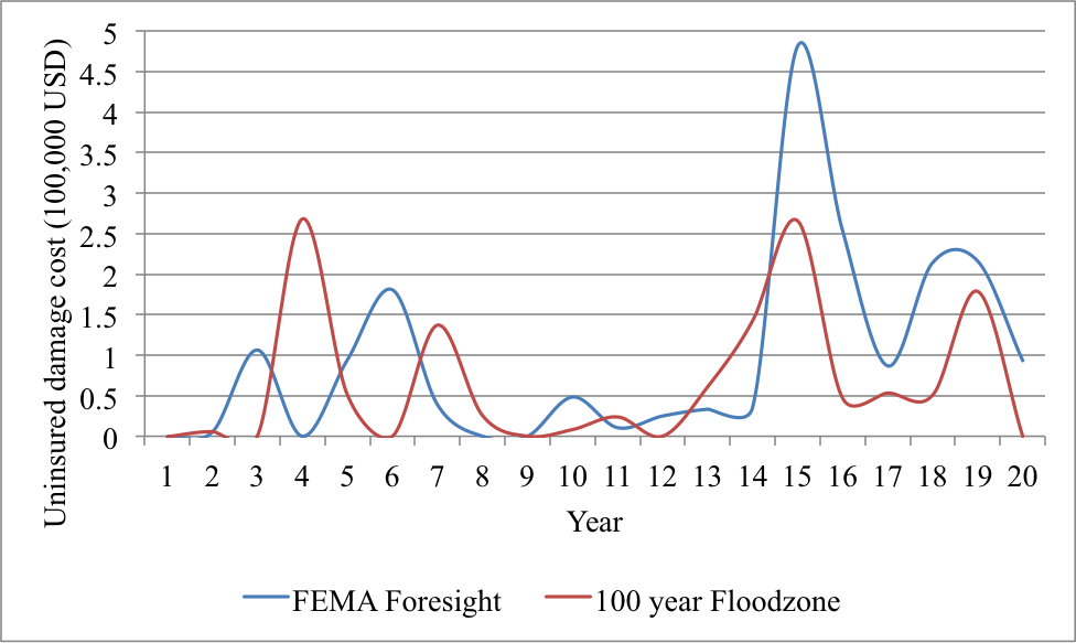
Figure 12. The impact of voluntary (#1) versus mandatory (#2) insurance scenarios on flood damage costs over time.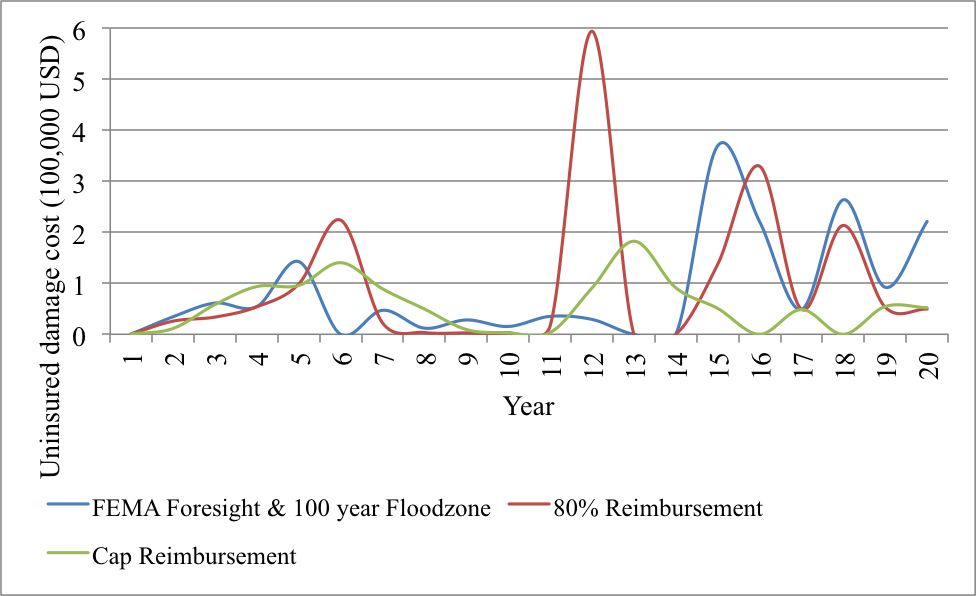

Figure 13. The impact of different insurance reimbursement arrangements (scenarios #2, #3, #4) on flood damage cost over time.

3.11

Figure 14 shows how homeowners influence their neighbors in making decisions such as selling or elevating their houses, and how it affects home sales prices. The simulation results are consistent with a modeling logic wherein more sellers tend to decrease the prices. Home sellers in a scenario that allows contagion tend to sell their houses at lower prices than home sellers in a scenario that does not allow contagion. Moreover, the experiment indicates that the vacancy rate in the contagion scenario is relatively higher at 7% than in the scenario without contagion at 1% (see Table 3).

Table 3: Impact of social influence on home sales and vacancy rates
	With Contagion	Without Contagion
	Median	Mean	Median	Mean
Home Sales	$157,641	$151,235	$175,386	$164,072
Vacancy Rate	6.8%	7.9%	1%	1%

3.12

Figure 15 shows the results of the final experiment, which is to change the income distribution of the home buying population. While only 2% of the population in Scenario #4 has a high income, Scenario #4h allows 50% of the population to have a higher income. The results confirm that higher home sales prices are the likely result. This fits an observed pattern of gentrification of the shore within well-connected metropolitan areas, in which higher-income households displace lower-income households following expensive storm damage.

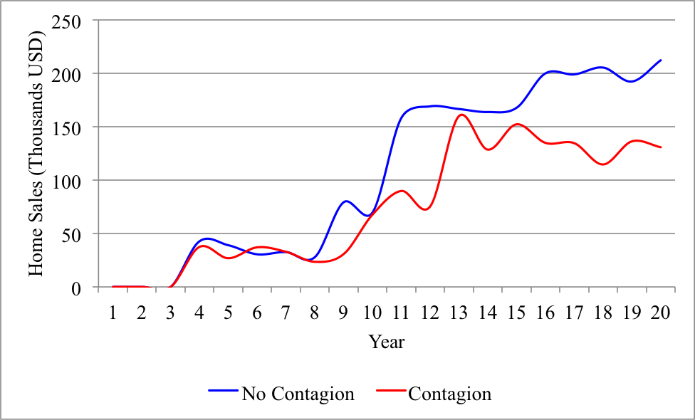
Figure 14. The impact of social influence on home sales over time.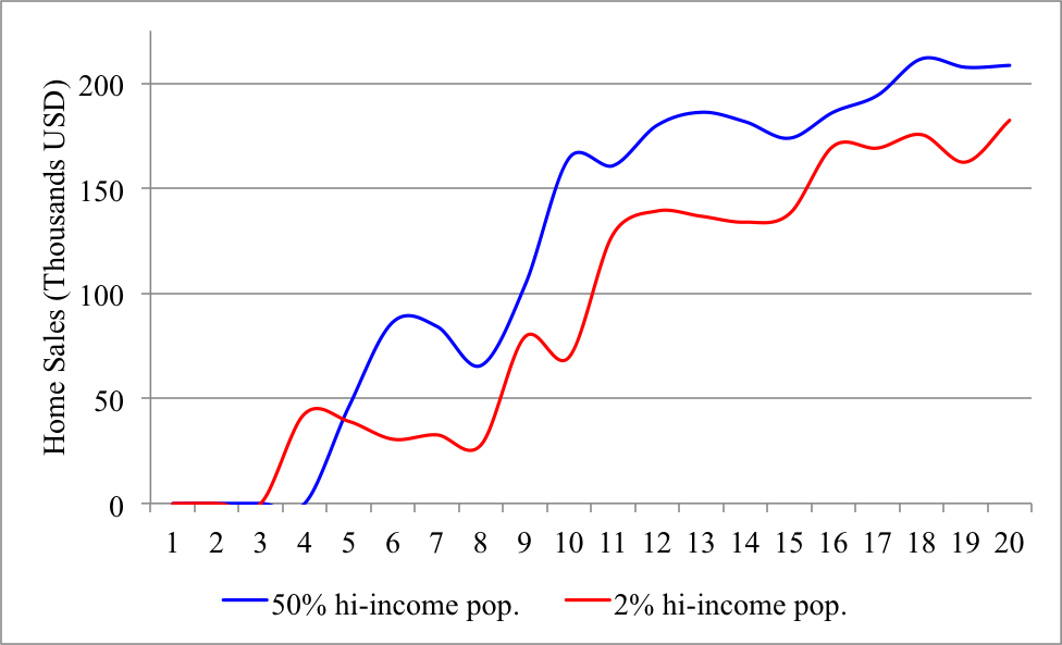

Figure 15. The impact of income level on home sales over time.

3.13

The next scenario is to show the effect of the limit year period for home sellers to sell their houses before going to foreclosure on home sales. Figure 16 shows how the 3-year limit (U.S. Census Wealth 2013) is necessary to prevent home sales from spiraling down. Home sales decrease in prices significantly after year 14 in the scenario without years limit, while it remains stable in a scenario with the 3-year limit period.

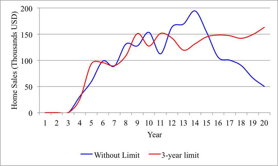
Figure 16. The impact of years limit on home sales over time.

3.14

The effect of income variability over time consistently shows its effects on foreclosure pattern as well as home sales patterns. Figure 17 compares a model with 20% variability on household's income to a model without any household income variability. Foreclosures do not necessarily push the prices downward. This is because more transactions occur that encourage home seekers to make offers. Home seekers with high income stay longer and increase their offer as they have more purchasing power than home seekers with lower income.

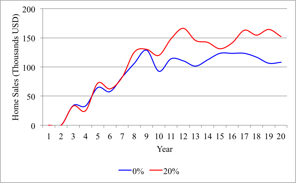
Figure 17. The impact of household income variability on home sales over time.

3.15

Figure 18 shows that the policy scenarios correlate only modestly with the observed historical house sales price trend from Highlands. Although the model captures the upward trend in housing prices, it misses key exogenous drivers of local housing prices including the 2000–2008 national housing bubble. In the early years of the simulations, it unrealistically assumes an empty landscape, whereas the real town was fully built out by 1980.

3.16

Overall, the ten models are only modestly calibrated with the historical home sales data from year 1988 to year 2007 (Figure 18). While the model is limited from other factors such as housing bubble phenomena and accurate homeowners behaviors, the models reflect the increasing trend of historical home sales data.

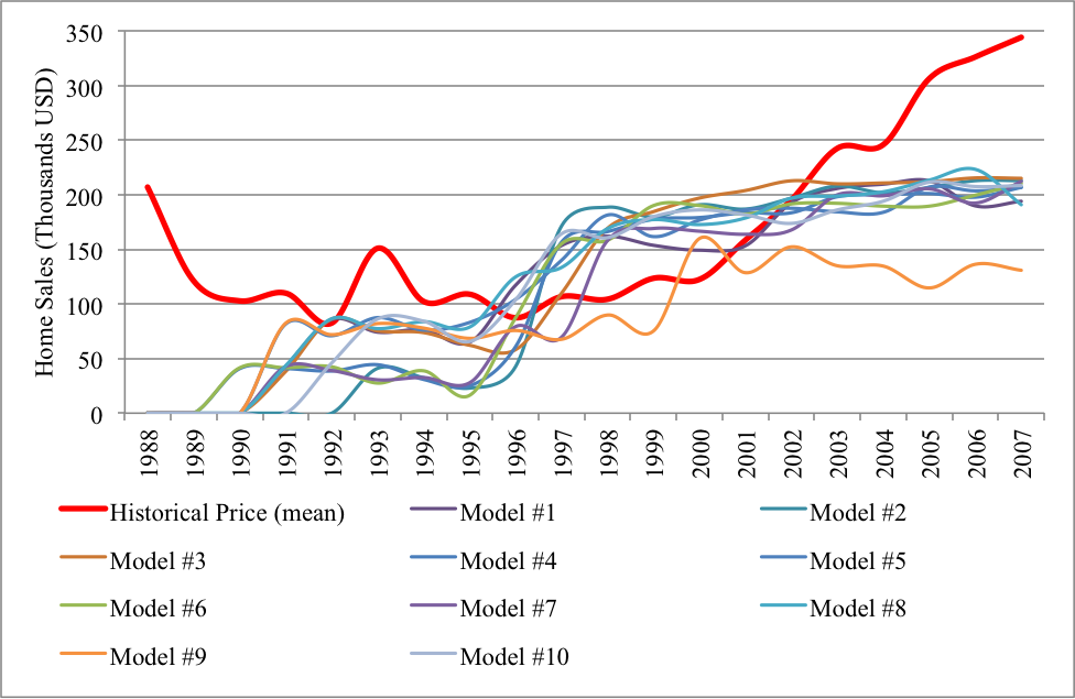
Figure 18. Comparative home sales data for ten models.

Conclusion

4.1

This study has demonstrated a plausible modeling logic that captures essential features of residential real estate markets in vulnerable coastal areas. The study also provides a basic calibration of the model with local home sales price data, a strong validation its internal logic, investigation of additional policy scenarios beyond the laissez faire base case, and analysis of its sensitivities to key assumptions. Future research could develop a model of a complete real estate market including national market trends and residential, commercial, and industrial properties; validate the model in additional municipalities; parsimoniously scale up the model for use in regional analysis; and extend the model to include municipal decision making.

Addendum: The ODD Protocol^[1]

1 Purpose

The purpose of the model is to investigate the adaptive responses of real estate markets to changing patterns of flooding and flood insurance policies by means of parallel theoretical and empirical efforts.

2 Entities, state variables, and scales

Agents/individuals. The model has different types of agents.

• Household are categorized into three different groups: Homebuyers, Homesellers, and Homeowners. Household has attributes as follow:
    — color                           ; color id
    — income                        ; income (usd)
    — best_house                  ; best house yet found
    — person_land                ; connecting land
    — person_house              ; connecting house
    — search_time                 ; time period a homebuyer searching for a desired property
    — stay_time                     ; time period a homeowner owning a property
    — warning_time              ; time period a homeowner to pay the annual fees
    — selling_time                 ; time period a homeseller to sell the property
    — floodFree_Preferred? ; a homebuyer preference on a property location
    — traded?                        ; if a homebuyer/a homeseller already make a trade or not
    — annual_fee                   ; amount of annual fee need to be paid by a homeowner (usd)

• Bank owns all empty lots and foreclosed homes. Bank has attributes as follow:
    — person_land   ; connecting land
    — person_house ; connecting house
    — traded?           ; if a bank already make a trade or not

• Houses are dwellings built on top of land patches. Houses are attributed with:
    — house_person   ; connecting person
    — house_land       ; connecting land
    — elevated?          ; if the building is elevated or not
    — building_value ; building value (usd)
    — onmarket?        ; if the house is available in the market or not
    — property_tax    ; property tax (usd)
    — fees_duration   ; duration of mortgage
    — floodingloss     ; amount of loss because of flood events (usd)
    — insured?           ; if the building is insured or not

• Spatial units are pixel grid cells with attributes as follow:
    — land_person  ; connecting person
    — land_house   ; connecting house
    — land_type      ; type of land (e.g. waterfront, floodzone, elevated, waterview)
    — elevation       ; elevation (feet)
    — land_value    ; land value (usd)

Environment. The model has two types of environmental variables.

• Economic variables: market price, insurance fees, mortgage fees, flooding loss
• Environmental variables: flooding events, flood depth
• Collectives. The model has seven agentsets, collections of agents.
• Homebuyers                 ; households who take roles as homebuyers
• Homeowners                ; households who take roles as homeowners
• Homesellers                 ; households who take roles as homesellers
• Waterfront_properties ; houses and lots located at the waterfront zones (the first row pixel grid)
• Floodzone_properties  ; houses and lots located at the floodzones and without waterview
• Elevated_properties     ; houses and lots located at the higher ground but without waterview
• Waterview_properties  ; houses and lots located at the higher ground and with waterview

One time step represents one year and simulations were run both for 50 years and 200 years. One grid represents 1 parcel and the model comprised of 2,617 parcel data.

3 Process overview and scheduling

to setup
  setup-global-variables
  get-input-files
  setup-land-patches
  setup-houses
end

to go
  while [ticks < MAX_TICKS] [
    reset-output-parameters
    flood-event
    house-process
    market-process
    data-store
    tick
  ]
  data-output
end

to person-process
  setup-persons
  ask persons [
    ifelse homebuyer [
      set search_time ++
      if search-time > BuyerSearchLength [ leave-market ]
    ]
    [ if homeseller OR bank [
      income-shock
      maintain-house
    ]
  ]
end

to house-process
  ask houses [
    if owned [
      agingrepair
      floodrepair
      elevate
      fee-add
  ]
]
end
to market-process
  setup-banks
  let market_type 0      ;;; 0-waterfront 1-floodzone 2-elevated 3-waterview
  while [market_type < 4] [
      market-run
      landvalue-update
      set market_type (market_type++)
  ]
  reset-banks
end

4 Design concepts

Basic principles. The model adopts a microeconomics model of a double auction market and expands it by incorporating several different markets and externalities such as price restriction by the government agent.

Emergence. Transaction prices and homeowners' selling behaviors are modeled as emerging from the adaptive traits of household agents. These results are expected to vary in complex and perhaps unpredictable ways when the agents' characteristics as well as the surrounding environment change. Results pertaining to the environment are not emerging such as the initial moving in patterns. Homebuyers initially buy lots located at the waterfront zones, then waterview zones, then elevated zones, and lastly lots located at the floodzones.

Adaptation. Homebuyers who consider flooding risk by purchasing flood insurance will not experience great loss from the flood events. Homebuyers buy the highest price affordable to maximize property values at the least cost possible. Homebuyers prefer to buy homes located in the waterfront and waterview zones providing better property values. Homeowners who elevate their homes suffer less damage from the future flood events.

Objectives. Homebuyers' objective is to get the best affordable properties. Homeowners' objective is to pay the least possible mortgage and other annual fees in order to keep the properties as long as they can. Homesellers' objective is to sell above the market price. Government' objective is to protect housing market values by making flooding adaptive actions such as mandating homeowners to elevate their homes and to buy flood insurance.

Learning. Homeowners who previously did not consider flooding risk, buy flood insurance and elevate their homes upon the occurrence of flood event.

Prediction. Homebuyers who buy flood insurance have the ability to anticipate without precisely predicting future flood events. The timing for homeowners to sell their homes at profit shows the ability to predict future housing market prices.

Sensing. A homebuyer enters the housing market sensing the availability of properties that best fit his locational preference and income. A homebuyer makes a bid based on his ability to afford the property and the best offer in the market. The mechanisms by which agents obtain information are modeled explicitly, and they make decisions based on these rules and mechanisms.

Interaction. Homebuyers compete with each other in looking for their desired properties. The same rule also applies to homeowners who are trying to sell their properties. Auction model is the mechanism used to represent the communication between homebuyers and homesellers.

Stochasticity. Flood events are measured stochastically with certain probability.

Collectives. The four housing markets in the model determine the grouping of homeowners. Transactions between homebuyers and homesellers in a single market determine the housing market price, building values, and land values of all properties in the market.

Observation. Data are collected in yearly basis. Data included are flood depth, storm damage (usd), percent damage, sell high for profit, sell low due to affordability, number of sales by bank, number of sales by private sellers, building value, land value, vacancy rate, transaction price, home buyers income level.

5 Initialization

The initial state of the world is at time t = 0 of a simulation run. Each time tick represents one year. A housing parcel data consisting 2,617 parcels are distributed over 55 x 55 pixels grid, land patches. The model topography has low-lying, medium, and high-elevation zones. Based on elevation parcels are grouped into three categories: waterfront lots consist of 534 parcels are located at the first low grid that adjacent to the shoreline, floodzone lots consist of 849 parcels are located on grids also at the low-lying areas, elevated lots consist of 271 parcels is the medium elevated area, and waterview lots consists of 963 parcels are located in the higher points compare to other lots' types locations. There were no houses on top of these land patches.

Each year, 600 homebuyers enter into the market. The values of their attributes are: traded?=false, search_time=stay_time=warning_time=0, person_house=nobody, person_land=nobody.

6 Input data

The model use input from a data file of Highlands, NJ parcel data to represent processes. This data is also used for calibrating and validating the model.

7 Submodels

Each time tick represents one year. Each year, the model runs processes as follow:

• Setup                                ; setup all necessary variables
  — setup-globalvars         ; setup all global variables
  — data-input                   ; read input files
  — setup-patches              ; setup land patches 55 × 55 pixel grid
  — setup-houses               ; setup all houses variables (not included initially)
  — dataparcel-get            ; read particular parcel data

• go                                     ; run simulation iteratively at every time tick
  — reset-outputparams     ; reset all output parameters
  — flood-event                  ; run random flooding events
  — house-process             ; run processes for all houses
    ∘ house-agingfix            ; homeowners repair houses due to aging
    ∘ house-floodrepair       ; homeowners repair houses due to flooding
    ∘ house-elevate              ; homeowners elevate houses
    ∘ fee-add                        ; add a necessary fee need to be paid by a homeowner
    ∘ fee-decrduration         ; determine the duration for a fee
    ∘ house-sell                    ; run sell process
  — person-process            ; run processes for all persons
    ∘ setup-persons              ; setup persons' variables
    ∘ income-shock              ; run random income shocks to homeowners
    ∘ maintain-house            ; run maintain house processes for homeowners
  — market-process            ; run double auction market
    ∘ bankagents-setup         ; setup banks agents to handle all unowned properties
    ∘ market-run                  ; run market processes
      ∎ buyers-initial            ; initiate buyers' variables
      ∎ sellers-initial            ; initiate sellers' variables
      ∎ trading-initial           ; initiate order book used for trading mechanism
      ∎ doTrade                    ; run trading processes between homebuyers and homesellers
        ∘ formBidPrice           ; assign random bid offers to home buyers
        ∘ formAskPrice           ; assign random ask prices to home sellers
        ∘ traders-traded          ; finalize successful traders
      ∎ transPrice-set           ; set transaction market price if a trade is successful
        ∘ traders-update         ; homeowners can make transactions
          ∎ buy-property-deal ; finalize the purchase
          ∎ property-better-affordable ; if the property in question has the highest affordable price tag
          ∎ buy-property-from-bank ; homeowners buy properties from a bank
      ∎sellersbank-buy          ; run a process for homeowners to buy properties from a bank
    ∘ landvalue-update         ; update land value caused by the transaction
    ∘ bankagents-reset          ; remove all bank agents from the model at the end of every time tick
  — data-store                     ; store all output data into an array
  — data-output                   ; print all output data into a file )

Notes

¹See Grimm et al. (2010).

References

BAGLEY, K. (2013). Climate change impacts absent from FEMA's redrawn NYC flood maps. Inside Climate News. Available at http://insideclimatenews.org/news/20130204/climate-change-global-warming-flood-zone-hurricane-sandy-new-york-city-fema-federal-maps-revised-sea-level-rise Last Accessed in April 2013.

BINDOFF, N., Willebrand, J., Artale, V., Cazenave, A., Gregory, J., Gulev, S., Hanawa, K., Le Quere, C., Levitus, S., Nojiri, Y., et al. (2007). Observations: oceanic climate and sea level. In climate change 2007: The physical science basis. Contribution of working group I to the fourth assessment report of the Intergovernmental Panel on Climate Change. Cambridge University Press, Cambridge.

COOPER, M., Beevers, M., & Oppenheimer, M. (2008). The potential impacts of sea level rise on the coastal region of New Jersey, USA. Climatic Change 90, 475–492. [doi:10.1007/s10584-008-9422-0]

DEFFUANT, G., Neau, D., Amblard, F., & Weishbuch, G. (2000). Mixing beliefs among interacting agents. Advances in Complex System 03 (1) No. 4. [doi:10.1142/S0219525900000078]

FEDERAL EMERGENCY MANAGEMENT AGENCY (FEMA). (2013). Hazus Library, FIA Damage curve for 2-story building with basement in V zone. http://www.fema.gov/hazus-software. Accessed November 2013.

FEMA. (2008). Hazus-MH MR5 Flood Model Technical Manuals. Technical Report. Available at www.fema.gov/library/viewRecord.do?id=4454 Last Accessed in April 2013.

FEDERAL HOUSING ADMINISTRATION (FHA). (2014). FHA loans limit 2014. Available at www.fha.com/calculator_afford Last Accessed in April 2013

FLOODSMARTGOV (2013a). Commercial coverage: Business property risk. Available at www.floodsmart.gov/floodsmart/pages/commercial_coverage/business_property_risk.jsp Last Accessed in April 2013.

FLOODSMARTGOV (2013b). Residential coverage: Policy rates. Available at http://www.floodsmart.gov/floodsmart/pages/residential_coverage/policy_rates.jsp Last Accessed in April 2013.

GILBERT, N., Hawksworth, J.C., & Swinney, P. A. (2009). An agent-based model of the English housing market. Association for the Advancement of Artificial Intelligence annual conference proceedings, paper no. SS09-09-007.

GODE, D.K. & Sunder, S. (1993). Allocative efficiency of markets with zero-intelligence traders: Market as a partial substitute for individual rationality. Journal of Political Economy 101(1), 119–137. [doi:10.1086/261868]

GRIGG, N.S. & Helweg, O.J., (1975). State-of-the-art of estimating flood damage in urban areas. Journal of the American Water Resources Association 11, 379–390. [doi:10.1111/j.1752-1688.1975.tb00689.x]

GRIMM, V., Berger, U., DeAngelis, D.L., Polhill, J.G., Giske, J., Railsback, S.F. (2010). The ODD protocol: A review and first update. Ecological Modelling 221(23), 2760–2768. [doi:10.1016/j.ecolmodel.2010.08.019]

KANG, J.L., Su, M.D., & Chang, L.F. (2005). Loss functions and framework for regional flood damage estimation in residential area. Journal of Marine Science and Technology 13, 193–199.

LIBERTO, J. (2012). FEMA may not have enough for flood damages. CNNMoney. Available at http://money.cnn.com/2012/10/31/news/economy/fema-flood-sandy/index.html Last Accessed in April 2013.

LIPTON, E., Barringer, F., & Walsh, M.W. (2012). Flood insurance, already fragile, faces new stress. The New York Times. Available at http://www.nytimes.com/2012/11/13/nyregion/federal-flood-insurance-program-faces-new-stress.html?pagewanted=all\&_r=1& Last Accessed in April 2013.

MCCARTHY, J.J., Canziani, O.F., Leary, N.A., Dokken, D.J., & White, K.S. (2001). Climate change 2001: impacts, adaptation, and vulnerability: contribution of Working Group II to the third assessment report of the Intergovernmental Panel on Climate Change. Cambridge University Press.

MONMOUTH COUNTY, NJ. MOD IV real property assessment data for Highlands NJ. http://oprs.co.monmouth.nj.us/. Accessed December 2013.

NOAA, Complete Flood List. Available at http://www.erh.noaa.gov/marfc/Rivers/FloodClimo/allfloods.php Last Accessed in December 2013.

PSUTY, N.P., & Silveira (2007). Sea-level rise: Past and future in New Jersey.

PSUTY, N.P., & Ofiara, D.D. (2002). Coastal hazard management: Lessons and future directions from New Jersey. Rutgers University Press.

SIMOES, J., Rocha J., Ferreira, J. C., Tenedorio, A. J., & Morgado, P. (2009). A bottom up approach to the modelling of coastal and land use evolution through GIS, CoastGIS 2009: 1–12.

SOLOMON, S., Qin, D., Manning, M., Chen, Z., Marquis, M., Averyt, K., Tignor, M., Miller, H., et al. (2007). Climate change 2007: the physical science basis. Contribution of working group I to the fourth assessment report of the Intergovernmental Panel on Climate Change. Cambridge University Press, Cambridge.

STRAUSS, B., & Kopp, R. (2012). Rising seas, vanishing coastlines. The New York Times. Available at www.nytimes.com/2012/11/25/opinion/sunday/rising-seas-vanishing-coastlines.html Last Accessed in April 2013.

TEBALDI, C., Strauss, B., & Zervas, C. (2012). Modeling sea level rise impacts on storm surges along us coasts. Environmental Research Letters 7, 014032. [doi:10.1088/1748-9326/7/1/014032]

TISUE, S., & Wilensky, U. (2004). Netlogo: A simple environment for modeling complexity, in: International Conference on Complex Systems, 16–21.

URGO, J.L., & Wood, A.R. (2012). Jersey Shore, forever redefined. Philadelphia Inquirer, March 4, 2012, p. 1.

WANG, X.F., & Chen, G. (2003). Complex networks: small-world, scale free and beyond. Circuits and Systems Magazine, IEEE 3 (1), 6–20. [doi:10.1109/MCAS.2003.1228503]

WILENSKY, U., (1999). NetLogo Software, Available at http://ccl.northwestern.edu/netlogo/ Last Accessed in April 2013.

U.S. CENSUS. Census of Population and Housing. Historical data. http://www.census.gov/prod/www/decennial.html. Accessed in December 2013.

U.S. CENSUS. Wealth and Asset Ownership. http://www.census.gov/people/wealth. Accessed in December 2013.

XIE, Y., Batty, M., & Zhao, K. (2007). Simulating Emergent Urban Form Using Agent-Based Modeling: Desakota in the Suzhou-Wuxian Region in China, Annals of the American Association of Geographers 97(3)(2007): 477–495.

ZHOU, B., & Kokelman, K.M. (2011). Land use change through microsimulation of market dynamics: An agent-based model of land development and locator bidding in Austin, Texas, Proceedings of the annual meeting of the Transportation Research Board, January 2011.