Abstract

Iterative Proportional Fitting (IPF), also known as biproportional fitting, 'raking' or the RAS algorithm, is an established procedure used in a variety of applications across the social sciences. Primary amongst these for urban modelling has been its use in static spatial microsimulation to generate small area microdata – individual level data allocated to administrative zones. The technique is mature, widely used and relatively straight-forward. Although IPF is well described mathematically, accessible examples of the algorithm written in modern programming languages are rare. There is a tendency for researchers to 'start from scratch', resulting in a variety of ad hoc implementations and little evidence about the relative merits of differing approaches. These knowledge gaps mean that answers to certain methodological questions must be guessed: How can 'empty cells' be identified and how do they influence model fit? Can IPF be made more computationally efficient? This paper tackles these questions and more using a systematic methodology with publicly available code and data. The results demonstrate the sensitivity of the results to initial conditions, notably the presence of 'empty cells', and the dramatic impact of software decisions on computational efficiency. The paper concludes by proposing an agenda for robust and transparent future tests in the field.

Keywords:

Microsimulation, Iterative Proportional Fitting, Deterministic Reweighting, Population Synthesis, Model Testing, Validation

Introduction

1.1

Surveys of the characteristics, attitudes and behaviour of individual people or households constitute a widely available empirical basis for social science research. The aggregation of survey data of this type also has a long history. Generally this involves translating raw data from a 'long' format to a 'wide' data format (Van Buuren 2012). The impacts of this process of aggregation should not be underestimated: a large proportion of administrative data that is available to the public and under academic license is provided in this form, with implications for the types of analyses that can be conducted. Notably for modellers, it is diffcult to build an agent-based model from geographically aggregated count data.

1.2

Long data is often described as 'microdata' in the spatial microsimulation literature. Long data is analogous to the ideal of 'tidy data' advocated by Wickham (2014b), who has created software for converting between the two data forms. Long data can be regarded as being higher in fidelity than long data and is closer to the form in which survey information is entered into a database, one individual at a time (Fig. 1).

1.3

In wide or 'areal' datasets, by contrast, each row represents a contiguous and mutually exclusive geographic area containing a subset of the total population. In wide data each column represents a variable value or bin (Openshaw 1984a; see Fig. 1). The transformation from 'long' to 'wide' is typically carried out for the following reasons: to preserve anonymity of participants (Lee 2009; Marsh & Dale 1993); to ease storage and retrieval of information – aggregate-level datasets can represent information about millions of individuals in relatively little computer disk space; and to ease the loading, visualisation and analysis of official data in geographical information systems (GIS).

1.4

The process of aggregation is generally performed in three steps:

1. Conversion of variables into discrete categories (e.g. a person aged 21 could be allocated to the age band 20–25).
2. Assignment of a column to each unique category.
3. Assignment of integer counts to cells in each column to represent the number of people with each characteristic.

1.5

However, the process of aggregation has some important disadvantages. Geographically aggregated datasets are problematic for the analysis of multi-level phenomena (Openshaw 1984b) and can hinder understanding of the interdependencies between individual and higher-level variables across space (Lee 2009). In an effort to address the drawbacks associated with this lack of microdata, statistical authorities in many countries have made available samples of individual-level data, usually with carefully designed measures to prevent identification of individuals. Prada et al. (2011) provide an insightful discussion of this subject from the perspective of the publication of 'public use microdata samples' (PUMS) in the USA, where the "benefits of data dissemination are potentially enormous" (p. 1). Yet there is little consensus about the right balance between the costs and benefits of making more detailed data available. In the UK, to take another example, a 2% Sample of Anonymised Records (SAR) taken from the 1991 Census was released to academic researchers (Marsh & Dale 1993; Middleton 1995). This has been followed by similar SAR releases in 2001 and 2011. Due to increased ability to store, process and transfer such 'big microdata', alongside increasing awareness of its potential benefits for public policy making, the availability of such data is rapidly increasing. "[I]ndividual-level information about entire populations or large samples covering most of the world's population with multiple observations at high geographic resolution" will soon become available, enthuses Ruggles (2014, p. 297). Furthermore, the mass collection and analysis of individual-level information from mobile phones and other sources is already a reality in some sectors.

1.6

Nevertheless, most official microdatasets such as the SAR and PUMS are not suitable for spatial analysis due to the low level of geographic resolution. There has been discussion of ways to further disaggregate the geography of such microdata, with due emphasis on risks to confidentiality (Tranmer et al. 2005). This is linked with calls to collect more sensitive policy relevant variables (e.g. income and wealth, social attitudes) often ignored in national surveys. In other words, there is a lack of rich geocoded individual-level data in most countries, which was the original motivation for the development of spatial microsimulation and 'small area estimation' approaches (Birkin & Clarke 1988; Wong 1992; Ballas et al. 2005).^[1]

1.7

Spatial microsimulation combines social survey microdata (such as the Understanding Society panel dataset UK) with small area census data to synthesis geographically specific populations. A number of techniques are available – see Tanton (2014) for a recent review – including deterministic reweighting (Birkin & Clarke 1989), genetic algorithms and simulated annealing (Williamson et al. 1998) as well as approaches based on linear regression (Harding et al. 2011). Methodological advance in spatial microsimulation is an active field of development with ongoing refinements (e.g. Lovelace & Ballas 2013; Pritchard & Miller 2012) and debates about which approaches are most suited in different situations (Harland et al. 2012; Smith et al. 2009; Whitworth 2013; Williamson 2013)

1.8

Insufficient data collection for research needs is not the only motivation for spatial microsimulation. Even when the ideal variables for a particular study are collected locally, information loss occurs when they are are geographically aggregated. This problem is exacerbated when continuous variables are converted into discrete categories and cross-tabulations, such as age/income, are not provided. Unfortunately this is often the case.

1.9

Within this wider context, Iterative Proportional Fitting (IPF) is important as one of the key techniques used in spatial microsimulation. IPF can help overcome the limitations of wide, geographically aggregated data sources when used in spatial microsimulation. In simplistic terms, spatial microsimulation can be understood as the reversal of geographic aggregation described in points 1–3 above, to approximate the original 'long' dataset (Fig. 1). Thus the need for spatial microsimulation is largely driven by statistical agencies' reluctance to 'open-up' raw georeferenced microdata (Lee 2009).

1.10

Reecting its role in overcoming these data limitations, spatial microsimulation is known as population synthesis in transport modelling. Population synthesis captures the central role of spatial microsimulation, to simulate geographically specific populations based. Some ambiguity surrounds the term spatial microsimulation as it can also refer a wider approach based on spatial microdata (Clarke & Holm 1987; Lovelace et al. 2014). In this paper we focus on the former meaning, which is also known as static spatial microsimulation (Ballas et al. 2005).

What is IPF and why use it?

1.11

In abstract terms, IPF is a procedure for assigning values to internal cells based on known marginal totals in a multidimensional matrix (Cleave et al. 1995). More practically, this enables the calculation of the maximum likelihood estimate of the presence of given individuals in specific zones. Some confusion surrounds the procedure because it has multiple names: the 'RAS algorithm', 'biproportional fitting' and to a lesser extent 'raking' have all been used to describe the procedure at different times and in different branches of academic research (Lahr & de Mesnard 2004). 'Entropy maximisation' is a related technique, of which IPF is considered to be a subset (Johnston & Pattie 1993; Rich & Mulalic 2012). Usage characteristics of these different terms are summarised in Table 1.

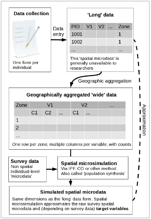
Figure 1. Schema of iterative proportional fitting (IPF) and combinatorial optimisation in the wider context of the availability of different data formats and spatial microsimulation.

Table 1: Usage characteristics of different terms for the IPF procedure, from the Scopus database. The percentages refer to the proportion of each search term used to refer to IPF in different subsets of the database: articles published since 2010 and mentioning "regional", respectively.
Search term	N. citations	Commonest subject area	% since 2010	% mentioning "regional"
Entropy maximisation	564	Engineering	30	9
"Iterative proportional fitting"	135	Mathematics	22	16
"RAS Algorithm"	25	Comp. science	24	24
"Iterative proportional scaling"	15	Mathematics	27	0
Matrix raking	12	Engineering	50	0
Biproportional estimation	12	Social sciences	17	33

1.12

Ambiguity in terminology surrounding the procedure has existed for a long time: when Michael Bacharach began using the term 'biproportional' late 1960s, he did so with the following caveat: "The 'biproportional' terminology is not introduced in what would certainly be a futile attempt to dislodge 'RAS', but to help to abstract the mathematical characteristics from the economic associations of the model" (Bacharach 1970). The original formulation of the procedure is generally ascribed to Deming and Stephan (1940), who presented an iterative procedure for solving the problem of how to modify internal cell counts of census data in 'wide' form, based on new marginal totals. Without repeating the rather involved mathematics of this discovery, it is worth quoting again from Bacharach (1970), who provided as clear a description as any of the procedure in plain English: "The method that Deming and Stephan suggested for computing a solution was to fit rows to the known row sums and columns to the known column sums by alternate [iterative] scalar multiplications of rows and columns of the base matrix" (1940, p. 4). The main purpose for revisiting and further developing the technique from Bacharach's perspective was to provide forecasts of the sectoral disaggregation of economic growth models. It was not until later (e.g. Clarke & Holm 1987) that the procedure was rediscovered for geographic research.

1.13

Thus IPF is a general purpose tool with multiple uses. In this paper we focus on its ability to disaggregate the geographically aggregated data typically provided by national statistical agencies to synthesise spatial microdata, as illustrated in Fig. 1.

1.14

In the physical sciences both data formats are common and the original long dataset is generally available. In the social sciences, by contrast, the long format is often unavailable due to the long history of confidentiality issues surrounding officially collected survey data. It is worth emphasising that National Census datasets | in which characteristics of every individual living in a state are recorded and which constitute some of the best datasets in social science – are usually only available in wide form. This poses major challenges to researchers in the sciences who are interested in intra-zone variability at the local level (Whitworth 2012; Lee 2009).

1.15

A related long-standing research problem especially prevalent in geography and regional science is the scale of analysis. There is often a trade-off between the quality and resolution of the data, which can result in a compromise between detail and accuracy of results. Often, researchers investigating spatial phenomena at many scales must use two datasets: one long non-spatial survey table where each row represents the characteristics of an individual – such as age, sex, employment status and income – and another wide, geographically aggregated dataset. IPF solves this problem when used in spatial microsimulation by proportional assignment of individuals to zones of which they are most representative.

IPF in spatial microsimulation

1.16

Spatial microsimulation tackles the aforementioned problems associated with the prevalent geographically aggregated wide data form by simulating the individuals within each administrative zone. The most detailed output of this process of spatial microsimulation is synthetic spatial microdata, a long table of individuals with associated attributes and weights for each zone (see Table 2 for a simple example). Because these individuals correspond to observations in the survey dataset, the spatial microdata generated in this way, of any size and complexity, can be stored with only three columns: person identification number (ID), zone and weight. Weights are critical to spatial microdata generated in this way, as they determine how representative each individual is of each zone. Synthetic spatial microdata taken from a single dataset can therefore be stored in a more compact way: a 'weight matrix' is a matrix with rows representing individuals and columns geographic zones. The internal cells reect how reective each individual is of each zone.

1.17

Representing the data in this form offers a number of advantages (Clarke & Holm 1987). These include:

• The ability to investigate intra-zone variation (variation within each zone can be analysed by subsetting a single area from the data frame).
• Cross-tabulations can be created for any combination of variables (e.g. age and employment status).
• The presentation of continuous variables such as income as real numbers, rather than as categorical count data, in which there is always data loss.
• The data is in a form that is ready to be passed into an individual-level model. For example individual behaviour could simulate traffic, migration or the geographical distribution of future demand for healthcare.

1.18

These benefits have not gone unnoticed by the spatial modelling community. Spatial microsimulation is now considered by some to be more than a methodology: it can be considered as a research field in its own right, with a growing body of literature, methods and software tools (Tanton & Edwards 2013). In tandem with these methodological developments, a growing number of applied studies is taking advantage of the possibilities opened up by spatial microdata. Published applications are diverse, ranging from health (e.g. Tomintz et al. 2008) to transport (e.g. Lovelace et al. 2014), and there are clearly many more domain areas in the social sciences where spatial microdata could be useful because human systems inherently operate on multiple levels, from individuals to nations.

1.19

IPF is used in the microsimulation literature to reweight individual-level data to fit a set of aggregate-level constraints. Its use was revived in the social sciences by Wong (1992), who advocated the technique's use for geographical applications and to help avoid various 'ecological fallacies' inherent to analysis of geographically aggregated counts (Openshaw 1984b).

1.20

A clear and concise definition is provided by Anderson (2013) in a Reference Guide (Tanton & Edwards 2013): "the method allocates all households from the sample survey to each small area and then, for each small area, reweights each household" (p. 53). Anderson (2013) also provides a simple explanation of the mathematics underlying the method. Issues to consider when performing IPF include selection of appropriate constraint variables, number of iterations and 'internal' and 'external' validation (Edwards & Clarke 2009; Pritchard & Miller 2012; Simpson & Tranmer 2005). It has been noted that IPF is an alternative to 'combinatorial optimisation' (CO) and 'generalised regression weighting' (GREGWT) (Hermes & Poulsen 2012). One issue with the IPF algorithm is that unless the fractional weights it generates intergerised, the results cannot be used as an input for agent-based models. Lovelace and Ballas (2013) provide an overview of methods for integerisation to overcome this problem. To further improve the utility of IPF there has been methodological work to convert the output into household units (Pritchard & Miller 2012).

1.21

In addition to IPF, other strategies for generating synthetic spatial microdata. These are described in recent overviews of the subject (Tanton & Edwards 2013; Ballas et al. 2013). The major (in terms of usage) alternatives are simulated annealing, an althorithm whose efficient implementation in Java is described by Harland (2013) and GREGWT, a deterministic approach resulting in fractional weights whose mathematics are described by Rahman (2009) (a recent open source implementation is available at https://gitlab.com/emunozh/mikrosim). However, it is not always clear which is most appropriate in different situations.

1.22

There has been work testing (Jiroušek & Přeučil 1995) and improving IPF model results (Teh & Welling 2003) but very little work systematically and transparently testing the algorithms underlying population synthesis (Harland et al. 2012). The research gap addressed in this paper is highlighted in the conclusions of a recent Reference Guide to spatial microsimulation: "It would be desirable if the spatial microsimulation community were able to continue to analyse which of the various reweighting/synthetic reconstruction techniques is most accurate – or to identify whether one approach is superior for some applications while another approach is to be preferred for other applications".

The IPF algorithm: a worked example

2.1

In most modelling texts there is a precedence of theory over application: the latter usually ows from the former (e.g. Batty 1976). As outlined in Section 1.1, however, the theory underlying IPF has been thoroughly demonstrated in research stemming back to the 1940s. Practical demonstrations are comparatively rare.

2.2

That is not to say that reproducibility is completely absent in the field. Simpson and Tranmer (2005) and Norman (1999) exemplify their work with code snippets from an implementation of IPF in the proprietary software SPSS and reference to an Excel macro that is available on request, respectively. Williamson (2007) also represents good practice, with a manual for running combinatorial optimisation algorithms described in previous work. Ballas et al. (2005) demonstrate IPF with a worked example to be calculated using mental arithmetic, but do not progress to illustrate how the examples are then implemented in computer code. This section builds on and extends this work, by first outlining an example that can be completed using mental arithmetic alone before illustrating its implementation in code. A comprehensive introduction to this topic is provided in a tutorial entitled "Introducing spatial microsimulation with R: a practical" (Lovelace 2014). This section builds on the tutorial by providing context and a higher level description of the process.

2.3

IPF is a simple statistical procedure "in which cell counts in a contingency table containing the sample observations are scaled to be consistent with various externally given population marginals" (McFadden et al. 2006). In other words, and in the context of spatial microsimulation, IPF produces maximum likelihood estimates for the frequency with which people appear in di_erent areas. The method is also known as 'matrix raking' or the RAS algorithm (Birkin & Clarke 1988; Simpson & Tranmer 2005; Kalantari et al. 2008; Jiroušek & Přeučil 1995), and has been described as one particular instance of a more general procedure of 'entropy maximisation' (Johnston & Pattie 1993; Blien & Graef 1998).

2.4

The mathematical properties of IPF have been described in several papers (Bishop et al. 1975; Fienberg 1970; Birkin & Clarke 1988). Illustrative examples of the procedure can be found in Saito (1992), Wong (1992) and Norman (1999). Wong (1992) investigated the reliability of IPF and evaluated the importance of different factors inuencing the its performance. Similar methodologies have since been employed by Mitchell et al. (2000), Williamson et al. (2002) and Ballas et al. (2005) to investigate a wide range of phenomena.

2.5

We begin with some hypothetical data. Table 2 describes a hypothetical microdataset comprising 5 individuals, who are defined by two constraint variables, age and sex. Table 3 contains aggregated data for a hypothetical area, as it might be downloaded from census dissemination portals such as Casweb.^[2] Table 4 illustrates this table in a different form, demonstrating the unknown links between age and sex. The job of the IPF algorithm is to establish estimates for the unknown cells, which are optimized to be consistent with the known row and column marginals.

Table 2: A hypothetical input microdata set (the original weights set to one). The bold value is used subsequently for illustrative purposes.
Individual	Sex	Age	Weight
1	Male	59	1
2	Male	54	1
3	Male	35	1
4	Female	73	1
5	Female	49	1

Table 3: Hypothetical small area constraints data (s).
Constraint ⇒	i		j
Category ⇒	i1	i2	j1	j2
Area ↓	Under-50	Over-50	Male	Female
1	8	4	6	6

Table 4: Small area constraints expressed as marginal totals, and the cell values to be estimated.
Marginal totals	j
	Age/sex	Male	Female	T
i	Under-50	?	?	8
	Over-50	?	?	4
	T	6	6	12

2.6

Table 5 presents the hypothetical microdata in aggregated form, that can be compared directly to Table 4. Note that the integer variable age has been converted into a categorical variable in this step, a key stage in geographical aggregation. Using these data it is possible to readjust the weights of the hypothetical individuals, so that their sum adds up to the totals given in Table 4 (12). In particular, the weights can be readjusted by multiplying them by the marginal totals, originally taken from Table 3 and then divided by the respective marginal total in 5. Because the total for each small-area constraint is 12, this must be done one constraint at a time. This is expressed, for a given area and a given constraint (i, age in this case) in Eq. (1).

Table 5: Aggregated results of the weighted microdata set (m(1)). Note, these values depend on the weights allocated in Table 2 and therefore change after each iteration.
Marginal totals	j
	Age/sex	Male	Female	T
i	Under-50	1	1	2
	Over-50	2	1	3
	T	3	2	5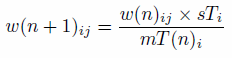

(1)

2.7

In Eq. (1), w(n + 1)_ij is the new weight for individuals with characteristics i (age, in this case), and j (sex), w(n)_ij is the original weight for individuals with these characteristics, sT_i is element marginal total of the small area constraint, s (Table 3) and mT(n)_i is the marginal total of category j of the aggregated results of the weighted microdata, m (Table 5). n represents the iteration number. Although the marginal totals of s are known, its cell values are unknown. Thus, IPF estimates the interaction (or cross-tabulation) between constraint variables. Follow the emboldened values in the Tables 2 to 6 to see how the new weight of individual 3 is calculated for the sex constraint. Table 6 illustrates the weights that result. Notice that the sum of the weights is equal to the total population, from the constraint variables.

Table 6: Reweighting the hypothetical microdataset in order to fit Table 3.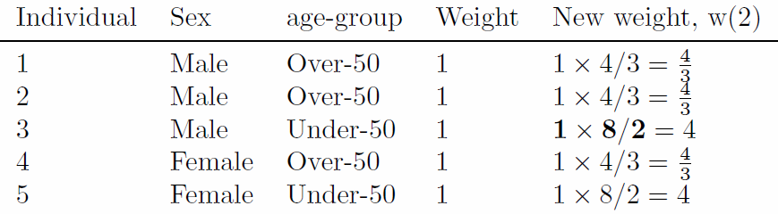

2.8

After the individual level data have been re-aggregated (Table 7), the next stage is to repeat Eq. (1) for the age constraint to generate a third set of weights, by replacing the i in sT_i and mT(n)_i with j and incrementing the value of n:

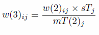
(2)

2.9

Apply Eq. (2) to the information above and that presented in Table 7 results in the following vector of new weights, for individuals 1 to 5:

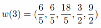
(3)

2.10

As before, the sum of the weights is equal to the population of the area (12). Notice also that after each iteration the fit between the marginal totals of m and s improves. The total absolute error (TAE, described in the next section) improves in m(1) to m(2) from 14 to 6 in Table 5 and Table 7 above. TAE for m(3) (not shown, but calculated by aggregating w(3)) improves even more, to 1.3. This number would eventually converge to 0 through subsequent iterations, as there are no 'empty cells' (Wong 1992) in the input microdataset, a defining feature of IPF (see Section 3.13 for more on the impact of empty cells).

Table 7: The aggregated results of the weighted microdata set after constraining for age (m(2)).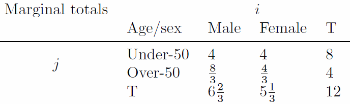

2.11

The above process, when applied to more categories (e.g. socio-economic class) and repeated iteratively until a satisfactory convergence occurs, results in a series of weighted microdatasets, one for each of the small areas being simulated. This allows for the estimation of variables whose values are not known at the local level (e.g. income) (Ballas et al. 2005). An issue with the results of IPF is that it results in non-integer weights: fractions of individuals appear in simulated areas. This is not ideal for certain applications, leading to the development of strategies to 'integerise' the fractional weights illustrated in Table 7. Methods for performing integerisation are discussed in Ballas et al. (2005), Pritchard and Miller (2012) and, most recently in Lovelace and Ballas (2013), who systematically benchmarked and compared different procedures. It was found that the probabilistic 'truncate, replicate, sample' (TRS) and 'proportional probabilities' methods – which use repeat sampling on the raw weights and non-repeat sampling (whereby a selected individual cannot be selected again) of the truncated weights, respectively – were most accurate. These methods are therefore used to test the impact of integerisation in this paper.

Evaluation techniques

3.1

To verify the integrity of any model, it is necessary to compare its outputs with empirical observations or prior expectations gleaned from theory. The same principles apply to spatial microsimulation, which can be evaluated using both internal and external validation methods (Edwards & Clarke 2009). Internal validation is the process whereby the aggregate-level outputs of spatial microsimulation are compared with the input constraint variables. It is important to think carefully about evaluation metrics because results can vary depending on the measure used (Voas & Williamson 2001).

3.2

Internal validation typically tackles such issues as "do the simulated populations in each area microdata match the total populations implied by the constraint variables?" and "what is the level of correspondence between the cell values of different attributes in the aggregate input data and the aggregated results of spatial microsimulation?" A related concept from the agent based modelling literature is verification, which asks the more general question, "does the model do what we think it is supposed to do?" (Ormerod & Rosewell 2009, p. 131) External validation is the process whereby the variables that are being estimated are compared to data from another source, external to the estimation process, so the output dataset is compared with another known dataset for those variables. Both validation techniques are important in modelling exercises for reproducibility and to ensure critical advice is not made based on coding errors (Ormerod & Rosewel 2009).

3.3

Typically only aggregate-level datasets are available, so researchers are usually compelled to focus internal validation as the measure model performance. Following the literature, we also measure performance in terms of aggregate-level fit, in addition to computational speed. A concern with such a focus on aggregate-level fit, prevalent in the literature, is that it can shift attention away from alternative measures of performance. Provided with real spatial microdata, researchers could use individual-level distributions of continuous variables and comparison of joint-distributions of cross-tabulated categorical variables between input and output datasets as additional measures of performance. However one could argue that the presence of such detailed datasets removes the need for spatial microsimulation (Lee 2009). Real spatial microdata, where available, offer an important opportunity for the evaluation of spatial microsimulation techniques. However, individual-level external validation is outside the scope of this study.

3.4

For dynamic microsimulation scenarios, calculating the sampling variance (the variance in a certain statistic, usually the mean, across multiple samples) across multiple model runs is recommended to test if differences between different scenarios are statistically significant (Goedemé et al. 2013). In static spatial microsimulation, sub-sampling from the individual level dataset or running stochastic processes many times are ways to generate such statistics for tests of significance. Yet these statistics will only apply to a small part of the modelling process and are unlikely to relate to the validity of the process overall (Lovelace & Ballas 2013).

3.5

This section briey outlines the evaluation techniques used in this study for internal validation of static spatial microsimulation models. The options for external validation are heavily context dependent so should be decided on a case-by-case basis. External validation is thus mentioned in the discussion, with a focus on general principles rather than specific advice. The three quantitative methods used in this study (and the visual method of scatter plots) are presented in ascending order of complexity and roughly descending order of frequency of use, ranging from the coefficient of determination (R²) through total and standardised absolute error (TAE and SAE, respectively) to root mean squared error (RMSE). This latter option is our preferred metric, as described below.

3.6

Before these methods are described, it is worth stating that the purpose is not to find the 'best' evaluation metric: each has advantages and disadvantages, the importance of which will vary depending on the nature of the research. The use of a variety of techniques in this paper is of interest in itself. The high degree of correspondence between them (presented in Section 5), suggests that researchers need only to present one or two metrics (but should try more, for corroboration) to establish relative levels of goodness of fit between different model configurations.

3.7

The problem of internal validation (described as 'evaluating model fit') was tackled in detail by Voas and Williamson (2001). The Chi-squared statistic, Z-scores, absolute error and entropy-based methods were tested, with no clear 'winner' other than the advocacy of methods that are robust, fast and easy to understand (standardized absolute error measures match these criteria well). The selection of evaluation methods is determined by the nature of available data: "Precisely because a full set of raw census data is not available to us, we are obliged to evaluate our simulated populations by comparing a number of aggregated tables derived from the synthetic data set with published census small-area statistics" (Voas & Williamson 2001, p. 178). A remaining issue is that the results of many evaluation metrics vary depending on the areal units used, hence advocacy of 'scale free' metrics (Malleson & Birkin 2012) .

Scatter plots

3.8

A scatter plot of cell counts for each category for the original and simulated variables is a basic but very useful preliminary diagnostic tool in spatial microsimulation (Ballas et al. 2005; Edwards & Clarke 2009). In addition, marking the points, depending on the variable and category which they represent, can help identify which variables are particularly problematic, aiding the process of improving faulty code (sometimes referred to as 'debugging'). In these scatter plots each data point represents a single zone-category combination (e.g. 16–25 year old female in zone 001), with the x axis value corresponding to the number of individuals of that description in the input constraint table. The y value corresponds to the aggregated count of individuals in the same category in the aggregated (wide) representation of the spatial microdata output from the model. This stage can be undertaken either before or after integerisation (more on this below). As is typical in such circumstances, the closer the points to the 1:1 (45 degree, assuming the axes have the same scale) line, the better the fit.

The coefficient of determination

3.9

The coefficient of determination (henceforth R²) is the square of the Pearson correlation coefficient for describing the extent to which one continuous variable explains another. R² is a quantitative indicator of how much deviation there is from this ideal 1:1 line. It varies from 0 to 1, and in this context reveals how closely the simulated values fit the actual (census) data. An R² value of 1 represents a perfect fit; an R² value close to zero suggests no correspondence between then constraints and simulated outputs (i.e. that the model has failed). We would expect to see R² values approaching 1 for internal validation (the constraint) and a strong positive correlation between target variables that have been estimated and external datasets (e.g. income). A major limitation of R² is that it takes no account of additive or proportional differences between estimated and observed values, meaning that it ignores systematic bias (see Legates & McCabe 1999 for detail). This limitation is less relevant for spatial microsimulation results because they are generally population-constrained.

Total Absolute and Standardized Error (TAE and SAE)

3.10

Total absolute error (TAE) is the sum of the absolute (always positive) discrepancies between the simulated and known population in each cell of the geographically aggregated (wide format) results. The standardised absolute error (SAE) is simply TAE divided by the total population (Voas & Williamson 2001). TAE provides no level of significance, so thresholds are used. Clarke & Madden (2001) used an error threshold of 80 per cent of the areas with less than 20 per cent error (SAE <0.20); an error threshold of 10% (SAE <0.1) can also been used Smith et al. (2007). Due to its widespread use, simplicity and scale-free nature, SAE is often preferred.

The modified Z-score

3.11

The Z-statistic is a commonly used measure, reporting the number of standard deviations a value is from the mean. In this work we report zm, a modified version to the Z-score metric that is robust to very small expected cell values (Williamson et al. 1998). Z-scores apply to individual cells (for a single constraint in a single area). and also provide a global statistic on model fit (Zm), defined as the sum of all zm² values (Voas & Williamson 2001). The measure of fit has the advantage of taking into account absolute, rather than just relative, differences between simulated and observed cell count:

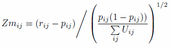
(4)

where

3.12

To use the modified Z-statistic as a measure of overall model fit, one simply sums the squares of zm to calculate Zm². This measure can handle observed cell counts below 5, which chi-squared tests cannot (Voas & Williamson 2001).

Proportion of values deviating from expectations E > 5%

3.13

The proportion of values which fall beyond 5% of the actual values is a simple metric of the quality of the fit. It focusses on the proportion of values which are close to expected, rather than the overall fit, so is robust to outliers. The E > 5% metric implies that getting a perfect fit is not the aim, and penalises relationships that have a large number of moderate outliers, rather than a few very large outliers. The precise definition of 'outlier' is somewhat arbitrary (one could just as well use 1%).

Root mean square error

3.14

Root mean square error (RMSE) and to a lesser extent mean absolute error (MAE) have been frequently used in both social and physical sciences as a metric of model fit (Legates & McCabe 1999). Like SAE, the RMSE takes the discrepancies between the simulated and known values, squares these and divides the sum by the total number of observations (areas in our case), after which the root is taken. The MAE basically does the same without the square and root procedure. The former has the benefit of being widely used and understood, but is inuenced by the mean value in each zone. Recent research in climate model evaluation suggests that the lesser known but simpler MAE metric is preferable to RMSE in many ways (Willmott & Matsuura 2005). We use the RMSE error in the final results as this is a widely understood and applied method with a proven track record in the social sciences. The relationship between these different goodness-of-fit measures was tested, the results of which can be seen towards the end of Section 5.

Input data

4.1

The size and complexity of input data inuence the results of spatial microsimulation models. Especially important are the number of constraint variables and categories. We wanted to test the method under a range of conditions. Therefore, three unrelated scenarios, each with their own input datasets were used. These are referred to as 'simple', 'small-area' and 'Sheffield'. Each consists of a set of aggregate constraints and corresponding individual-level survey tables. To ensure reproducibility, all the input data (and code) used to generate the results reported in the paper are available online on the code-sharing site GitHub.^[3] An introductory tutorial explains the process of loading and 'cleaning' input data (Lovelace 2014). This tutorial also introduces the basic code used to create and modify the weight matrices with reference to the 'simple' example described below.

4.2

The simplest scenario consists of 6 zones which must be populated by the data presented in the previous section (see Table 2). This scenario is purely hypothetical and is used to represent the IPF procedure and the tests in the simplest possible terms. Its small size allows the entirety of the input data to be viewed in a couple of tables (see Table 2 and Table 8, the first row of which is used to exemplify the method). As wit hall data used in this paper, these tables can be viewed and downloaded online.

Table 8: Geographically aggregated constraint variables for the simple scenario.
	Age constraint		Sex constraint
Zone	16–49	50+	m	f
1	8	4	6	6
2	2	8	4	6
3	7	4	3	8
4	5	4	7	2
5	7	3	6	4
6	5	3	2	6

4.3

The next smallest input dataset, and the most commonly used scenario in the paper, is 'small-area'. The area constraints consist of 24 Output Areas (the smallest administrative unit in the UK), with an average adult population of 184. Three constraint files describe the number of people (number of households for tenancy) in each category for the following variables:

• hours worked (see 'input-data/small-area-eg/hrs-worked.csv', which consists of 7 categories from '1–5' to '49+' hours per week)
• marital status (see 'marital-status.csv', containing 5 categories)
• tenancy type ('tenancy.csv', containing 7 categories).

4.4

The individual-level table that complements these geographically aggregated count constraints for the 'small area' example is taken from Understanding Society wave 1. These have been randomised to ensure anonymity but they are still roughly representative of real data. The table consists of 1768 rows of data and is stored in R's own space-efficient file-type (see "ind.RData", which must be opened in R). This and all other data files are contained within the 'input-data' folder of the online repository (see the 'input-data' sub-directory of the Supplementary Information).

4.5

The largest example dataset is 'Sheffield', which represents geographically aggregated from the UK city of the same name, provided by the 2001 Census. The constraint variables used in the baseline version of this model can be seen in the folder 'input-data/sheffield' of the Supplementary Information. They are:

• A cross-tabulation of 12 age/sex categories
• Mode of travel to work (11 variables)
• Distance travelled to work(8 variables)
• Socio-economic group (9 variables)

4.6

As with 'small-area', the individual-level dataset associated with this example is a scrambled and anonymised sample from the Understanding Society. In addition to those listed above at the aggregate level, 'input-data/sheffield/ind.RData' contains columns on whether their home location is urban/rural (variable 'urb'), employment status ('stat') and home region ('GOR').

Method: model experiments

Baseline conditions

5.1

Using the three different datasets, the effects of five model settings were assessed: number of constraints and iterations; initial weights; empty cell procedures; and integerisation. In order to perform a wide range of experiments, in which only one factor is altered at a time, baseline scenarios were created. These are model runs with sensible defaults and act as reference points against which alternative runs are compared. The baseline scenarios consist of 3 iterations. In the 'simple' scenario (with 2 constraints), there are 6 constraint-iteration permutations. The fit improves with each step. The exception is p5, which reaches zero in the second iteration. pcor continues to improve however, even though the printed value, to 6 decimal places, is indistinguishable from 1 after two complete iterations.

5.2

The main characteristics of the baseline model for each scenario are presented in Table 9. The meaning of the row names of Table 9 should become clear throughout this section.

Table 9: Characteristics of the baseline model run for each scenario.
Scenario	Simple	Small area	Sheffield
N. constraints	2	3	4
N. zones	6	24	71
Av. individuals/zone	10	184	3225
Microdataset size	5	1768	4933
Average weight	1.3	0.1	0.65
% empty cells	0%	21%	85%

Constraints and iterations

5.3

The number of constraints refers to the number of separate categorical variables (e.g. age bands, income bands). The number of iterations is the number of times IPF adjusts the weights according to all available constraints. Both are known to be important determinants of the final output, but there has been little work to identify the optimal number of either variable. Norman (1999) suggested including the "maximum amount of information in the constraints", implying that more is better. Harland et al. (2012), by contrast, notes that the weight matrix can become overly sparse if the model is over-constrained. Regarding the number of iterations, there is no clear consensus on a suitable number, creating a clear need for testing in this area.

5.4

Number of constraints and iterations were the simplest model experiments. These required altering the number of iterations or rearranging of the order in which constraints were applied. 1, 3 and 10 iterations were tested and all combinations of constraint orders were tested.^[4]"

5.5

To alter the number of iterations used in each model, one simply changes the number in the following line of code (the default is 3):

num.its <- 3

The code for running the constraints in a different order is saved in 'etsim-reordered.R'. In this script file, the order in which constraints ran was systematically altered. The order with the greatest impact on the results for each example is reported in Table 11.

5.6

In real-world applications, there is generally a 'more the merrier' attitude towards additional constraints. However, Harland et al. (2012) warn of the issues associated with over-fitting microsimulation models with too many constraints. To test the impact of additional constraints we added a new constraint to the small-area and Sheffield examples. A cross-tabulated age/sex constraint was added for the small-area example; a binary urban/rural constraint was added for the Sheffield example. In both cases the scripts that implement IPF with these additional constraint variables are denoted by the text string "extra-con", short for "extra constraint" and include 'etsim-extra-con.R' and 'categorise-extra-con.R'.

Initial weights

5.7

The mathematics of IPF show that it converges towards a single solution of 'maximum likelihood' (Jiroušek & Přeučil 1995) yet initial weights can impact the results of the model result when a finite number of iterations is used. The persistence of the impact of initial weights has received little attention. The impact of initial weights was tested in two ways: first, the impact of changing a sample of one or more initial weight values by a set amount was explored. Second, the impact of gradually increasing the size of the initial weights was tested, by running the same model experiment several times, but with incrementally larger initial weights applied to a pre-determined set of individuals.

5.8

In the simplest scenario, the initial weight of a single individual was altered repeatedly, in a controlled manner. To observe the impacts of altering the weights in this way the usual tests of model fit were conducted. In addition, the capacity of initial weights to inuence an individual's final weight/probability of selection was tested by tracing its weight into the future after each successive constraint and iteration. This enabled plotting original vs simulated weights under a range of conditions (Section 5.18).

5.9

In the final results, extreme cases of setting initial weights are reported: setting a 10% sample to 100 and 1000 times the default initial weight of 1. In the baseline scenario there are only 3 iterations, allowing the impacts of the initial weights to linger. This inuence was found to continue to drop, tending towards zero inuence after 10 iterations even in the extreme examples.

Empty cells

5.10

Empty cells refer to combinations of individual-level attributes that are not represented by any single individual in the survey input data. An example of this would be if no female in the 16 to 49 year age bracket were present in Table 2. Formalising the definition, survey dataset that contains empty cells may be said to be incomplete; a survey dataset with no empty cells is complete. Wong (1992) was the first to describe the problem of empty cells in the context of spatial microsimulation, and observed that the procedure did not converge if there were too many in the input microdata. However, no methods for identifying their presence were discussed, motivating the exploration of empty cells in this paper.

5.11

No method for identifying whether or not empty cells exist in the individual-level dataset for spatial microsimulation has been previously published to the authors' knowledge. We therefore start from first principles. The number of different constraint variable permutations (Nperm) is defined by Eq. (5), where n:cons is the total number of constraints and n:cat_i is the number of categories within constraint i:

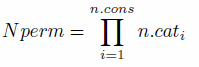
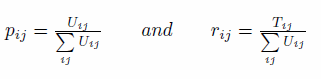
(5)

5.12

To exemplify this equation, the number of permutations of constraints in the 'simple' example is 4: 2 categories in the sex variables multiplied by 2 categories in the age variable. Clearly, Nperm depends on how continuous variables are binned, the number of constraints and diversity within each constraint. Once we know the number of unique individuals (in terms of the constraint variables) in the survey (Nuniq), the test to check a dataset for empty cells is straightforward, based on Eq. (5):

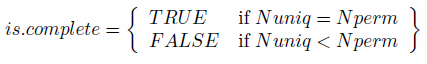
(6)

5.13

Once the presence of empty cells is determined in the baseline scenarios, the next stage is to identify which individuals are missing from the individual-level input dataset (Ind) – the combination of attributes that no individual in Ind has. To do this, we created an algorithm to generate the complete input dataset (Ind:complete). The 'missing' individuals, needed to be added to make Ind complete can be de_ned in terms of set theory (Goldrei 1996) by Eq. (7):

(7)

5.14

This means simply that the missing cells are defined as individuals with constraint categories that are present in the complete dataset but absent from the input data. The theory to test for and identify empty cells described above is straightforward to implement in practice with R, using the commands unique and %in% respectively (see the 'empty-cells.R' script in the 'model' folder of the code repository).

5.15

To test the impact of empty cells on model results, an additional empty cell was added to the input dataset in each example. In the 'simple' scenario, this simply involves removing a single individual from the input data, which equates to deleting a single line of code (see 'empty-cells.R' in the 'simple' folder to see this). Experiments in which empty cells were removed through the addition of individuals with attributes defined by Eq. (7) were also conducted, and the model fit was compared with the baseline scenarios. The baseline scenarios were run using these modified inputs.

Integerisation

5.16

Integerisation is the process of converting the fractional weights produced by IPF into whole numbers. It is necessary for some applications, including the analysis of intra-zone variability and statistical analyses of intra-zone variation such as the generation of Gini indices of income for each zone.

5.17

A number of methods for integerisation have been developed, including deterministic and probabilistic approaches (Ballas et al. 2005). We used modified R implementations of two probabilistic methods – 'truncate replicate sample' (TRS) and 'proportional probabilities' – reported in Lovelace and Ballas (2013) and the Supplementary Information associated with this paper (Lovelace 2013), as these were found to perform better in terms of final population counts and accuracy than the deterministic approaches.

Computational efficiency

5.18

The code used for the model runs used throughout this paper is based on that provided in the Supplementary Information of Lovelace and Ballas (2013). This implementation was written purely in R, a vector based language, and contains many 'for' loops, which are generally best avoided for speed-critical applications. R was not designed for speed, but has interfaces to lower level languages (Wickham 2014a). Another advantage of R from the perspective of synthetic populations is that it has an interface to NetLogo, a framework for agent-based modelling (Thiele 2014). One potential use of the IPF methods outlined in this paper is to generate realistic populations to be used for model experiments in other languages (see Thiele et al. 2014).

5.19

To increase the computational efficiency of R, experiments were conducted using the ipfp package, a C implementation of IPF (Blocker 2013).

5.20

For each scenario in the Supplementary Information, there is a file titled 'etsim-ipfp.R', which performs the same steps as the baseline 'etsim.R' model run, but using the ipfp() function of the ipfp package. The results of these experiments for different scenarios and different numbers of iterations are presented in Section 5.6.

Results

Baseline results

6.1

After only 3 complete iterations under the baseline conditions, the final weights in each scenario converged towards a final result. The baseline 'Sheffield' scenario consists of the same basic set-up, but with 4 constraints. As before, the results show convergence towards better model fit, although the fit did not always improve from one constraint to the next.

Constraints and iterations

6.2

As shown in Fig. 2, fit improved with each iteration. This improvement generally happened for each constraint and always from one iteration to the next. Through the course of the first iteration in the 'simple' scenario, for example, R² improved from 0.67 to 0.9981. There is a clear tendency for the rate of improvement in model fit to drop with subsequent computation after the first iteration: at the end of iteration 2 in the simple scenarios, R² had improved to 0.999978.

6.3

The results for the first 6 constraint-iteration permutations of this baseline scenario are illustrated in Fig. 3 and in the online 'measures' table. These results show that IPF successfully took the simulated cell counts in-line with the census after each constraint and that the fit improves with each iteration (only two iterations are shown here, as the fit improves very little beyond two).

6.4

Rapid reductions in the accuracy improvement from additional computation were observed in each scenario, as illustrated by the rapid alignment of zone/constraints to the 1:1 line in Fig. 3. After four iterations, in the 'simple' scenarios, the fit is near perfect, with an R² value indistinguishable from one to 7 decimal places. The decay in the rate of improvement with additional iterations is super-exponential.

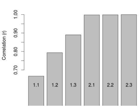
Figure 2. Improvement in goodness of fit with additional constraints and iterations, as illustrated by R2 values.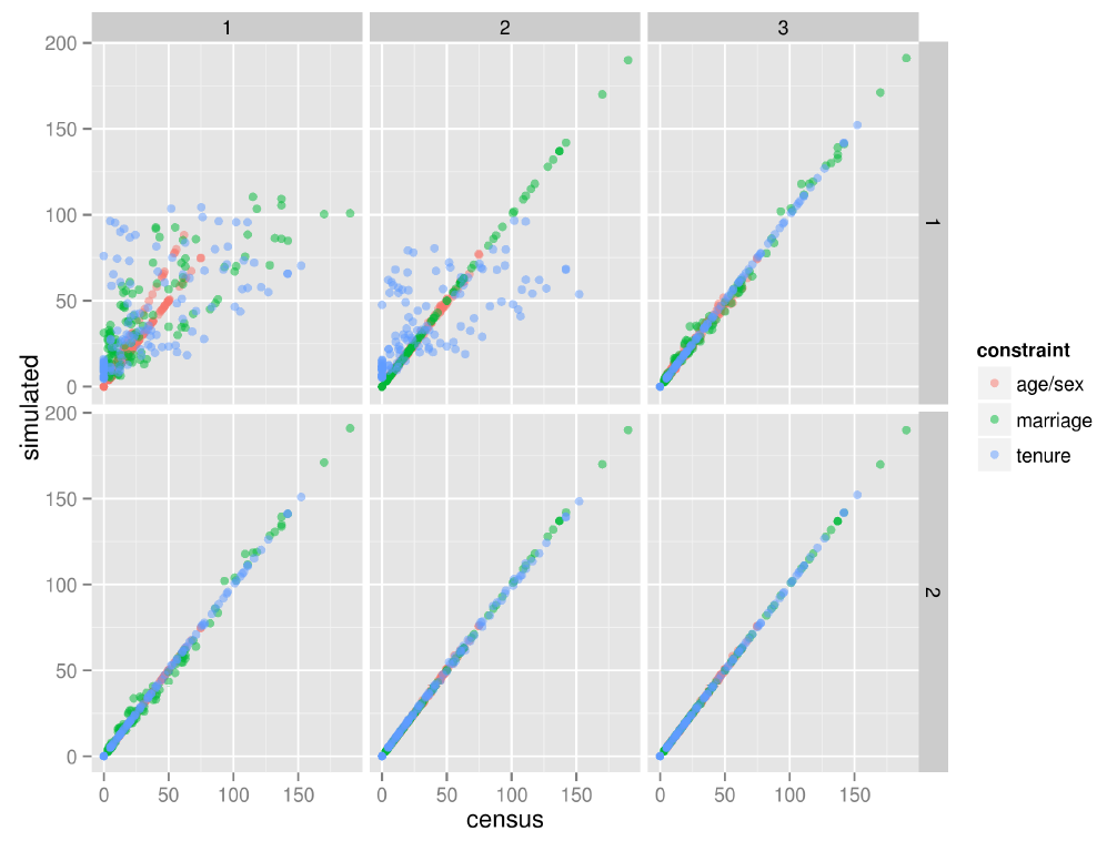

Figure 3. IPF in action: simulated vs census zone counts for the small-area baseline scenario after each constraint (columns) and iteration (rows).

6.5

It was found that additional constraints had a detrimental impact on overall model fit. The impact was clearly heavily inuenced by the nature of the new constraint, however, meaning we cannot draw strong conclusions from this result. In any case, the results show that additional constraints have a negative impact on model fit.

6.6

Interestingly, the addition of the urban/rural constraint variable in the Sheffield example had the most dramatic negative impact of all model experiments. This is probably because this is a binary variable even at the aggregate level, whereby all residents are classified as 'rural' or 'urban'. Only 17% (830 out of 933) of the respondents in the individual-level survey are classified as rural dwellers, explaining why fit dropped most dramatically for rural areas.

67.7

The order of constraints was found to have a strong impact on the overall model fit. It was found that placing constraints with more categories towards the end of the iterative fitting process had the most detrimental effect. The impact of placing the age/sex constraint last in the 'Sheffield' example, which had 12 variables, had the most damaging impact on model fit. This was due to the relative complexity of of this constraint and its lack of correlation with the other constraints in the individual-level dataset. We note that selection of constraint order introduces a degree of subjectivity into the results of IPF: the researcher is unlikely to know at the outset which constraint variable will have the most detrimental impact on model fit (and therefore which should not be used last).

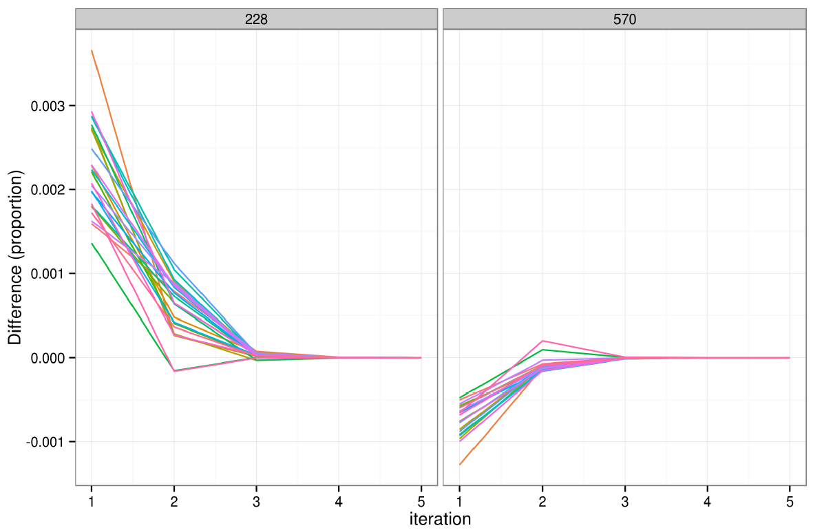
Figure 4. The impact of changing the initial weight of individual 228 on the simulated weights of two individuals after 5 iterations. Each of the 24 coloured lines represents a single zone.

Initial weights

6.8

It was found that initial weights had little impact on the overall simulation. Taking the simplest case, a random individual (id = 228) was selected from the 'small area' data and his/her initial weight was set to 2 (instead of the default of 1). The impact of this change on the individual's simulated weight decayed rapidly, tending to zero after only 5 iterations in the small-area scenario. It was found that altered initial weights affect the simulated weights of all other individuals; this is illustrated in Fig. 4, which shows the impact on individual 228 and a randomly selected individual whose initial weight was not altered, for all areas.

6.9

Fig. 4 shows that changing initial weights for individuals has a limited impact on the results that tends to zero from one iteration to the next. After iteration one the impact of a 100% increase in the initial weight of individual 228 had reduced to 0.3%; after 3 iterations the impact was negligible. The same pattern can be observed in the control individual 570, although the impact is smaller and in the reverse direction. The same pattern can be observed for other individuals, by altering the 'analysis.min'.

6.10

To analyse the impacts of changing the initial weights of multiple individuals, the same experiment was conducted, but this time the initial weights were applied to the first five individuals. The results are illustrated in Fig. 5, which shows the relationship between initial and final weights for the first two individuals and another two individuals (randomly selected to show the impact of altering weights on other individual weights).

6.11

Fig. 5 shows that the vast majority of the impact of altered starting weights occurs in iteration-constraint combinations 1.1 and 1.2, before a complete iteration has even occurred. After that, the initial weights continue to have an inuence, of a magnitude that cannot be seen. For individual 1, the impact of a 53% difference in initial weights (from 0.7 to 1.5) shrinks to 2.0% by iteration 1.3 and to 1.1% by iteration 2.3.

6.12

These results suggest that initial weights have a limited impact on the results of IPF, that declines rapidly with each iteration.

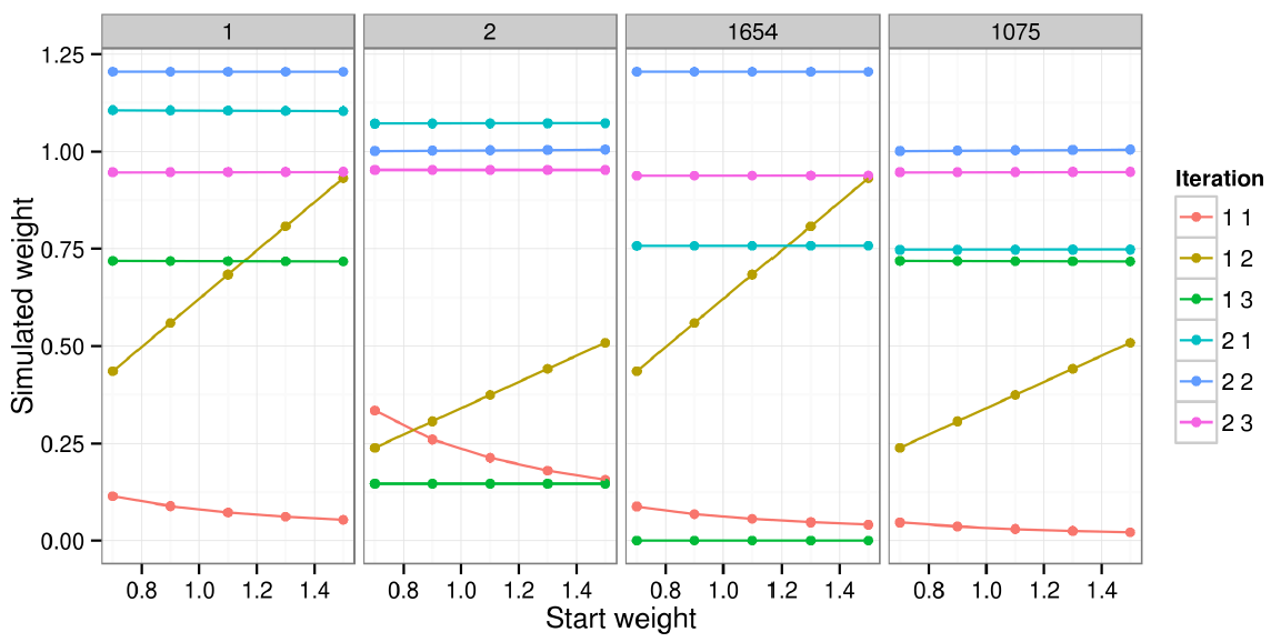
Figure 5. Initial vs simulated weight of four individuals for a single area (zone 1).

Empty cells

6.13

There were found to be 62 and 8,105 empty cells in the 'small-area' and 'Sheffield' baseline scenarios, respectively. Only the smallest input dataset was complete. Due to the multiplying effect of more variables (Eq. (5)), Nperm was found to be much larger in the complex models, with values rising from 4 to 300 and 9504 for the increasingly complex test examples.

6.14

As expected, it was found that adding additional empty cells resulted in worse model fit, but only slightly worse fit if few empty cells (one additional empty cell to 10% non-empty cells) were added. The addition of new rows of data with attributes corresponding to the empty cells to the input dataset allowed the 'small-area' and 'Sheffield' models to be re-run without empty cells. This resulted in substantial improvements in model fit that became relatively more important with each iteration: model runs with large numbers of empty cells reached minimum error values quickly, beyond which there was no improvement.

Integerisation

6.15

After passing the final weights through the integerisation algorithms mentioned in Section 4.5, the weight matrices were of identical dimension and total population as before. It was found that, compared with the baseline scenarios, that integerisation had a negative impact on model fit. For the 'simple' and 'small area' scenarios, the impact of integerisation was proportionally large, greater than the impact of any other changes. For the more complex Sheffield example, by contrast, the impact was moderate, increasing RMSE by around 20%.

Computational efficiency

6.16

The times taken to perform IPF in the original R code and the new low-level C implementation are compared in Table 10. This shows that running the repetitive part of the modelling in a low-level language can have substantial speed benefits – more than 10 fold improvements were found for all but the simplest model runs with the fewest iterations. Table 10 shows that the computational efficiency benefits of running IPF in C are not linear: the relative speed improvements increase with the both the number of iterations and the size of the input datasets.

6.17

This suggests two things:

• Other parts of the R code used in both the 'pure R' and C implementations via ipfp could be optimised for speed improvements.
• Greater speed improvements could be seen with larger and more complex model runs.

Summary of results

6.18

The impact of each model experiment on each of the three scenarios is summarised in Table 11. It is notable that the variable with the greatest impact on model fit varied from one scenario to the next, implying that the optimisation of IPF for spatial microsimulation is context-specific. Changes that had the greatest positive impact on model fit were additional iterations for the simpler scenarios and the removal of empty cells from the input microdata for the more complex 'Sheffield' scenario.

6.19

Likewise, the greatest negative impact on model fit for the 'small area' example was due to integerisation. For 'Sheffield', the addition of the unusual urban/rural binary variable had the greatest negative impact on model fit. The use of only one complete iteration instead of 3 or more had more damaging impacts on the larger and more complicated examples.

Table 10: Time taken for different spatial microsimulation models to run in microseconds, comparing R and C implementations code. 3 (left hand columns) and 10 (right hand columns) iterations were tested for each. 'Improvement' represents the relative speed improvement of the C implementation, via the ipfp package.
	3 iterations			10 iterations
Scenario	R code	C code (ipfp)	Improvement	R code	C code (ipfp)	Improvement
Simple	73	8	9.1	231	8	28.9
Small-area	3548	204	17.4	10760	288	37.4
Sheffield	44051	1965	22.4	135633	2650	51.2

6.20

Substantial improvements in execution speed have been demonstrated using a lower-level implementation of the IPF algorithm than has been used in previous research. If computational efficiency continues to increase, the code could run 100 times faster than current implementations on larger datasets (see Table 10).

Table 11: Summary results of root mean square error (RMSE) between simulated and constraint data.
Test scenario	Simple	Small area	Sheffield
Baseline	0.0001	0.018	25.5
Constraints and iterations
1 iteration	0.221	1.91	78.2
5 iterations	<0.000001	0.00001	20.9
10 iterations	<0.000001	0.000002	13.8
Reordered constraints	0.0001	0.018	14.5
Extra constraint	—	1.57	283
Initial weights
10% sample set to 10	0.0001	0.034	25.5
10% sample set to 1000	0.0001	0.998	25.5
Empty cells
1 additional empty cell	0.852	0.018	25.5
10% additional empty cells	—	0.050	25.6
No empty cells	—	0.005	1.24
Integerisation
TRS integerisation	0.577	3.68	29.9
Proportional probabilities	1.29	3.91	30.0

6.21

The results presented in Table 11 were robust to the type of measure. We calculated values for the six goodness of fit metrics described in Section 3 and illustrated in Fig. 6 for each of the three example datasets. The results after 10 iterations of 'baseline' scenario are saved in table files titled 'measures.csv' in each of the model folders. The results for each metric in the Sheffield model, for example, can be found in 'models/sheffield/measures.csv'. The calculation, storage and formatting of this array of results is performed by the script 'analysis.R' in the models folder.

6.22

Overall it was found that there was very good agreement between the different measures of goodness-of-fit. Despite often being seen as crude, the r measure of correlation was found to be very closely related to the other measures. Unsurprisingly, the percentage of error metric ('E5' in Fig. 6) fitted worse with the others, because this is a highly non-linear measure that rapidly tends to 0 even when there is still a large amount of error.

6.23

The conclusion we draw from this is that although the absolute goodness-of-fit varies from one measure to the next, the more important relative fit of different scenarios remains unchanged. The choice of measure becomes more important when we want to compare the performance of different models which vary in terms of their total population. To test this we looked at the variability between different measures between each scenario, the results of which are shown in table 12. It is clear that r, SAE and E5 metrics have the advantage of providing a degree of cross-comparability between models of different sizes. TAE, RMSE and the sum of Z – squared scores, by contrast, are highly dependent on the total population.

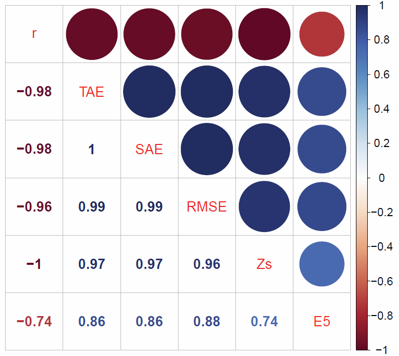
Figure 6. Correlation matrix comparing 6 goodness-of-fit measure for internal validation. The numbers to the bottom-left of the diagonal line represent Pearson's r, the correlation between the different measures. The circles represent the same information in graphical form. The abbreviation are as follows. r: Pearson's coefficient of correlation; TAE: Total Absolute Error; SAE: Standardised Absolute Error; Zs: Z-score; E5: Errors greater than 5% of the observed value.

Table 12: Summary statistics for the 6 goodness of _t measures for each iteration of each 'baseline' scenario.
Model (mean)	r	TAE	SAE	RMSE	Zs	E5
Simple	0.942	4.304	0.036	0.287	2.3640e+00	0.132
Small-area	0.964	968.934	0.073	4.195	1.1936e+07	0.160
Sheffield	0.972	89531.053	0.098	68.703	6.8430e+04	0.355
Model (SD)
Simple	0.138	8.762	0.073	0.584	5.6490e+00	0.215
Small-area	0.074	1734.436	0.131	7.224	2.3784e+07	0.204
Sheffield	0.046	89626.742	0.098	61.599	1.1313e+05	0.206

Conclusions

7.1

In this paper we have systematically reviewed and tested modifications to the implementation of the IPF algorithm for spatial microsimulation – i.e. the creation of spatial microdata. This is the first time to our knowledge that such tests have been performed in a consistent and reproducible manner, that will allow others to cross-check the results and facilitate further model testing. The model experiments conducted involved changing one of the following variables at a time:

• The order and number of constraints and number of iterations.
• Modification of initial weights.
• Addition and removal of 'empty cells'.
• Integerisation of the fractional weights using a couple of probabilistic methods – 'TRS' and 'proportional probabilities'.
• The language in which the main IPF algorithm is undertaken, from R to C via the ipfp package.

7.2

In every case, the direction of change was as expected, confirming prior expectations about the inuence of model set-up on performance. The finding that the initial weights have very little inuence on the results, particularly after multiple iterations of IPF, is new and relevant to the spatial microsimulation community. This finding all but precludes the modification of initial weights as a method for altering IPF's performance and suggests that research time would be best focused on other variables, notably empty cells.

7.3

A new contribution of this paper is its analysis of empty cells – individuals absent in the individual-level dataset but implied by the geographically aggregated constraints. The methods presented in Section 5.4 should enable others to identify empty cells in their input datasets and use this knowledge to explain model fit or to identify synthetic individuals to add. This is the first time, to our knowledge, that empty cells have been shown to have large adverse effect on model fit compared with other variables in model design.

7.4

The removal of empty cells greatly improved fit, especially for complex scenarios. This straightforward change had the single greatest positive impact on the results, leading to the conclusion that removing empty cells can substantially enhance the performance of spatial microsimulation models, especially those with many constraint variables and relatively small input input datasets. On the other hand, a potential downside of removing empty cells is that it involves adding fictitious new individuals to the input microdata. This could potentially cause problems if the purpose of spatial microsimulation is small area estimation, where the value of target variables (e.g. income) must be set. Another potential problem caused by removal of empty cells that must be avoided is the creation of impossible combinations of variables such as car drivers under the age of 16.

7.5

A useful practical finding is that IPF implemented using the ipfp package yields execution much faster than the R code described in Lovelace (2013). The speed benefit of this low-level implementation rose with additional iterations and model complexity, suggesting that the method of implementation may be more inuential than the number of iterations. Regarding the optimal number of iterations, there is no magic number identified in this research. However, it is clear that the marginal benefits of additional iterations decline rapidly: we conclude that 10 iterations should be sufficient for complete convergence in most cases.

7.6

Many opportunities for further research emerge from this paper on the specific topic of IPF and in relation to the field of spatial microsimulation more generally.

7.7

Questions raised relating to IPF include:

• What are the impacts of constraining by additional variables affecting the performance of IPF?
• What are the interactions between different variables – e.g. what is the combined impact of altering the number of empty cells and number of iterations simultaneously?
• Can change in one variable reduce the need for change in another?
• What are the opportunities for further improvements in computational efficiency of the code?
• How does IPF respond to unusual constraints, such as cross-tabulated contingency tables with shared variables (e.g. age/sex and age/class)?
• How are the results of IPF (and other reweighting methods) affected by correlations between the individual-level variables?

7.8

There is clearly a need for further testing in the area of spatial microsimulation overall, beyond the specific example of IPF in R used here. The generation of synthetic populations allocated to specific geographic zones can be accomplished using a variety of other techniques, including:

• The Flexible Modelling Framework (FMF), open source software written in Java for spatial modelling.
• The FMF can perform spatial microsimulation using simulated annealing and has a graphical interface (Harland 2013).
• Generalised regression weighting (GREGWT), an alternative to IPF written in SAS (Tanton et al. 2011).
• SimSALUD, a spatial microsimulation application written in Java, which has an online interface (Tomintz et al. 2013).
• CO, a spatial microsimulation package written in Fortran and SPSS (Williamson 2007).

7.9

A research priority emerging from this research is to set-up a framework for systematically testing and evaluating the relative performance of each of these approaches. This is a challenging task beyond the scope of this paper, but an important one, providing new users of spatial microsimulation a better idea of which options are most suitable for their particular application.

7.10

Moreover, there are broader questions raised by this research concerning the validation of models that are used for policy making. Scarborough et al. (2009) highlight the paucity of evaluation studies of model-based local estimates of heart disease, even when these estimates were being widely used by the medical profession for decision making. We contend that such issues, with real-world consequences, are exacerbated by a lack of reproducibility, model evaluation and testing across spatial microsimulation research. The underlying data and code are supplied in Supplementary Information to be maintained on the code sharing site GitHub: github.com/Robinlovelace/IPF-performance-testing. In addition, an open access book is under development to progress understanding, reproducibility and rigor in the field: http://robinlovelace.net/spatial-microsim-book/. This will allow others to experiment with the procedure to shed new insight into the factors affecting IPF. There is much scope for further research in this area including further work on external validation, synthesis of large spatial microdatasets, the grouping of spatial microdata into household units and the integration of methods of spatial microsimulation into ABM.^[5] In this wider context, the model experiments presented in this paper can be seen as part of a wider program of systematic testing, validation and bench-marking. This program will help provide much-needed rigour and reproducibility in the field of spatial microsimulation within social science.

Notes

¹There is much overlap between spatial microsimulation and small area estimation and the terms are sometimes used interchangeably. It is useful to make the distinction, however, as small area estimation refers to methods to estimate summary statistics for geographical units – sometimes via a spatial microdataset. With spatial microsimulation, on the other hand, the emphasis is on generating and analysing spatial microdata.

²Casweb (casweb.mimas.ac.uk/) is an online portal for academics and other researchers to gain access to the UK's official census data in geographically aggregated form.

³The individual level survey tables are anonymous and have been 'scrambled' to enable their publication online and can be downloaded by anyone from http://tinyurl.com/lgw6zev. This enables the results to be replicated by others, without breaching the user licenses of the data.

⁴Up to 100 iterations are used in the literature (Norman 1999). We found no difference in the results beyond 10 iterations so a maximum of 10 iterations is reported. For an explanation of how to modify model parameters including the number of iterations, see the 'README.md' text file in the root directory of the Supplementary Information.

⁵Some of these issues are addressed in an online book project that anyone can contribute to: see github.com/Robinlovelace/spatial-microsim-book for more information.

Acknowledgements

We would like to thank the UK’s Economic and Social Research Council (ESRC) for funding this work through the TALISMAN (project code ES/I025634/1, see: http://www.geotalisman.org) and CDRC (project code ES/L011891/1, see http://cdrc.ac.uk/) projects. Thanks to the anonymous peer review process, and more importantly the reviewers. As a result of peer feedback this article was improved substantially.

References

ANDERSON, B. (2013). Estimating Small-Area Income Deprivation: An Iterative Proportional Fitting Approach. In: Spatial Microsimulation: A Reference Guide for Users (Tanton, R. & Edwards, K., eds.), vol. 6 of Understanding Population Trends and Processes, chap. 4. Springer Netherlands, pp. 49–67. .

BACHARACH, M. (1970). Biproportional matrices & input-output change, vol. 16. Cambridge: Cambridge University Press.

BALLAS, D., Clarke, G., Hynes, S., Lennon, J., Morrissey, K., Donoghue, C. O. & O'Donoghue, C. (2013). A Review of Microsimulation for Policy Analysis. In: Spatial Microsimulation for Rural Policy Analysis (O'Donoghue, C., Ballas, D., Clarke, G., Hynes, S. & Morrissey, K., eds.), Advances in Spatial Science, chap. 3. Berlin, Heidelberg: Springer Berlin Heidelberg, pp. 35–54. http://www.amazon.co.uk/Spatial-Microsimulation-Analysis-Advances-Science/dp/3642300251 http://www.springerlink.com/index/10.1007/978-3-642-30026-4 [doi:10.1007/978-3-642-30026-4_3]

BALLAS, D., Clarke, G. P., Dorling, D., Eyre, H., Thomas, B. & Rossiter, D. (2005). SimBritain: a spatial microsimulation approach to population dynamics. Population, Space and Place 11(1), 13–34. http://doi.wiley.com/10.1002/psp.351 [doi:10.1002/psp.351]

BATTY, M. (1976). Urban modelling; algorithms, calibrations, predictions. Cambridge University Press.

BIRKIN, M. & Clarke, M. (1988). SYNTHESIS – a synthetic spatial information system for urban and regional analysis: methods and examples. Environment and Planning A 20(12), 1645–1671. http://www.envplan.com/abstract.cgi?id=a201645 [doi:10.1068/a201645]

BIRKIN, M. & Clarke, M. (1989). The generation of individual and household incomes at the small area level using synthesis. Regional Studies 23(6), 37–41. http://www.tandfonline.com/doi/abs/10.1080/00343408912331345702 [doi:10.1080/00343408912331345702]

BISHOP, Y., Fienberg, S. & Holland, P. (1975). Discrete Multivariate Analysis: theory and practice. Cambridge, Massachusettes: MIT Press. http://www.citeulike.org/group/7954/article/4445516

BLIEN, U. & Graef, F. (1998). Entropy optimizing methods for the estimation of tables. In: Classiffication, Data Analysis, and Data Highways. Springer, pp. 3–15.

BLOCKER, A. W. (2013). ipfp: Fast implementation of the iterative proportional fitting procedure in C. http://cran.r-project.org/package=ipfp

CLARKE, G. & Madden, M. (2001). Regional science in business. Springer Verlag, Heidelberg. [doi:10.1007/978-3-662-04625-8]

CLARKE, M. & Holm, E. (1987). Microsimulation methods in spatial analysis and planning. Geografiska Annaler. Series B. Human Geography 69(2), 145–164. http://www.jstor.org/stable/10.2307/490448 [doi:10.2307/490448]

CLEAVE, N., Brown, P. J. & Payne, C. D. (1995). Evaluation of Methods for Ecological Inference. Journal of the Royal Statistical Society. Series A 158(1), pp. 55–72. http://www.jstor.org/stable/2983403 [doi:10.2307/2983403]

DEMING, W. & Stephan, F. F. (1940). On a least squares adjustment of a sampled frequency table when the expected marginal totals are known. The Annals of Mathematical Statistics. http://www.jstor.org/stable/10.2307/2235722 [doi:10.1214/aoms/1177731829]

EDWARDS, K. L. & Clarke, G. P. (2009). The design and validation of a spatial microsimulation model of obesogenic environments for children in Leeds, UK: SimObesity. Social science & medicine 69(7), 1127–1134. http://www.ncbi.nlm.nih.gov/pubmed/19692160 [doi:10.1016/j.socscimed.2009.07.037]

FIENBERG, S. (1970). An iterative procedure for estimation in contingency tables. The Annals of Mathematical Statistics 41(3), 907–917. http://www.jstor.org/stable/10.2307/2239244 [doi:10.1214/aoms/1177696968]

GOEDEMÉ, T., den Bosch, K., Salanauskaite, L. & Verbist, G. (2013). Testing the Statistical Significance of Microsimulation Results: Often Easier than You Think. A Technical Note. Tech. rep., Herman Deleeck Centre for Social Policy, University of Antwerp.

GOLDREI, D. C. (1996). Classic Set Theory: For Guided Independent Study. London: CRC Press.

HARDING, A., Vidyattama, Y. & Tanton, R. (2011). Demographic change and the needs-based planning of government services: projecting small area populations using spatial microsimulation. Journal of Population Research 28(2-3), 203–224. http://link.springer.com/10.1007/s12546-011-9061-6 [doi:10.1007/s12546-011-9061-6]

HARLAND, K. (2013). Microsimulation model user guide: exible modelling framework. http://eprints.ncrm.ac.uk/3177/2/microsimulation_model.pdf

HARLAND, K., Heppenstall, A., Smith, D. & Birkin, M. (2012). Creating Realistic Synthetic Populations at Varying Spatial Scales: A Comparative Critique of Population Synthesis Techniques. Journal of Artificial Societies and Social Simulation 15 (1) 1: https://www.jasss.org/15/1/1.html

HERMES, K. & Poulsen, M. (2012). A review of current methods to generate synthetic spatial microdata using reweighting and future directions. Computers, Environment and Urban Systems 36(4), 281–290. http://linkinghub.elsevier.com/retrieve/pii/S0198971512000336 [doi:10.1016/j.compenvurbsys.2012.03.005]

JIROUŠEK, R., & Přeučil, S. (1995). On the effective implementation of the iterative proportional fitting procedure. Computational Statistics & Data Analysis 19, 177–189. http://www.sciencedirect.com/science/article/pii/0167947393E00559 [doi:10.1016/0167-9473(93)E0055-9]

JOHNSTON, R. J. & Pattie, C. J. (1993). Entropy-Maximizing and the Iterative Proportional Fitting Procedure. The Professional Geographer 45(3), 317–322. http://www.tandfonline.com/doi/abs/10.1111/j.0033-0124.1993.00317.x [doi:10.1111/j.0033-0124.1993.00317.x]

KALANTARI, B., Lari, I., Ricca, F. & Simeone, B. (2008). On the complexity of general matrix scaling and entropy minimization via the RAS algorithm. Mathematical Programming 112(2), 371–401. http://www.springerlink.com/index/10.1007/s10107-006-0021-4 [doi:10.1007/s10107-006-0021-4]

LAHR, M. & de Mesnard, L. (2004). Biproportional Techniques in Input-Output Analysis: Table Updating and Structural Analysis. Economic Systems Research 16(2), 115–134. http://www.tandfonline.com/doi/abs/10.1080/0953531042000219259 [doi:10.1080/0953531042000219259]

LEE, A. (2009). Generating Synthetic Microdata from Published Marginal Tables and Confidentialised Files. Tech. rep., Statistics New Zealand, Wellington. http://www.statisphere.govt.nz/further-resources-and-info/official-statistics-research/series/~/media/statisphere/Files/official-statistics-research-series/volume-5-2009/generating-synthetic-microdata-from-published-tables-and-confidentialised-files.pdf

LEGATES, D. R. & McCabe, G. J. (1999). Evaluating the use of \goodness-of-fit" Measures in hydrologic and hydroclimatic model validation. Water Resources Research 35(1), 233–241. [doi:10.1029/1998WR900018]

LOVELACE, R. (2013). Supplementary information: a user manual for the integerisation of IPF weights using R , 1–18 https://dl.dropboxusercontent.com/u/15008199/Ints/supplement-3.pdf

LOVELACE, R. (2014). Introducing spatial microsimulation with R: a practical. National Centre for Research Methods 08(14). http://eprints.ncrm.ac.uk/3348/.

LOVELACE, R. & Ballas, D. (2013). 'Truncate, replicate, sample': A method for creating integer weights for spatial microsimulation. Computers, Environment and Urban Systems 41, 1–11. [doi:10.1016/j.compenvurbsys.2013.03.004]

LOVELACE, R., Ballas, D. & Watson, M. (2014). A spatial microsimulation approach for the analysis of commuter patterns: from individual to regional levels. Journal of Transport Geography 34(0), 282–296. http://www.sciencedirect.com/science/article/pii/S0966692313001361 [doi:10.1016/j.jtrangeo.2013.07.008]

MALLESON, N. & Birkin, M. (2012). Analysis of crime patterns through the integration of an agent-based model and a population microsimulation. Computers, Environment and Urban Systems 36(6), 551–561. http://linkinghub.elsevier.com/retrieve/pii/S0198971512000385 [doi:10.1016/j.compenvurbsys.2012.04.003]

MARSH, C. & Dale, A. (1993). The 1991 Census user guide. London: Her Majesty's Stationary Office.

MCFADDEN, D., Heiss, F., Jun, B.-h. & Winter, J. (2006). On testing for independence in weighted contingency tables. Medium for Econometric Applications 14(2), 11–18.

MIDDLETON, E. (1995). Samples of anonymized Records. Census Users' Handbook, 337–362.

MITCHELL, R., Shaw, M. & Dorling, D. (2000). Inequalities in Life and Death: What If Britain Were More Equal? London: Policy Press.

NORMAN, P. (1999). Putting Iterative Proportional Fitting (IPF) on the Researcher's Desk. Tech. Rep. October, School of Geography, University of Leeds. http://eprints.whiterose.ac.uk/5029/1/99-3.pdf

OPENSHAW, S. (1983). The modifiable areal unit problem. Geo Abstracts University of East Anglia, UK.

OPENSHAW, S. (1984). Ecological fallacies and the analysis of areal census data. Environment and Planning A 16(1), 17–31. http://www.ncbi.nlm.nih.gov/pubmed/12265900 [doi:10.1068/a160017]

ORMEROD, P. & Rosewell, B. (2009). Validation and verification of agent-based models in the social sciences. In Squazzoni F. (ed): Epistemological Aspects of Computer Simulation in the Social Sciences. Springer Verlag, Heidelberg, pp. 130–140.

PRADA, S. I., Gonzalez-Martinez, C., Borton, J., Fernandes-Huessy, J., Holden, C., Hair, E. & Mulcahy, a. T. (2011). Avoiding Disclosure of Individually Identifiable Health Information: A Literature Review. SAGE Open 1(3). http://sgo.sagepub.com/lookup/doi/10.1177/2158244011431279 [doi:10.1177/2158244011431279]

PRITCHARD, D. R. & Miller, E. J. (2012). Advances in population synthesis: fitting many attributes per agent and fitting to household and person margins simultaneously. Transportation 39(3), 685–704. http://www.springerlink.com/index/10.1007/s11116-011-9367-4 http://link.springer.com/10.1007/s11116-011-9367-4 [doi:10.1007/s11116-011-9367-4]

RAHMAN, A. (2009). Small Area Estimation Through Spatial Microsimulation Models. In 2nd International Microsimulation Association Conference. Ottawa and Canada.

RICH, J. & Mulalic I. (2012). Generating synthetic baseline populations from register data. Transportation Research Part A: Policy and Practice 46(3), 467-479. [doi:10.1016/j.tra.2011.11.002]

RUGGLES, S. (2014). Big Microdata for Population Research. Demography 51(1), 287–297. [doi:10.1007/s13524-013-0240-2]

SAITO, S. (1992). A multistep iterative proportional fitting procedure to estimate cohortwise interregional migration tables where only inconsistent marginals are known. Environment and Planning A 24(11), 1531–1547. http://www.envplan.com/abstract.cgi?id=a241531 [doi:10.1068/a241531]

SCARBOROUGH, P., Allender, S., Rayner, M. & Goldacre, M. (2009). Validation of model-based estimates (synthetic estimates) of the prevalence of risk factors for coronary heart disease for wards in England. Health & place 15(2), 596–605. http://www.ncbi.nlm.nih.gov/pubmed/19083256 [doi:10.1016/j.healthplace.2008.10.003]

SIMPSON, L. & Tranmer, M. (2005). Combining sample and census data in small area estimates: iterative proportional fitting with standard software. The Professional Geographer 57, 222–234. http://www.tandfonline.com/doi/abs/10.1111/j.0033-0124.2005.00474.x [doi:10.1111/j.0033-0124.2005.00474.x]

SMITH, D., Clarke, G. & Harland, K. (2007). SimHealth: Estimating Small Area Populations Using Deterministic Spatial Microsimulation in Leeds and Bradford. University of Leeds Working Papers (July). http://eprints.whiterose.ac.uk/4490

SMITH, D. M., Clarke, G. P. & Harland, K. (2009). Improving the synthetic data generation process in spatial microsimulation models. Environment and Planning A 41(5), 1251–1268. http://www.envplan.com/abstract.cgi?id=a4147 [doi:10.1068/a4147]

TANTON, R. (2014). A Review of Spatial Microsimulation Methods. International Journal of Microsimulation 7(1), 4–25.

TANTON, R. & Edwards, K. (2013). Spatial Microsimulation: A Reference Guide for Users. Springer. http://www.amazon.co.uk/Spatial-Microsimulation-Reference-Understanding-Population/dp/9400746229 [doi:10.1007/978-94-007-4623-7]

TANTON, R., Vidyattama, Y., Nepal, B. & McNamara, J. (2011). Small area estimation using a reweighting algorithm. Journal of the Royal Statistical Society. Series A 174(4), 931–951. http://doi.wiley.com/10.1111/j.1467-985X.2011.00690.x [doi:10.1111/j.1467-985X.2011.00690.x]

TEH, Y. W. & Welling, M. (2003). On improving the efficiency of the iterative proportional fitting procedure. In: Proceedings of the International Workshop on Artificial Intelligence and Statistics, vol. 9.

THIELE, J. (2014). R Marries NetLogo: Introduction to the RNetLogo Package. Journal of Statistical 58(2), 1–41. http://www.jstatsoft.org/v58/i02/paper

THIELE, J., Kurth, W. & Grimm, V. (2014). Facilitating Parameter Estimation and Sensitivity Analysis of Agent-Based Models: A Cookbook Using NetLogo and'R'. Journal of Artificial Societies and Social Simulation 17(11). https://ideas.repec.org/a/jas/jasssj/2013-150-2.html

TOMINTZ, M., Kosar, B. & Garcia-Barrios, V. (2013). simSALUD? a Web-based Spatial Microsimulation Application to Support Regional Health Planning in Austria. In: ERSA conference papers, ersa13p329. European Regional Science Association.

TOMINTZ, M. N. M. N., Clarke, G. P. & Rigby, J. E. J. E. (2008). The geography of smoking in Leeds: estimating individual smoking rates and the implications for the location of stop smoking services. Area 40(3), 341–353. http://onlinelibrary.wiley.com/doi/10.1111/j.1475-4762.2008.00837.x/full [doi:10.1111/j.1475-4762.2008.00837.x]

TRANMER, M., Pickles, A., Fieldhouse, E., Elliot, M., Dale, A., Brown, M., Martin, D., Steel, D. & Gardiner, C. (2005). The Case for Small Area Microdata. Journal of the Royal Statistical Society. Series A 168(1), pp. 29–49. http://www.jstor.org/stable/3559707 [doi:10.1111/j.1467-985X.2004.00334.x]

VAN BUUREN, S. (2012). Flexible imputation of missing data. CRC press. [doi:10.1201/b11826]

VOAS, D. & Williamson, P. (2001). Evaluating Goodness-of-Fit Measures for Synthetic Microdata. Geographical and Environmental Modelling 5(2), 177–200. [doi:10.1080/13615930120086078]

WHITWORTH, A. (2012). Local Inequality and Crime: Exploring how Variation in the Scale of Inequality Measures Affects Relationships between Inequality and Crime. Urban Studies 50(4), 725–741. [doi:10.1177/0042098012455716]

WHITWORTH, A. (2013). Evaluations and improvements in small area estimation methodologies. Disucssion Paper, NCRM (National Centre for Research Methods).

WICKHAM, H. (2014a). Advanced R. CRC Press. http://www.crcpress.com/product/isbn/9781466586963 http://adv-r.had.co.nz

WICKHAM, H. (2014b). Tidy data. The Journal of Statistical Software 14(5). http://www.jstatsoft.org/v59/i10 http://vita.had.co.nz/papers/tidy-data.html

WILLIAMSON, P. (2007). CO Instruction Manual: Working Paper 2007/1 (v. 07.06.25). Tech. Rep. June, University of Liverpool.

WILLIAMSON, P. (2013). An Evaluation of Two Synthetic Small-Area Microdata Simulation Methodologies: Synthetic Reconstruction and Combinatorial Optimisation. In: Spatial Microsimulation: A Reference Guide for Users SE - 3 (Tanton, R. & Edwards, K., eds.), vol. 6 of Understanding Population Trends and Processes. Springer Netherlands, pp. 19–47.

WILLIAMSON, P., Birkin, M. & Rees, P. H. (1998). The estimation of population microdata by using data from small area statistics and samples of anonymised records. Environment and Planning A 30(5), 785–816. http://www.envplan.com/abstract.cgi?id=a300785 [doi:10.1068/a300785]

WILLIAMSON, P., Mitchell, G. & McDonald, A. T. (2002). Domestic Water Demand Forecasting: A Static Microsimulation Approach. Water and Environment Journal 16(4), 243–248. [doi:10.1111/j.1747-6593.2002.tb00410.x]

WILLMOTT, C. & Matsuura, K. (2005). Advantages of the mean absolute error (MAE) over the root mean square error (RMSE) in assessing average model performance. Climate Research, 30: 79-82.

WONG, D. W. S. (1992). The Reliability of Using the Iterative Proportional Fitting Procedure. The Professional Geographer 44(3), 340–348. [doi:10.1111/j.0033-0124.1992.00340.x]