Abstract

To reduce overpopulation around Seoul, Korea, the government implemented a relocation policy of public officers by moving the government complex. This implies that there will be a negative impact on the suburban area that originally hosted the complex, but we do not know the magnitude of the impact. Therefore, this paper presents a micro-level estimation of the impact on the city commerce with an agent-based model. This model is calibrated by the micro-level population census data, the time-use data, and the geographic data. Agent behavior is formally specified to illustrate the daily activities of diverse population types, and particularly the model observes how many agents pass by commercial buildings of interest. With the described model, we performed a virtual experiment that examines the strengths of factors in negatively influencing the city commerce. After the experiment, we statistically validated the model with the survey data from the real world, which resulted in relatively high correlation between the real world and the simulations.

Keywords:

Agent-Based Simulation, Discrete Event Model, Urban Design, Population Modeling, Urban Simulator

Introduction

1.1

Korea has been rapidly industrialized, and its cities have expanded quickly on the large scale. For instance, Seoul alone has a population of more than 10 million, and if we include suburban areas, the population exceeds 20 million. This centralization of population has resulted in the centralization of commerce, government, culture, and so on, which benefits the city and its population. However, when this centralization becomes too extensive, various problems arise, such as, crime, pollution, traffic jams, and so on. Therefore, the government strategically started relocating some of its branch offices to a newly developed city that is distant from the overpopulated city. This relocation policy may reduce the problems caused by the large population, but the existing benefits from that population will also disappear in currently operating shopping centers, restaurants, and other services (Jun 2007). Therefore, the relocation policy requires a careful evaluation on the effect of the policy on the local population as well as the local environment in the current overpopulated city, i.e., the centralization of commerce.

1.2

Then, the major question will be how the local area will change with regard to such aspects as commerce, government services, and residence after the relocation policy is implemented (Marshall et al. 2005). This separation of city functions—for instance, the separation of commerce capital and government capital—is observed in the United States, Australia, China, and so on. For example, the United States has Washington, DC, as the government's capital and New York City as a central city for commerce. Similarly, China separated the city function between Beijing and Shanghai; Australia's example is Canberra and Sydney. These examples of the separation of city functions are created by either historical evolutions or strategic policy implementation. If the historic evolution induced the separation of functions, i.e., the United States, the society would not need a careful evaluation on what-if analyses because the separation would have already been done through societal evolutions. On the other hand, in the case of Australia and Korea, if the policy is strategically planned and implemented, the policy makers should be informed of the potential disruptions and benefits from the suggested policy. Particularly, such policy shifts are rare, yet important, so generative simulations on the questions of interests would be a good support to the policy makers.

1.3

The relocation policy in Korea will affect the whole spectrum of the suburban environment near Seoul, but estimating the strength of that effect is a difficult task. Fundamentally, a city is a complex system with many individual components and interactions. The individual components are people, buildings, roads and other infrastructure. These components have relations through usage, residence, build-ons, and interlinks. Hence, we cannot provide an estimation of urban area changes by using simple statistics; the relocation policy will impact these individual city components in different magnitudes. Instead of simple statistical analyses, many researchers have utilized simulation models to replicate the city and its change in a virtual world. Through generating individual components and their relations, researchers expect to capture what would happen in the real world from their simulation world. Often, agent-based models (ABM) have extensively been utilized to generate a potential scenario of changes (Moon & Carley 2007). ABM involves the individual's actions and interactions with others as well as environment (Bae, Lee & Moon 2012; Carley 2002; Epstein 1996; Tesfatsion 2002). Through this property of ABM, insights into dynamic changes could be gained that are difficult to obtain in other types of models (Holzer & de Meer 2008).

1.4

Following the urban area simulations that generate the potential impacts of a policy shift, we took a similar approach to gauging the impact of the relocation policy in Korea. The current relocation policy in Korea is moving a government complex in a suburban area, Gwacheon city, near Seoul, to a newly built city, Sejong city, located about 100km south of Gwacheon city. Therefore, the local population in Gwacheon might commute to the work place by two-hour highway driving, or the family working at the complex might relocate to the new city. One important issue for local population in Gwacheon as well as the policy makers is the disruption of other city functions in Gwacheon. Many residents and local businesses are concerned about a potential recession in their local commerce as a result of relocating the population. To address this issue, we performed a virtual experiment utilizing an agent-based model. This paper introduces the details of our models, simulations, and virtual experiments. To examine the impact of the relocation, especially in the marketing area, we modeled and simulated agents and environments by varying the reduction ratio of relocating public officers and their family movement together. In the real world, this relocation policy was implemented in 2012, and we were able to gather a dataset for validations of our model, which was unavailable when we initially built and presented the ABM in the late 2012 and the early 2013. Our result indicates that a certain set of parameter values for our simulation model predicts that there will be a negative effect to the local business, and this effect will be varied by the locations in the city, the family relocation ratio, and the commute ratio. The simulation is statistically validated with the survey result gathered after the relocation policy was implemented.

Previous research

2.1

Urban modeling has a long history of research that dates back to the 19^th century, such as Thunen's isolated state theory. We categorized the urban modeling into system-oriented models and individual-oriented models, and we present the surveyed research in this section. In addition to the surveys on modeling methodology, we surveyed on the simulations on urban development and changes to show how simulations have contributed to the urban management that is an application domain of this paper.

System-Oriented Model

2.2

A system-oriented model analyzes the problems of a complex system in a macro view. It models macro parameters, such as distance, land cost and land use, rather than property of entities. For instance, system-oriented models have been traditionally used to describe urban land use. Von Thunen's model (Thünen, Wartenberg & Hall 1966) is an early model of land use. It is a basic analytic model with an equation of relationships between costs and revenue. Land use is determined by way of maximizing profit. After the analytic model, Burgess developed a descriptive model that divides a city into six concentric zones (Burgess 2008). Each zone has a different land use, and it is the result of the observation of several American cities. Furthermore, compared to the concentric model, sectorial models are developed. The sectorial model is similar to the concentric model but was developed by factors overlooked in the concentric model (Hoyt 1939). In the sectorial model, the effect of transportation is added. The creation of a sector depends on the roads; its pattern is a polycentric shape. Finally, the multiple nuclei model developed from the sectorial model. It recognizes a number of separate centers, as compared to only one center in the previous models (Harris & Ullman 1945).

2.3

Because the above models are close to economic models based upon demand, supply, and price, researchers solved the models, not simulated them. However, as researchers add up more interactions among the macro parameters, the models become insolvable, so they are simulated. The simulation model with a macro view is often called the "system-dynamics model." For instance, Forrester modeled the macro parameters of a city with a system-dynamics model (Forrester 1971). Another example involves utilizing a system-dynamics model to plan the city-wide water supply (Zhang et al. 2008). Also, the methodology is applied to study how to plan and manage the regional environment (Guo et al. 2001).

Individual-Oriented Model

2.4

The individual-oriented model approaches the problem from a micro-perspective. It considers the interactions among individuals and assumes the actions and interactions of individuals will affect the overall system. As we mentioned, a city is a complex system. While representing that the interactions among individuals is critical in analyzing complex systems, the system-oriented models, such as models introduced in section 2.1, tends to fail because the method ignores those interactions among entities. To capture this characteristic, the components and interactions of urban dynamics should be explained. For instance, Rodrigue claims that there are five significant components of urban dynamics: land use, transport network, population and housing, employment and workspace, and movement of passengers (Rodrigue, Comtois & Slack 2011). Our model should include such individual components and their relations.

2.5

Lately, there are many researchers interested in the agent-based model to deal with complex society. Albatross is one of the agent-based model (Arentze & Timmermans 2004). In this model, the agent decides the activity and schedules it depending on the priority of activities and several constraints, such as time and spatial constraints. After deciding the daily schedule, the agent chooses the place for the activity based on the rule adapted by reinforcement learning and social learning. A second agent-based model is Aurora (Arentze, Pelizaro & Timmermans 2005). An agent of this model generates the schedule depending on the utility function of activities. After each activity is completed, the agent updates his knowledge about the environment and reconsiders the remaining schedule. Transims is also based on the agent-based model for regional transportation system analyses (Smith, Beckman & Baggerly 1995). Transims generate agent and road network models using network and census data from a target region. Using the generated models, Transims perform a traffic simulation with the iterations of activity generation, route planning, micro simulation, and feedback procedures.

2.6

These kinds of daily activity models are applied for the specific environment. There is a model to evaluate exposure to air pollution that combines the Albatross and Aurora models with air quality data (Beckx et al. 2009). Given the population and traveling schedule of agents, the model estimates the degree of exposure to pollution. There is also a shop-around behavior model. It deals with an agent's spatial behavior in a shop-around environment. It also considers the agent's shop preference and impulsive visits (Kaneda & Yoshida 2012). Moreover, there is a diverse amount of literature on how to model and simulate the urban land use with agent-based models. Matthews et al provide an extensive review on the applications of agent-based land-use models (Matthews et al. 2007). Additionally, The Journal of Artificial Societies and Social Simulation has featured diverse works on the land-use and the urban-population models (Filatova, Parker & van der Veen 2009; Fonoberova et al. 2012; Otter, van der Veen & de Vriend 2001; Schwarz et al. 2012).

Simulations on Urban Development and Management

2.7

Our objective is to perform what-if analyses on the methodologies of modeling and simulations, policy makers, civil engineers, and researchers in urban studies that have applied diverse simulation tools to their real-world problems. Batty wrote an extensive book on how to model the city dynamics with cellular automata and agent-based models (Batty 2004). With his expertise in the geo-graphics and urban planning, his book shows a set of clear examples of how city grows and exhibits complex features over time. When it comes to actual simulation software that simulates urban dynamics, we can name various simulations with various modeling objectives. For example, UrbanSim is designed to simulate a city growth and its impact on the residents in the long term with cellular automata (Waddell 2002). Another example of city-wide simulation is OREMS, which estimates the city-wide population evacuation in the case of disasters (Rathi & Solanki 1993). Also, the city-wide pandemic analysis has been supported by various agent-based model, i.e. BioWar (Carley et al. 2006). These simulations may differ by their modeling purposes, but they model the urban area and its population with agent-based models.

Method

3.1

Our objective is to perform what-if analyses on changes of local commerce after the population relocation. The policy affects the population composition and behavior, yet we do not know the magnitude of changes in advance. Therefore, we develop an agent-based model representing population behaviors in a general sense with respect to their shopping behavior, and we change the population compositions and behavior with various parameters. This involves developing an ABM as well as configuring a virtual experiment design. This section describes 1) simulation scenarios with a dataset, 2) formally defined simulation models, and 3) the virtual experiment design of our simulations.

Simulation Scenario Dataset

3.2

Three datasets are used to provide a simulation scenario for our model. The first dataset is micro-population data that are utilized to generate the virtual population in our model. The second dataset is the statistics of living time that provide the behavior schedules of the agents. When we acquired the datasets, there was a one-year time gap between the generations of the two datasets. However, the impact of this difference would be marginal. The third dataset is the city environment, particularly district polygons and road topologies, to distribute the agents geographically. The city environment and the city population together determine which areas would be hot spots of city commerce.

Micro-Population Data on City Population

3.3

Micro-population data are detailed statistics about population in a certain region. In the United States, the micro-population data are called the Public Use Microdata Sample (PUMS); in Korea, the data are named the Micro Data Service System (MDSS). MDSS contains a collection of attributes, such as the individual's address, occupation, family composition, education level, and so on. Because there is a concern about privacy violation, the dataset is usually provided as an anonymized sample. We could obtain a 5% sample of population data, which contains 1,189 population data out of 23,780 population in Gwacheon city, from MDSS and use them to generate the agent population in our model. Table 1 is a break-down of the city population by occupations. Since the city is a suburban area, or a satellite city, of Seoul with a focus on the government complex, public officers and workers commuting outside of the city are the majority. The original MDSS dataset does not provide this occupational categorization of individuals, so we categorize the sampled individuals with the flow in Figure 1.

3.4

This categorization of population is important in estimating the daily activities of population. Considering the impact of the commerce after the relocation, we hypothesized that the agent's drop-in and shop-in behaviors would be the focus of this study. These behaviors are tightly linked to the agent's geospatial locations and traffic pattern of the agent's daily life. However, there is no direct dataset describing such patterns, so we modeled such daily activities by the combination of the agent's occupation, the geospatial distribution of buildings, and statistics of time-use. The first step to generate an individual's daily activities is profiling the individual, and the MDSS and the categorization jointly result in the individual's profile.

Table 1: Descriptive statistics of 5% sample population in Gwacheon
Agent Categorization	# of Agents	Implication
Public Officer Agent	130	Public officer agent works at government complex in Gwacheon
Teacher Agent	262	Teacher agent works at school
Medical Personnel Agent	10	Medical personnel agent works at hospital
Business Agent	27	Business agent works at office such as bank
Worker Agent	19	Worker agent works in industry rather than in offices, such as shop
Out-of-Town Agent	140	Out-of-town agent has a workplace out of town
Student Agent	117	Student agent studies at school
Telecommuter Agent	22	Telecommuter agent works at home
Homemaker Agent	350	Homemaker agent looks after home and family
Kid Agent (not used in Simulation)	112	Kid agent is a child
Total	1,189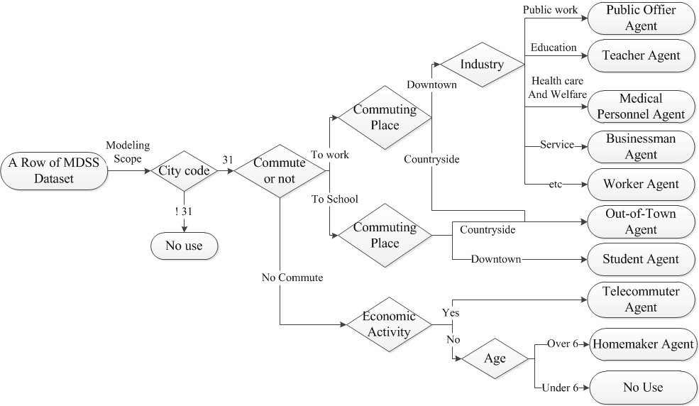

Figure 1. Flowchart of agent-type categorization with MDSS dataset

Time-Use Data on City Population

3.5

Many countries perform the time-use survey to gauge productivity, daily life, and infrastructure efficiency. We used the time-use survey provided by the Korean National Statistical Office. This survey provides the timetable of an ordinary individual in daily life. Particularly, this survey fits well into the MDSS dataset because the individuals are categorized by their occupations. Figure 2 is a facet of the time-use data, which specifies how much time an individual with a certain occupation spends performing a certain activity. The sleeping time is almost uniform for students, employees, and homemakers, whereas the commuting time and the leisure time are significantly different by occupations. This information provides two types of modeling information. First, from the time-use data, we enumerate activity states of agent types and their transitions. Second, the transition time for each state is also specified by the dataset.

3.6

Besides the activity-state duration by occupations, the time-use data provides individual-level data of a certain activity. Commuting behavior is important in analyzing and simulating traffic patterns, shopping-in behavior, and regional characteristics. Therefore, the time-use dataset provides a sampled set of individual commuting-time data: when they leave their workplace or home to commute. Figure 3 illustrates commute patterns of student agents and other agents. There are two peaks because the agents have to go back and forth between the home and workplace. Compared to the other agents, student agents have a more-concentrated commute period in the morning because every student's class starts at 9:00 a.m. in Korea. This individual record of commuting time suggests the distribution parameters, i.e., mean and variance, on what time the agent commutes in a virtual city.

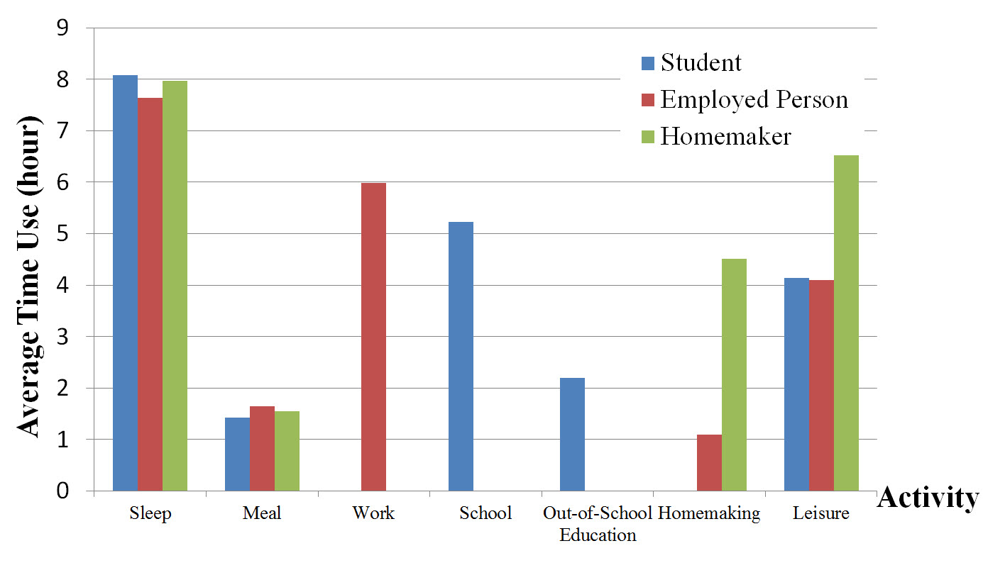
Figure 2. Time-use statistics of daily activity by student, employed person and homemaker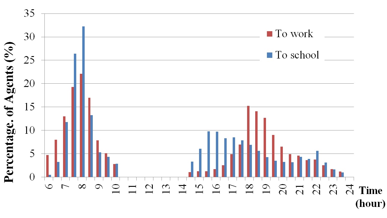

Figure 3. Time-use statistics of commute behavior by student agents and the other agent types

Geographic Information Data on City Environment

3.7

In addition to the agent models, we have environment data that captures the geospatial characteristics of Gwacheon. The data were downloaded from OpenStreetMap, see Figure 4, and a data-cleaning process followed because the data of Korean regions was significantly incomplete. We recovered 56 buildings of five different types and their geospatial locations. Further, we identified a road network that has 37 road segments and 31 junctions. The road network data were structured and stored as a graph data to be used by agents. The building data were not directly converted into the network data, yet the in-and-out of the buildings was connected to the closest road segment of the network. Three types out of the five building types are closely related to the simulations. First, the governmental buildings are specified as workplaces, so the worker agents commute to the locations. Second, the commercial buildings are located at the sides of road segments, so the passing-by agents can drop-in and shop. Third, the residential buildings are distributed across the city, and the agents start their daily activities from the residential buildings. These three types of buildings become the basic spots to create an origin-destination matrix for an individual agents, and the origin-destination matrix of a population may reveal which commercial areas may have more or less passing-by agents after the policy implementation.

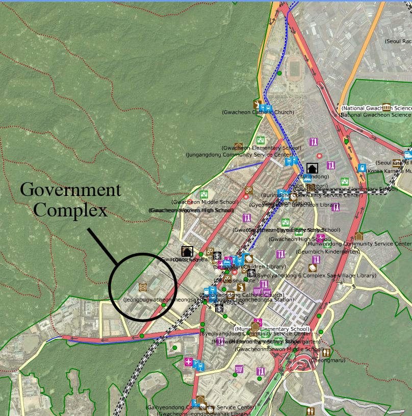
Figure 4. OpenStreetMap screenshot of city of interest, Gwacheon

Agent-Based Model Description

3.8

Since the scenario requires complex interactions between the city environment and individuals, we chose ABM as our modeling approach. Figure 5 shows the structure of our ABM. The model is mainly composed of largely two parts: the heterogeneous-agent models and the environment data. We formally modeled the agents and treated the environment as data objects that are used by agents. This limited the event generation and process of environment, but those were outside our modeling scope. We implemented our model with Repast Symphony 2.0^[1].

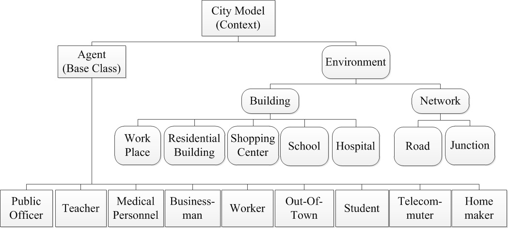
Figure 5. Agent-based model structure hierarchy; rectangles are models, and rounded rectangles are data objects

3.9

The agent models are built upon a base class that has basic functionalities of agents, such as shortest-path finding, agent generation, and agent removal. Our model depends heavily on the traffic behavior of agents, so we made a number of assumptions on modeling the shortest-path finding.

• Agents know the neighborhood, and they are able to find the shortest route with global map information.
• The global map information is just the information of the geospatial layout and road network; it does not include traffic flow speed at a certain time.

3.10

To implement the above shortest-path-finding behavior, we applied a simple Dijkstra algorithm to the implemented model. After implementing the base class, diverse agent types were implemented through the inheritance, and we continued the model description of our diverse agents, discussed in Section 3.3.

Formal Specification of Agent Behavior

3.11

Though the base function of agents is intuitive without a detailed explanation, the schedule of agent behaviors is a crucial part of the models that requires further explanation. One way of specifying agent behavior is through the utilization of flowcharts. However, the flowchart is an inadequate expression in the concrete formalism of models because there is only a weak consensus on symbols and arrows. Furthermore, the flowchart is useful in a brief description, but it is less useful in specifying the detailed timings of behaviors because it is impossible to specify the time advance in the flowchart. Similarly, the diagram of finite state machines suffers from a number of weaknesses. Though the finite state-machine diagrams are better than flowcharts in showing the state transition—which is a primary design of agent modeling—the diagrams still lack the timing of behavior, the perception-event handling, the action-event handling, and so on. We suspect that these shortcomings of agent-behavior representation are commonly derived from a lack of formalism in the agent-model description. Thus, we utilize one of the most well-known formalisms in the discrete event model, DEVS Formalism, to formally specify the agent behaviors in our model. Our ABM has no part of continuous time models, so it is a discrete-event model in the big picture. Therefore, our ABM can be specified by the DEVS formalism, which is known as a full, complete expression of a discrete-event model. Moreover, a DEVS diagram that is complete as well as intuitive would be a useful representation in the agent-behavior transitions.

3.12

In our model, agents make a decision on daily activities based on their agent type and current state. Figure 6–10 describes 1) the states, 2) their transitions guided by the external events, and 3) the outputs to the outside of the agent model. There are five types of agent behaviors varied by the agent types that come from the occupation date in the MDSS. Each of the first four diagrams describes the behaviors of student agent, out-of-town agent, homemaker agent, and telecommuter agent. The last diagram describes the behavior of commuting agents, which are the public officer agent, businessman agent, teacher agent, medical personnel agent, and worker agent. States in the diagram represents their current behaviors, and time advances that corresponds to their state indicates time duration for the associated behavior.

3.13

Agent types and the number of agents with an agent type were set by MDSS data, and by the defined agent types, agents' daily behaviors, such as where to visit and when to go, would be determined. Using MDSS data and Time-use data, we developed must-go buildings according to heterogeneous agent types, which indicates the buildings that an agent with a certain type should visit in a day (see Table 2). More specifically, each agent type should go to several types of buildings in its daily schedule. For example, in Figure 6, a student agent prefer to school, and academy, while a homemaker agent, in Figure 8, has no buildings that the agent must go. Also, for the variation in simulation, the alternatives of the mandatory schedules (i.e., going to must-go buildings) are designed. In Figure 6, a student agent can go to school with a higher probability (P_SC) or stay at home with a lower probability (P_H1) (i.e., P_SC >> P_H1). Such probabilities in the above figures are arbitrarily defined. When an agent decides to go to a building, the agent moves to the building through the road network model and stays there for a certain time duration, or time advance. Such duration time for the behaviors is fundamentally drawn from the time-use statistics described in Section 3.1.2.

3.14

When an agent goes over all must-go buildings, its mandatory schedules in a day is over so that the agent could have leisure time. The leisure time was categorized into two-folds: going to another places or taking a rest at home. For example, when a student agent moves around its school and academy, it could go to another places for its leisure time or go back home for taking a rest. In Figure 6, when the state of a student agent is Academy and its duration is over, the agent makes a decision to go to another place (with P_Sh1) or home (with P_H2). If an agent decides to go to another place, the agent can go around buildings except its must-go buildings and should go back home until its sleeping time that can be also derived from time-use data.. Such a design method is adopted to develop other agent types considering their must-go buildings and time-use data (see Figure 6–10) so that we could generate calibrated behaviors of the various agent types from the real data.

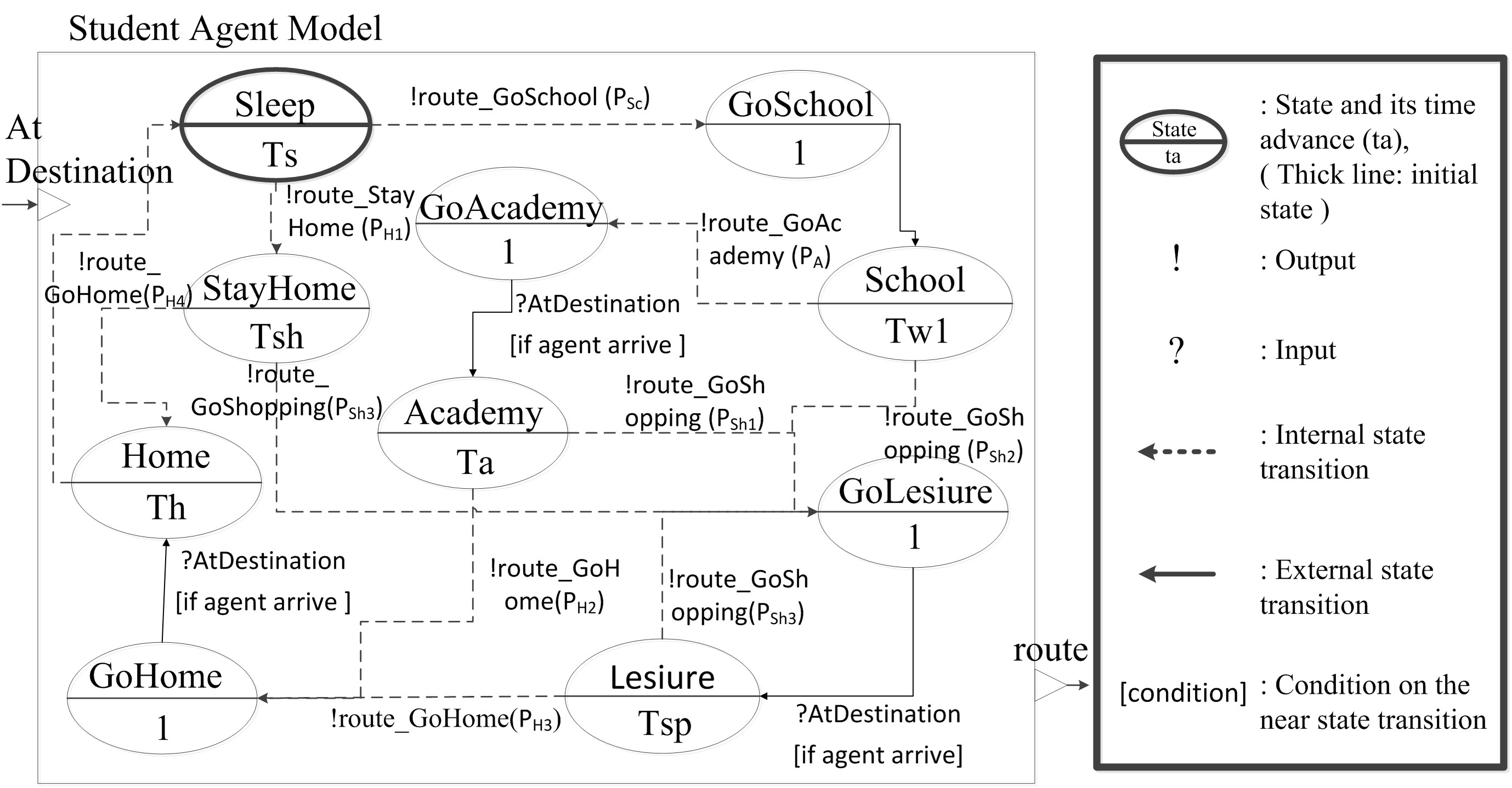
Figure 6. (Left) DEVS diagram for student agent's behaviors (states) and their time schedules (time advances) and (Right) notations on a DEVS diagram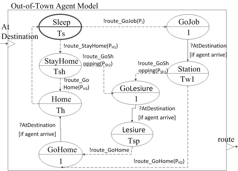

Figure 7. DEVS diagram for out-of-town agent's behaviors (states) and their time schedules (time advances)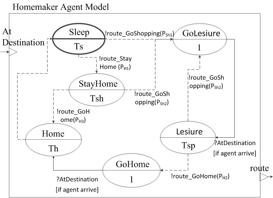

Figure 8. DEVS diagram for Homemaker agent's behaviors (states) and their time schedules (time advances)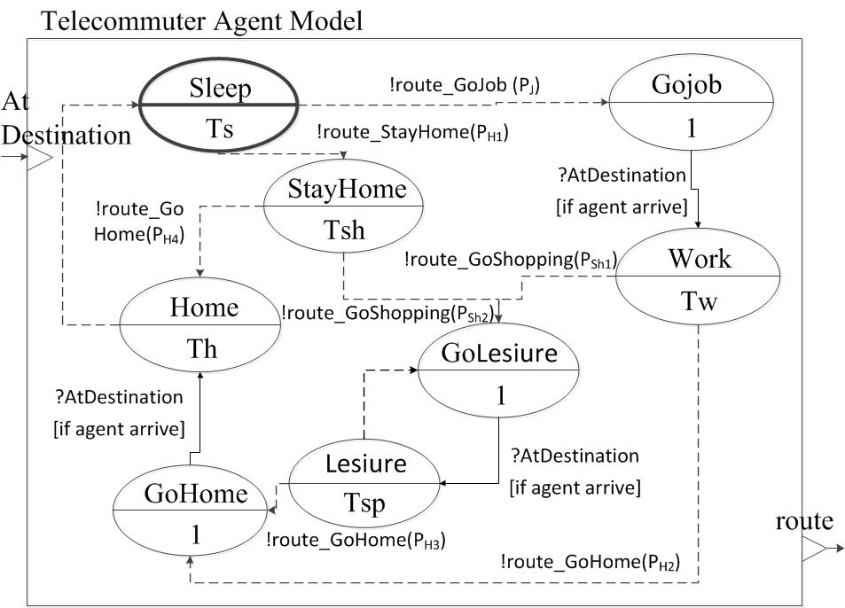

Figure 9. DEVS diagram for telecommuter agent's behaviors (states) and their time schedules (time advances)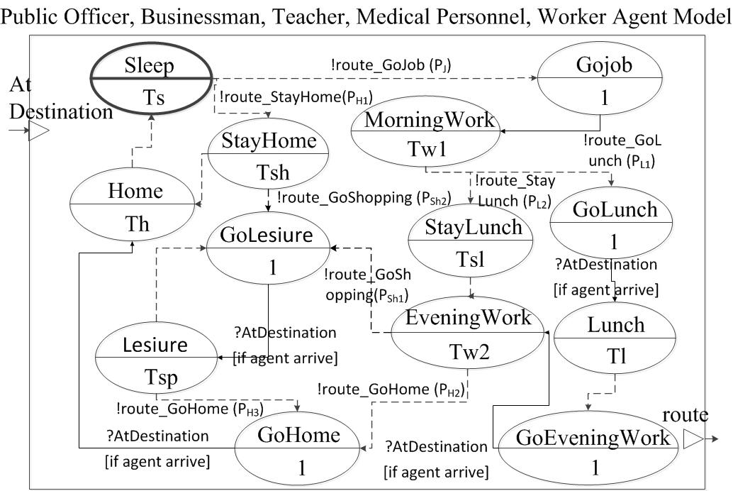

Figure 10. DEVS diagram for public officer, businessman, teacher, medical personnel, and worker agent's behaviors (states) and their time schedules (time advances)

Table 2: Must-go building lists according to heterogeneous agent types
Building Info.	Agent Type
Building Type	Number	Student	Out-of-town	Home maker	Tele commuter	Public officer	Business man	Teacher	Medical personnel	Worker
Public	1					O
Office	8				O		O			O
Shopping	8
Traffic	4		O
Apartment	10	O	O	O	O	O	O	O	O	O
Hospital	2								O
Restaurant	9					O	O	O	O
Academy	4	O						O
School	10	O						O
Total	56

Model Summary and Virtual Experiment Design

3.15

We built our ABM of daily activities with a focus on weekday working and shopping behavior to assess the impact of the population relocation on the city commerce. While the previous sections described the model architecture and the inside of the agents, Table 3 enumerates the utilized datasets and generated output for the analysis. We calibrated our agent activities by the MDSS dataset and the time-use dataset. We obtained the 5% sample data of overall population in Gwacheon city from MDSS, which contains only 1,189 members of the population. As the 1,189 population is too small to evaluate the impact on the commerce, we generated 2,154 agents in our model, which is twice the size of the population data. The desired output is the potential shop-in behavior counts of each commercial building in Gwacheon.

Table 3: List of input variables, output variables, and parameters of our agent-based model
Type	Name	Implication
Input	MDSS Dataset	Given attributes of each agent, agent type is determined, and the daily schedule is generated by the type of agent.
	Time-Use Dataset	The daily time consumption on a certain activity state for a certain type of individual
	GIS Dataset	Information of roads and buildings about coordinates, type, and identification
Output	Number of Passing-by Agents	The count of passing-by agents for each building to gauge the commerce activities
	Number of Agents on Road Segment	The count of agents on a certain road segment to gauge the traffic status
Parameter	Reduction Ratio	Portion of relocating public officers over all of the public officers in Gwacheon city
	Commute Ratio	Portion of public officers who commute between Gwacheon and new city without moving out over all of the relocating public officers
	Family Move	Boolean value indicating whether a public officer would move out with his family or not
	Transportation Speed	The speed of walking is 1, and others are x times faster than walking (walk = 1, bike = 3, bus = 8, car = 10)
	Simulation time	Total simulation time (default = 24 hours)
	Initial Position of Agent	Determine the house of agent randomly before the simulation (default = random assignment with the MDSS dataset, see Section 3.3.)
	Required Place of Agent	Determine the mandatory place for agent depending on its type (default = random assignment with the MDSS dataset, see Section 3.3.)
	Activity Duration	Activity duration of agent depends on its statistics (default = time-use statistics in Section 3.1.2.)

3.16

In the simulation, the model counts the passing-by agents to gauge the size of local populations at a certain location, and we assume that the counts on passing-by agents would negatively affect to the city commerce. This assumption is not an originative one because the relationship between population in a local area and the local economy was researched in numerous works (Kuznets 1967; Simon 1986; Becker, Glaeser & Murphy 1999; Tsen & Furuoka 2005). For example, Tsen and Furuoka (2005) investigated the relationship between population and economic growth in Asian economies. Also, Fesser and Sweeney (1999) examined significant forms of economic distress that accompanied out-migration and population loss in U.S. communities from the same viewpoint of ours. The counts on passing-by agents depend on the traffic status of the road network, so the number of agents on a certain road segment is also counted.

3.17

Table 4 is the virtual experiment design to establish scenarios of interest and estimate the impact of the relocation policy. The policy to be implemented will relocate the workplace for public officers in Gwacheon to the other city, so the public officers and their family in Gwacheon city are subject to considering the movement by the relocation policy. Once the policy is executed, we could estimate three possible cases of the public officers dependent on several conditions:

• When the relocation policy is executed, some of the public officers should relocate to new administrative city
• Among the relocating public officers, some would move out from Gawcheon city, but others would commute between Gwacheon and the new city
• Among the moving out public officers, some would move out with their family, but others would move alone

3.18

Based on the three possible cases, we setup three experimental variables: reduction ratio, commute ratio, and family move. Reduction ratio indicates a portion of the relocating public officers. If the reduction ratio is 0.1, 10% of public officers in the city should relocate to the new administrative city. Commute ratio describes a portion of the relocating public officers who commute between Gwacheon city and the new city without moving out. If the commute ratio is 0.0, all of the relocating public officers would move out from Gwacheon city. Family move represents whether a public officer's family would go with him or not when he decides to move out. In our virtual experiments, we developed seven cases of reduction ratio, five cases of commute ratio and two cases of family move (see Table 4). Thus, we came up with 70 simulation cases by the full-factorial experimental design and added one more simulation case (i.e., baseline) with no relocations. All of the experiments were repeated 20 times to prevent the effects of randomness in our model.

Table 4: Virtual experiment design of scenario of interests
Experiment Variable Name	Experiment Design	Implication
Reduction Ratio	0.1, 0.2, 0.3, 0.4, 0.5 0.6, or 0.7 (7 cases)	Portion of relocating public officers over all of the public officers in Gwacheon city
Commute Ratio	0.0, 0.25, 0.50, 0.75, or 1.00 (5 cases)	Portion of public officers who commute between Gwacheon and new city without moving out over all of the relocating public officers
Family Move	True or False (2 cases)	Boolean value indicating whether a public officer would move out with his family or not
Total Number of Experiment Cells	70 experiment cells + 1 baseline cell (= 7 * 5 * 2 + 1 cases)	Each cell is replicated 20 times

Results

4.1

We analyzed the policy impact with the described ABM and the experiment design. First, this section presents the results of the policy analysis which is the major objective of this paper. The results of the policy analysis are provided visually as well as with a statistical significance test. Second, this section illustrates the statistical validation results on the model. We present how we gathered the validation dataset and how we statistically computed the correlation between the simulated world and the real world.

Result on Relocation Policy Analysis

4.2

We performed a virtual experiment with our model and experiment design. To assist the intuitive understanding of the result, we provided a visualization of simulation runs. After the visualization, we investigated the significance of changes on the passing-by agents at the building level. One merit of utilizing the ABM is the micro-level analysis of simulation outputs, so we observed which areas would be affected more than the other areas.

Illustration on Model Execution

4.3

Our ABM simulates the local population's daily activities with a focus on traffic and shopping-in behavior. Figure 11 shows a list of screenshots at 6am, 8am, 2pm, and 6pm in the simulation world. The agent types are color-coded in the screenshots, and the buildings are geospatially distributed in the region. Figure 3 from the time-use dataset specifies that there is a smaller range of time for going to the workplace compared to going home in the commuting activities. Therefore, our model shows the heavier traffic at 8am compared to the traffic at 6pm. At 6am, there is little traffic because of random time-advance adjustment for some agents. At noon, agents who do not commute come out for shopping and other activities.

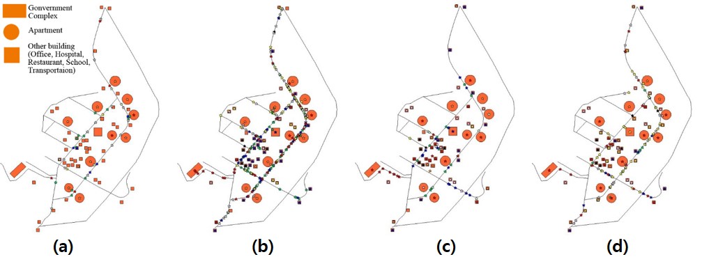
Figure 11. Simulated daily activities of local population at 6am (a), 8am (b), 2pm (c), and 6pm (d) in the simulated city

4.4

Figure 12 shows the impact of reducing passing-by agents at commercial buildings of interest. The 17 buildings were selected by if they were related to shopping, dining, or leisure activities, which would be the commercial buildings in the city. Figure 12 shows the nine cases out of 70 experimental cells in Table 4. When the family does not relocate, the impact to the counts of passing-by agents was minimal. Therefore, we selected nine representative cells when the family does not relocate. We observed that the buildings were affected differently by the commute ratio and the reduction ratio. Furthermore, the geographic locations of buildings influenced the impact as well. For instance, the cell with a high reduction ratio and low commute ratio showed a greater reduction than the cell with a high reduction ratio and high commute ratio because the local population diminishes less with a higher commute ratio. The commuting behavior will lead the agents to the highway interchange at the north of the city, so some buildings in the way are almost the same before the policy is implemented.

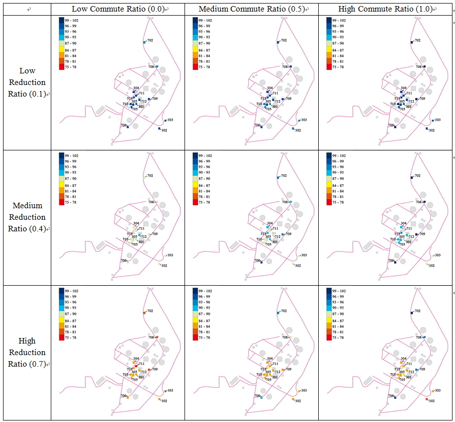
Figure 12. Reduction rate of the number of passing-by agents with various experimental variable settings; north is up, and the percentage indicates the reduction of passing-by agents compared to the baseline

4.5

Figure 13 illustrates the aggregated impacts of the city commerce through diverse factors. Figure 13 implies that the relocation will not affect much unless it is accompanied by the family relocation. This relocation of the family is much more significant than varying the relocation ratio of the public officers. Actually, this estimation is already being observed in Gwacheon because there are reports questioning the impact of the relocation policy without whole family movements.

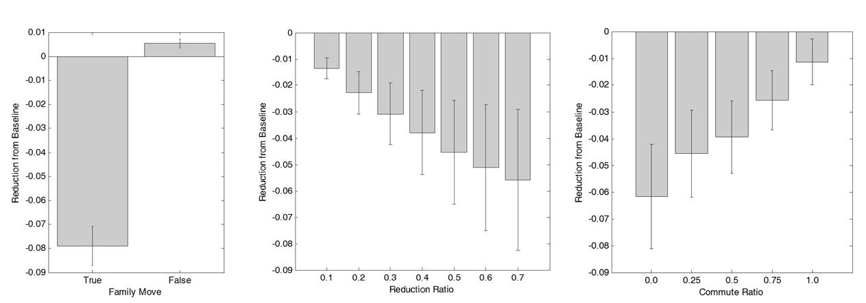
Figure 13. Percentages of reduced passing-by agents compared to the baseline (Left) marginalized by family move parameter, (Center) marginalized by reduction ratio, and (Right) marginalized by commute ratio (marginalization: integrating or summing out results from three parameters to the result of one parameter for concentrating on the effect by each parameter independently)

Statistical Analyses on City Commerce

4.6

In our simulations, the counts of passing-by agents of commercial buildings vary by four factors: building locations, family move, reduction ratio, and commute ratio. To statistically evaluate the significance of these factors, we developed a meta-model that explains the significance of the factors in determining the counts. The meta-model is a multivariate linear regression between the four factors and the counts of passing-by agents. Two factors, the building and the family move, are categorical variables, so we created two corresponding sets of variables by omitting one case for each of the sets. Table 5 describes the details of the meta-modeling result. Because we standardized the coefficients, we can compare the sensitivity of changing variables to increase the counts. As illustrated in Figure 9, the counts decrease when the families move, the reduction ratio increases, and the commute ratio decreases. Table 5 indicates that the strengths of the three factors are in the order of family move, commute ratio and reduction ratio by observing the standardized coefficients and the P-value indicates the robustness of the interpretations. When we compare the three factors to the commercial building locations, most of the locations have a stronger influence to the counts than the family move, the reduction ratio, and the commute ratio. This means that the building locations will be the strongest factor in determining the rise and fall of the commercial merits, and this is illustrated in Figure 12.

4.7

Besides the meta-modeling, we performed an analysis of variance (ANOVA) test on the factors and the counts of passing-by agents. Table 6 shows the influence from the treatments, which are experimental variables, to the counts. The analysis result is consistent with the meta-model. The building location is the major treatment to change the counts. Then, the family move, the commute ratio, and the reduction ratio have the influence to the counts in the order of the strengths.

Table 5: Meta-model of passing-by counts with linear regression of passerby counts by buildings of interest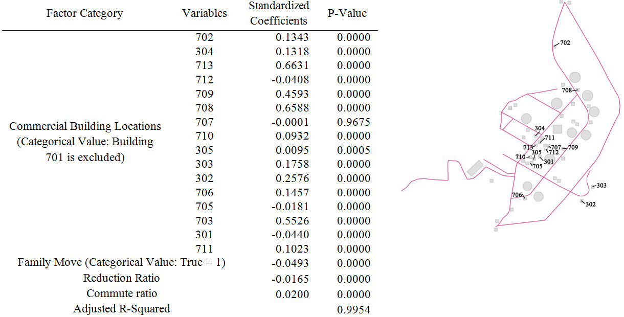

Table 6: ANOVA to show factor significance between the experimental variables and the counts of the passing-by agent
Variables	'Sum Sq.'	'd.f.'	'F'	'Prob>F'
Commercial Building Locations	4.30E+09	1.60E+01	15820.3738	0.0000
Family Move	1.05E+07	1.00E+00	620.6110	0.0000
Reduction Ratio	1.19E+06	6.00E+00	11.7019	0.0000
Commute Ratio	1.75E+06	4.00E+00	25.8057	0.0000
'Error'	1.97E+07	1.16E+03
'Total'	4.34E+09	1.19E+03

Result of Model Validation Analysis

4.8

This simulation study was designed in the middle of 2012 when the policy was about to be executed. In Aug, 2013, we surveyed the actual changes in Gwacheon. This study focuses on the impact of the relocation on the commercial aspect, so we investigated the rent rate changes of the simulated buildings in the real world. The direct measure of commercial status would be a sales amount of shops and malls in the region, but such information is difficult to collect in the city-wide area. Therefore, we collected the indirect measure, i.e., the rent rate of the buildings, showing the changes in the commercial aspect, and this measure is easier to survey. However, objectively recording the rent rate of commercial buildings was not an easy task because the contracts were not made often and because the exact rate was not publicly available, which was very different from finding the rent rate for residences. Therefore, we contacted 11 major real-estate agencies and performed the surveys on the rents of the buildings. Because there were no responses from some of the interviewees, we recovered only five survey returns. Furthermore, out of 17 buildings of interest in the simulation, three buildings were not available for renting spaces for commercial purposes, so 14 buildings became the targets of validation.

4.9

Figure 14 and Figure 15 shows the visual comparison between the measures from the real world and the simulations. We contrasted the surveyed rent rate and the average counts of passing-by agents by commercial buildings of interest. It is difficult to see a strong correlation between the two, yet the scatter plots show a slight positive correlation between the two sets of metrics. Whereas there seems to be a positive correlation, some buildings, Building 711, 706, and 302, are deviated from the fitted line.

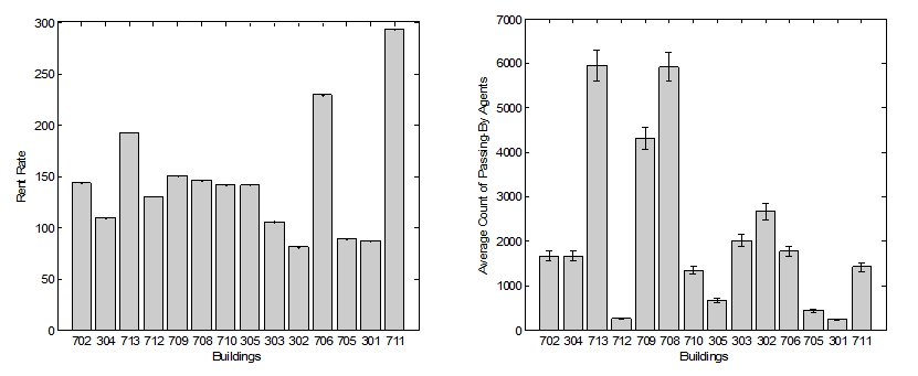
Figure 14. (Left) Surveyed rent rates by buildings in the real world and (Right) average count of passing-by agents in the simulations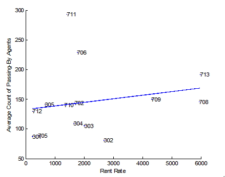

Figure 15. Scatter plot and a linear fitted line between the simulation result and the real world survey

4.10

Since we cannot confirm the correlation with only the visualization of the two distributions, we calculated the correlations between the two distributions. Specifically, we calculated the correlations between the surveyed distribution and each virtual experiment cell, which resulted in 70 sets of correlation results. Also, we calculated three different correlations: Pearson correlation, Spearman's rank correlation, and Kendall's tau rank correlation. We included the rank correlations because simulation results with correct prediction in ranks, not the continuous value distribution, can be useful in the real world policy analyses. Table 7 shows the summary of this correlation analysis. When we include every building of interests, the value correlation is 20.68%, and the rank correlation is 45.49%. Considering that this is a social simulation that is very difficult to achieve high validation, we think that this is an average quality for the validation. When we exclude the buildings that are deviating from the fitted line in Figure 15, the value correlation becomes 48.3%, and the rank correlation becomes 85.45%. This would be a good quality of validation considering the difficulty of the validation of social simulations. Besides the statistical validation result, we traced which virtual experimental cells resulted in the maximum correlation. This parameter trace result might tell us the actual settings of the real world. For example, when the experimental cells generating the maximum Spearman's rank correlation simulates when the families do not relocate, the reduction rate is 0.7, and the commute ratio is 0.5.

Table 7: Correlation analysis between the surveyed rent rate and the simulated passing-by agent counts
	14 Buildings	11 Buildings (Excluding outliers: Building 711, 706, and 302)
	Max. Correlation Value	Simulation Setting of Max. Correlation	Max. Correlation Value	Simulation Setting of Max. Correlation
		Family Move	Reduction Ratio	Commute Ratio		Family Move	Reduction Ratio	Commute Ratio
Pearson Correlation	0.2068	True	0.6	1.0	0.4830	True	0.3	0.75
Spearman's Rank Correlation	0.4549	True	0.6	1.0	0.8545	False	0.7	0.5
Kendall's Tau Rank Correlation	0.3187	True	0.6	1.0	0.6727	False	0.7	0.5

Conclusions

5.1

We studied the impact of the public officer's relocation policy to the commerce of Gwacheon city. Our agent-based model is calibrated with the micro-population dataset, the time-use dataset, and the geospatial environment of the city. The analysis results estimate that the relocation will reduce the city commerce significantly in three cases: when the families of the public officers relocate, when the reduction ratio gets higher, and when the commute ratio becomes lower. While the city-wide commerce would be damaged in general, the magnitude of the impacts will differ by the buildings, particularly by the geospatial locations of commercial buildings. When we gauge the strengths of the factor influence to the damage, the building location would be the most significant factor in determining the impact magnitude. To validate this result, we surveyed the rent rate of the commercial buildings as a proxy measure to observe the damage to the city commerce. While there are outlier buildings in the validation, the value correlation is 48.3%, and the rank correlation is 85.45%.

5.2

Many policies are designed and implemented for a greater good and a strategic purpose. This relocation policy of the government complex is intended to divert a small function of Seoul to a distant city, so the over-population and its accompanying problems could be resolved in the process. However, this policy makes a profound impact on the affected population: the families that needs to relocate, the public officers who might commute for two hours a day, and the local shops and malls with reducing sales. Policy makers might need a tool that enables them to foresee the outside effects of their policies, and this simulation would be such a tool.

Acknowledgements

Supports from the Public welfare & safety research program through the National Research Foundation of Korea (NRF) (2012-0029881)

Notes

¹This model can be found at https://www.openabm.org/model/4345/version/1/view

References

ARENTZE, T. A., Pelizaro, C. & Timmermans, H. J. P. (2005). Implementation of a model of dynamic activity-travel rescheduling decisions: an agent-based micro-simulation framework. Proceedings of the Computers in Urban Planning and Urban Management Conference, 48.

ARENTZE, T. A. & Timmermans, H. J. P. (2004). Albatross – a learning based transportation oriented simulation system. Transportation Research Part B: Methodological, 38(7), 613–633. [doi:10.1016/j.trb.2002.10.001]

BAE, J. W., Lee, G. & Moon, I.-C. (2012). Formal specification supporting incremental and flexible agent-based modeling. Proceedings of the 2012 Winter Simulation Conference (pp. 1–12). [doi:10.1109/WSC.2012.6465163]

BATTY, M. (2004). Cities and Complexity: Understanding Cities with Cellular Automata, Agent-based Models, and Fractals. MA: MIT press.

BECKER, G. S., Glaeser, E. L. & Murphy, K. M. (1999). Population and economic growth. American Economic Review, 145–149. [doi:10.1257/aer.89.2.145]

BECKX, C., Int Panis, L., Arentze, T., Janssens, D., Torfs, R., Broekx, S. & Wets, G. (2009). A dynamic activity-based population modelling approach to evaluate exposure to air pollution: methods and application to a Dutch urban area. Environmental Impact Assessment Review, 29(3), 179–185. [doi:10.1016/j.eiar.2008.10.001]

BURGESS, E. W. (2008). The Growth of the City: An Introduction to a Research Project (pp. 71–78). Springer US. [doi:10.1007/978-0-387-73412-5_5]

CARLEY, K. M. (2002). Computational organization science: A new frontier. Proceedings of the National Academy of Sciences, 99(suppl 3), 7257–7262. [doi:10.1073/pnas.082080599]

CARLEY, K. M., Fridsma, D. B., Casman, E., Yahja, A., Altman, N., Kaminsky, B. & Nave, D. (2006). BioWar: scalable agent-based model of bioattacks. IEEE Transactions on Systems, Man, and Cybernetics - Part A: Systems and Humans, 36(2), 252–265. [doi:10.1109/TSMCA.2005.851291]

EPSTEIN, J. M. (1996). Growing Artificial Societies: Social Science from the Bottom Up, (pp. 1–20). Brookings Institution Press.

FESSER, E. J. & Sweeney, S. H. (1999). Out-migration, Population Decline, and Regional Economic Distress (p. 80). Washigton, DC.

FILATOVA, T., Parker, D. & Van der Veen, A. (2009). Agent-based urban land markets: agent's pricing behavior, land prices and urban land use change. Journal of Artificial Societies and Social Simulation, 12 (1) 3: https://www.jasss.org/12/1/3.html.

FONOBEROVA, M., Fonoberov, V. A., Mezic, I., Mezic, J. & Brantingham, P. J. (2012). Nonlinear dynamics of crime and violence in urban settings. Journal of Artificial Societies and Social Simulation, 15(1), 2.

FORRESTER, J. W. (1971). Counterintuitive behavior of social systems. Theory and Decision, 2(2), 109–140. [doi:10.1007/BF00148991]

GUO, H. C., Liu, L., Huang, G. H., Fuller, G. A., Zou, R. & Yin, Y. Y. (2001). A system dynamics approach for regional environmental planning and management: a study for the Lake Erhai Basin. Journal of Environmental Management, 61(1), 93–111. [doi:10.1006/jema.2000.0400]

HARRIS, C. D. & Ullman, E. L. (1945). The nature of cities. The Annals of the American Academy of Political and Social Science, 242(1), 7–17. [doi:10.1177/000271624524200103]

HOLZER, R. & de Meer, H. (2008). On modeling of self-organizing systems. Proceedings of the 2nd International ICST Conference on Autonomic Computing and Communication Systems (pp. 1–6). Turin, Italy. [doi:10.4108/ICST.AUTONOMICS2008.4671]

HOYT, H. (1939). The structure and growth of residential neighborhoods in American cities (p. 178). Washington, D.C: U.S. Govt.

JUN, M. J. (2007). Korea's public sector relocation: Is it a viable option for balanced national development? Regional Studies, 41(1), 65–74.

KANEDA, T. & Yoshida, T. (2012). Simulating shop-around behavior. Proceedings of the 2012 Symposium on Agent Directed Simulation (p. 8). Orlando, Florida: Society for Computer Simulation International.

KUZNETS, S. (1967). Population and economic growth. Proceedings of the American Philosophical Society (pp. 170–193).

MARSHALL, J. N., Bradley, D., Hodgson, C., Alderman, N. & Richardson, R. (2005). Relocation, relocation, relocation: assessing the case for public sector dispersal. Regional Studies, 39(6), 767–787. [doi:10.1080/00343400500213663]

MATTHEWS, R. B., Gilbert, N. G., Roach, A., Polhill, J. G. & Gotts, N. M. (2007). Agent-based land-use models: a review of applications. Landscape Ecology, 22(10), 1447–1459. [doi:10.1007/s10980-007-9135-1]

MOON, I. C. & Carley, K. M. (2007). Modeling and simulating terrorist networks in social and geospatial dimensions. IEEE Intelligent Systems, 22(5), 40–49. [doi:10.1109/MIS.2007.4338493]

OTTER, H. S., van der Veen, A. & de Vriend, H. J. (2001). ABLOoM: Location behaviour, spatial patterns, and agent-based modelling. Journal of Artificial Societies and Social Simulation, 4 (4) 2: https://www.jasss.org/4/4/2.html.

RATHI, A. K. & Solanki, R. S. (1993). Simulation of traffic flow during emergency evacuations. Proceedings of the 1993 Winter Simulation Conference (pp. 1250–1258). New York, New York, USA: ACM Press.

RODRIGUE, J.-P., Comtois, C. & Slack, B. (2011). The geography of transport system. Journal of Urban Technology, 18(2), 99–101. [doi:10.1080/10630732.2011.603579]

SCHWARZ, N., Kahlenberg, D., Haase, D. & Seppelt, R. (2012). ABMland - a tool for agent-based model development on urban land use change. Journal of Artificial Societies and Social Simulation, 15 (2) 8: https://www.jasss.org/15/2/8.html.

SIMON, J. L. (1986). Theory of Population and Economic Growth. Oxford United Kingdom Basil Blackwell.

SMITH, L., Beckman, R. & Baggerly, K. (1995). TRANSIMS: Transportation analysis and simulation (No. LA-UR-95-1641).

TESFATSION, L. (2002). Agent-based computational economics: growing economies from the bottom up. Artificial Life, 8(1), 55–82. [doi:10.1162/106454602753694765]

THÜNEN, J., Wartenberg, C. M. & Hall, P. (1966). Von Thünen's Isolated State. London: Oxford: Pergamon press.

TSEN, W. H. & Furuoka, F. (2005). The relationship between population and economic growth in Asian economies. ASEAN Economic Bulletin, 314–330. [doi:10.1355/AE22-3E]

WADDELL, P. (2002). UrbanSim: modeling urban development for land use, transportation, and environmental planning. Journal of the American Planning Association, 68(3), 297–314. [doi:10.1080/01944360208976274]

ZHANG, X. H., Zhang, H. W., Chen, B., Chen, G. Q. & Zhao, X. H. (2008). Water resources planning based on complex system dynamics: a case study of Tianjin city. Communications in Nonlinear Science and Numerical Simulation, 13(10), 2328–2336. [doi:10.1016/j.cnsns.2007.05.031]