Abstract

The VirtualBelgium project aims at developing an understanding of the evolution of the Belgian population using agent-based simulations and considering various aspects of this evolution such as demographics, residential choices, activity patterns, mobility, etc. This simulation is based on a validated synthetic population consisting of approximately 10,000,000 individuals and 4,350,000 households located in the 589 municipalities of Belgium. The work presented in this paper focuses only on the mobility behaviour of such large populations and this is simulated using an activity-based approach in which the travel demand is derived from the activities performed by the individuals. The proposed model is distribution-based and requires only minimal information, but is designed to easily take advantage of any additional network-related data available. The proposed activity-based approach has been applied to the Belgian synthetic population. The quality of the agent behaviour is discussed using statistical criteria extracted from the literature and results show that VirtualBelgium produces satisfactory results.

Keywords:

Micro-Simulation, Activity Chains, Transport Demand Forecasting, Nationwide Model, Large Population Simulation, Non Geo-Localized Data

Introduction and motivation

1.1

Activity-based models form a class of travel demand forecasting models originally based on the ideas of Hägerstrand (1970) and Chapin (1974). These were proposed as an alternative to the classical four-stage trip-based models for travel demand forecasting, the drawbacks of which were by then well identified (Dickey 1983; Domencich & McFadden 1975; Spear 1977; Oppenheim 1995). Activity-based approaches rely on the paradigm that people travel to carry out activities they need or wish to perform. Such models reflect the scheduling of activities performed by individuals in time and space. The sequence of activities, also named activity chains or patterns, becomes then the relevant unit of analysis. This approach is now widely accepted and continues to attract a lot of attention.

1.2

Activity-based models can be classified into at least four families. The first two are discrete choice models (Adler & Ben-Akiva 1979; Bhat & Koppelman 1999; Bradley et al. 2010; Bhat et al. 2004) and mathematical programming techniques (Gan & Recker 2008). They have the drawbacks that the former approach may requires an extremely large choice set in order to capture a sufficient fraction of feasible mobility patterns, while the latter may not be tractable as the decision processes formulation may be extremely complex. This last issue also appears in structural equation modelling techniques, another family of activity-based models, which is rather confirmatory than explanatory. We refer the reader to Golob (2003) for a review of contributions using this approach and to Hoe (2008) for an insight on its limitations. Finally, the fourth model family exploits the advent of high performance computing by using massive multi-agent micro-simulations in order to reproduce behaviours within a complex system, such as the mobility behaviours of a large population (Kitamura et al. 1997).

1.3

It has been noted that "micro-simulation ... is drawing attention as a new approach to travel demand forecasting" (Miller 1997), and several operational micro-simulators for activity scheduling are currently in use. Examples include ALBATROSS (Arentze & Timmermans 2000) for the Netherlands, TASHA (a part of the ILUTE simulator, Salvini & Miller 2005) for the Greater Toronto Area, SAMS and AMOS (Kitamura et al. 1996). A review and comparison of various micro-simulators and discrete choice models for activity-based modelling can be found in Goran (2001). These approaches typically implement the first three steps (generation, distribution and modal choice) of the traditional four-stage model. The last step, namely traffic assignment, can be handled with dynamic traffic assignment procedures, the adoption of which has been made easier by the development of powerful open source agent-based simulation systems such as MATSim (see http://www.matsim.org, accessed on January 2015), used by Meister et al. (2010) in travel demand forecasting for Switzerland, Urbansim (Waddell 2002) and Transim (Nagel et al. 1999).

1.4

Even though all these approaches have demonstrated their usefulness, they typically require, in addition to a complete description of the road network, an a priori localisation of every housing unit, service, shop... This turns out to be a strong requirement: indeed, although this information can often be gathered for a particular city or even a district of a country, the geo-localisation process is far more complex and cumbersome for a whole country and may not be feasible. This issue motivates our interest in the design of an alternative methodology obviating this limitation by relying on statistical distributions, but flexible enough to use all information available and making it suitable for nationwide application. Hence the proposed methodology represents a major departure from previous activity-based models since no geolocation data is necessary. In addition, weaker data requirements imply that this proposal is easily transferable to any study area and this represents a major advantage over the existing approaches.

1.5

The approach taken here is the micro-simulation of Belgian population mobility behaviours as a part of the VirtualBelgium integrated simulator. The agents are derived from a synthetic population previously generated and validated (Barthélemy & Toint 2013). The proposed activity scheduling model is a three step procedure: first, a set of feasible activity chains is generated for every agent type; a chain is then assigned to every individual agent of the simulation using a randomized model; and all characteristics of all the activities of the chain are finally determined based on statistical distributions. The outputs of the model can then be processed using MATSim for dynamic traffic assignment, if required. VirtualBelgium's activity-based model relies mainly on data extracted from the Mobel national mobility survey conducted in Belgium (Hubert & Toint 2002) and the OpenStreetMap project (Haklay & Weber 2008).

1.6

The remainder of this paper is organized as follows. Section 2 introduces VirtualBelgium's framework, data sources, agents and the activity chains which they can perform. In Section 3, we detail the proposed method for assigning activity chains to individual agents using statistical distribution. We then present in Section 4 the results obtained with this methodology when applied to VirtualBelgium. Limitations of the model, concluding remarks and future perspectives are discussed in Sections 5 and 6.

VirtualBelgium: a multi-agent micro-simulation for Belgium

2.1

Describing our activity chain generator is difficult without introducing the basic elements of the framework in which these patterns are exploited. We therefore start with a brief outline of VirtualBelgium, a research project for simulating mobility behaviour and demographic evolution of the Belgian population using a multi- agent approach, based on the Repast HPC 2.0 (Collier & North 2012) and MATSim frameworks. The project, detailed in (Barthélemy 2014), is open-source and hosted on the SourceForge platform where it can be downloaded at the following address: http://virtualbelgium.sourceforge.net.

2.2

The agents of interest in VirtualBelgium consist of individuals in a population P = (I, H) of approximatively 10,000,000 people ∈ I gathered in 4,350,000 households ∈ H. Each of these household is located in one of the 589 Belgian municipalities. There is a number of spatial micro-simulation methods used to derive a synthetic population of agents for a particular study area when a fully disaggregate data set is not available due to stringent privacy laws or cost reasons (Hermes & Poulsen 2003; Tanton & Edwards 2012, and Tanton 2014 present a good review of the techniques available). In our context, a synthetic population for Belgium was created using a validated sample-free generator fully detailed in Barthélemy & Toint (2013). Since the resulting artificial population is reliable, we can make the assumption that the population does not restrict VirtualBelgium's accuracy.

2.3

As agent attributes we have chosen characteristics which are known to significantly influence travel behaviour (Avery 2011; Hubert & Toint 2002; Cornelis et al. 2012). Individual and household attributes are presented in Tables 1 and 2, respectively. Even though the number of attribute is limited (due to the input data available for generating the synthetic population), it has been previously shown that they significantly influence travel behaviour (Avery 2011; Hubert & Toint 2002; Cornelis et al. 2012). The education level and socio-professional status can approximate important missing attributes such as income level and type of employment. Nevertheless it is clear that the lack of household residential municipality type (urban/rural/suburb) represents a limitation on the VirtualBelgium input data as it affects travel behaviour.

Table 1: Individuals' characteristics.
Attribute	Values
Gender	male; female
Age class	0-5; 6-17; 18-39; 40-59; 60+
Age	an integer from 0 to 110
Socio-professional status	student; active; inactive
Education level	primary; high school; higher education; none
Driving license ownership	yes; no

Table 2: Households' characteristics.
Attribute	Values
Type	single man alone single woman alone single man with children (and other adults) single woman with children (and other adults) couple without children (and other adults) couple with children (and other adults)
Number of children	0 to 5
Number of other adults	0 to 2

2.4

The mobility patterns of a given individual evolve together with his/her socio-demographic characteristics. Therefore it is interesting to implement procedures representing an evolution process for the population of interest in order to forecast the travel demand in the future as well as the socio-demographic evolution of Belgium. For instance, an individual agent gets older, gives birth to new agents, dies, moves out, finds a mate, divorces, etc.

2.5

Consequently VirtualBelgium contains two complementary simulation module sets, namely, the traffic and the socio-demographic simulators as illustrated in Figure 1. First the initial agents are generated, and then the traffic simulator module is executed. The socio-demographic evolution module can afterwards be applied to the agents to forecast a future population for which the travel demand could be estimated by applying the traffic simulator. It should be noted that the temporal resolution depends on the module: one tick of the traffic simulation corresponds to one day in the agents' life while it corresponds to one year for the evolution module.

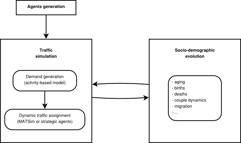
Figure 1. VirtualBelgium modules.

2.6

An overview of VirtualBelgium's structure, which follows the standard agent-based programming approach (van Dam et al. 2012), is illustrated on the class diagram of Figure 2. The agents (Individual and Household classes), their actions and interactions are ruled by a scheduler (belonging to the Model class). The agents' environment is the Belgian road network (Network class).

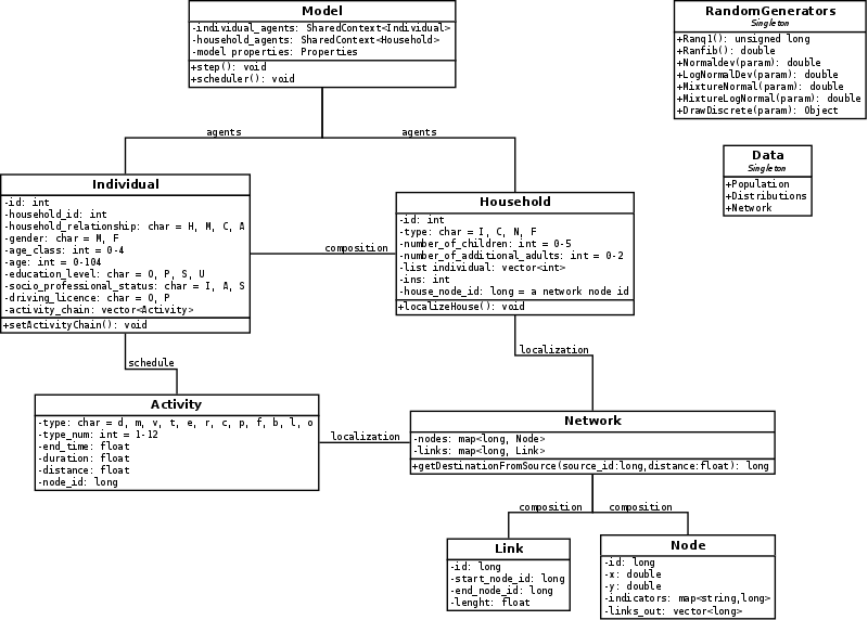
Figure 2. Class diagram.

2.7

It can be seen that VirtualBelgium is an evolutionary platform. Indeed its modular conception and agent-based structure facilitate the implementation of additional (interaction) models and the design of new in silico experiments.

2.8

Since the scope of this work is focused on mobility behaviour and more specifically on the modelling of the individuals' activities, the traffic assignment, agent generation and evolution processes will not be further discussed.

Activity chains, general assumptions and data source

2.9

The activity chain data used by VirtualBelgium is derived from the Mobel 2001 mobility survey conducted in Belgium. These surveys highlighted 12 base activities:

• pick up/drop (d);
• staying home(m);
• work related visit(v);
• work(t);
• school(e);
• eating outside(r);
• shopping(c);
• personal reason(p);
• visiting relatives(f);
• going for a walk (b);
• leisure activity (l);
• other(o).

2.10

Each activity is also characterized by a duration and a localization within the Belgian road network. Such a network is extracted from OpenStreetMap and is defined by the pair G = (N, L), where N and L correspond, respectively, to the sets of nodes and links which can be thought of as crossroads or junctions and sections of roads, respectively. An activity localization is then a node of the network.

2.11

It should be noted that individuals below 5 years of age are not considered as it is assumed that they always travel with their relatives and they do not have proper activity chains.

2.12

An activity chain is then a sequence of the base activities. It is assumed that each activity chain begins and ends at the individual's home. These concepts are formally described in Definition 1.

Definition 1 (Activity chain) An activity α achieved by an individual is a quadruplet (α^p, α^l, α^s, α^d) where

• α^p = the purpose;
• α^l = the localization;
• α^s = the starting time;
• α^d = the duration;

of the activity. An activity chain α^* = (α_n)_{n∈{1, ... ,k}} of size k is then a sequence α₁, … , α_k of activities such that α₁^l = α.

2.13

The variety of observed activity chains is significant, as approximately 10,000 different such chains have been extracted from the national surveys mentioned above. Several other empirical statistical distributions describing the activities such as

• durations of activities;
• times of home departure;
• distances performed by individuals;
• travel times;

could be derived from the same data source.

2.14

Having a synthetic population, statistical distribution describing the mobility behaviours, a set of feasible activity chains and a road network, we can now design an activity-based model to provide agents with a daily schedule. This is the object of the next Section.

Activity chains generation and assignment

3.1

How to assign activity chains to each individual in the VirtualBelgium simulation? This Section presents a proposal for performing this assignment which does not rely on the geo-localization of each of the potential activity sites, an information which is (unfortunately) missing in our context. We start by outlining the main steps of our approach before a more formal description.

3.2

The first step is to generate a set of feasible activity chains for each individual type available. It is also required that every individual be assigned to a house localized in the network, a task which is necessary because the synthetic population generator only specifies the homes' municipality. This house will be the start and end points of the activity chain for each individual living inside it. Once these preliminary steps have been performed, the assignment of a fully characterized activity chain to an individual consists of drawing an activity chain α^* from the appropriate activity chain set and finally determining the characteristics of every activity α ∈ α^*. This methodology is fully described in the remainder of this Section.

Generation of activity chain patterns by individual type

3.3

Let us assume that an individual is characterized by a vector of m attributes V = (V₁, … , V_m), the components of which take a discrete and ordered set of values (see Table 1). We denote by T_I, A_i and n_i the set of all individual types, the set of activity chain patterns that could be extracted from the survey data relative to i ∈ T_I and the size of A_i, respectively. Definition 2 introduces the concept of neighbourhood for an individual type by shifting its attribute values.

Definition 2 (l-neighbourhood) For an individual type i and a integer l ∈ {1, ... , m}, the l-neighbourhood of i, denoted by N_i^l , is the set of all individual types obtained by at most l shifts between contiguous values of the attributes of type i.

3.4

Depending on the data, the number of observed activity chains may be lower than a desired minimal threshold t for a subset of individual type T_J ⊆ T_I. It is then necessary to add activity chains to the problematic A_j such that the constraint:

nj ≥ t     ∀j ∈ TJ

can be matched. We propose to augment A_j with the activity chains in A_k, where k ∈ N_j^l such that l is as small as possible.

Table 3: Number of problematic individual classes with respect to the desired minimal number t of activity chains per class and the neighbourhood level l.
Neighbourhood level l (shifted attributes)	Minimal threshold value t
	1	2	3	4	5	6	7	8	9	10
0	80	93	99	107	116	121	126	132	134	139
1 (gender)	70	84	88	90	94	102	104	108	112	116
2 (+ age class)	8	8	8	8	16	24	32	40	40	40
3 (+ education)	0	0	0	0	0	0	0	8	8	8

3.5

Table 3 reports the number of problematic classes identified in the VirtualBelgium raw data for various levels of l-neighbourhood and values of t. As one can see, a threshold set to 7 and at most a 3-neighbourhood is required to satisfy the constraint, i.e. to provide each individual type with reasonable diverse mobility patterns while keeping low the number of attribute shifts. The N_j^l (l = 1, 2, 3) are generated by sequentially modifying the following attributes:

1. gender;
2. gender and age class;
3. gender, age class and education level.

Activity chain assignment

3.6

Once a set of activity chains A_i is available for each individual type i ∈ T_I, the next step is to assign a chain to every individual agent. This is done by randomly drawing an activity chain α in A_i if the considered individual is of type i. The weights used to determine the draw probability of each activity chain are obtained from the Mobel survey.

3.7

For instance, Table 4 illustrates the A_k set of feasible activity chains and their respective weights for a female student between 18 and 39 years old with a higher education degree and without a driving licence. As stated previously, it is important to note that the process is independent of the residential municipality type, which undoubtedly biases the type of activity chains people take part in.

Table 4: Ak for a given individual agent of type k. The patterns and the associated weights are extracted from Mobel. A pattern probability is computed by dividing the corresponding weight by the cumulative sum of the weights.
Pattern	m e b m	m f m	m e m	m e m b m	m e r e m	m l m
Weight	0.272	1.025	0.913	0.412	0.412	0.284
Probability	0.082	0.309	0.275	0.124	0.124	0.086

Household house localization

3.8

As stated previously, each household and its constituent members are already located in one of the 589 municipalities. Nevertheless, as the goal is to locate an activity at the network-node level, and since no data is available at a more disaggregate level, the first part of the process consists in assigning each household to a node of its municipality road network G_mun = (N_mun, L_mun), where N_mun ⊆ N and L_mun ⊆ L. The node, randomly drawn in N_mun following a discrete uniform distribution, meaning that every node belonging to N_mun has the same probability to be chosen (in order to preserve the population density of the municipality), will be referred to as the household house.

House departure time

3.9

The first step taken by an agent is to leave its home in order to perform the first activity of the day, which means that a house departure time h must be determined. Regarding the activity type to be performed, the time departure distribution H varies and is approximated by a mixture distribution which is fitted to the empirical distribution obtained from the Mobel survey. The mixture is of the form:

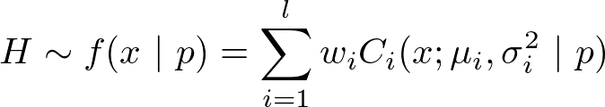
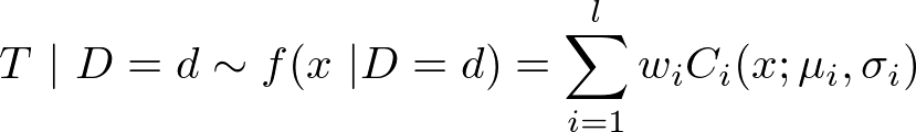
where p is the activity purpose, l the number of components, w_i is the weight associated with the component C_i such that w_i ≥ 0 and ∑_i w_i = 1. Every C_i considered here follows a Log-Normal distribution LN(μ_i, σ²) with location parameter μ_i ∈ ℝ and scale parameter σ² ∈ ℝ. For a detailed description of such mixture distributions, see McLachlan and Peel (2004).

3.10

The empirical and fitted distributions are illustrated in Figures 3 and 4. It is important to note that the number of components is determined so that each mixture distribution obtained is statistically similar to the empirical distribution according to the univariate Kolmogorov-Smirnov goodness-of-fit test (Massey 1951) at a 5% significance level.

3.11

The departure time is then randomly drawn according to the appropriate distribution.

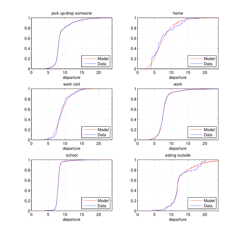
Figure 3. House departure time (hours): empirical and estimated cumulative distribution functions by purpose.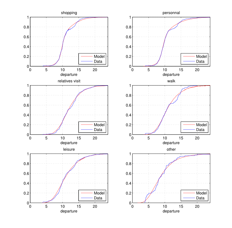

Figure 4. House departure time (hours): empirical and estimated cumulative distribution functions by purpose.

3.12

It should be noted that directly drawing from empirical distribution has also been investigated, but this was up to three times slower in the experiments conducted. As a very large number of draws is involved (in the hundreds of millions), random number generation speed becomes an essential problem to be addressed so this approach has been discarded.

Activity localization

3.13

We now turn to the description of how the localization of an activity is determined inside the Belgian road network. Given that each individual has a house, it is possible to localize each of his/her activities in the network, the house being the starting point of the activity chain. These activities will also take place at a node of the network, which is determined as follows:

1. a distance d is drawn from a distribution pertaining to the considered activity;
2. a set of nodes at distance d from the current localization is generated;
3. finally a node is drawn from the set generated at the previous step.

We provide more details on these three steps in the following subsections.

Random draw of a distance

3.14

Similar to the house departure time, the random draw of the distance d travelled to perform an activity follows a mixture of distribution conditional to the type of the activity chain which is fitted to the empirical distribution obtained from the Mobel survey. Empirical and resulting fitted probability density functions are illustrated in Figures 5 and 6. Again, the distributions do not vary by residential municipality type which can be a limitation of the current implementation.

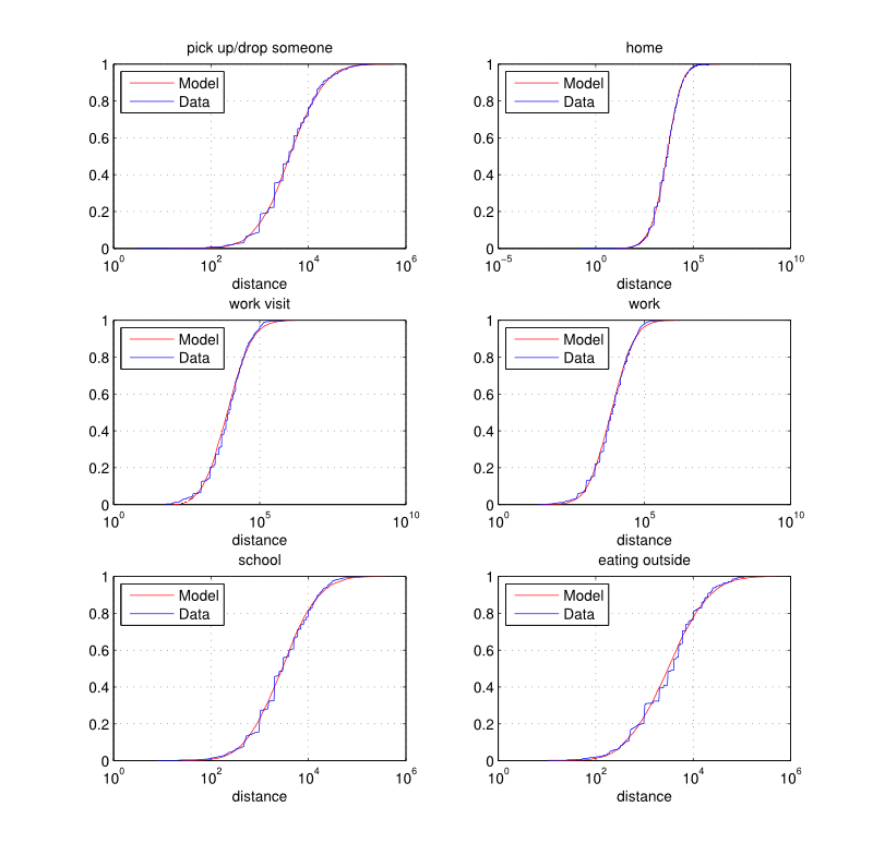
Figure 5. Distance (meters): empirical and estimated cumulative distribution functions by activity type.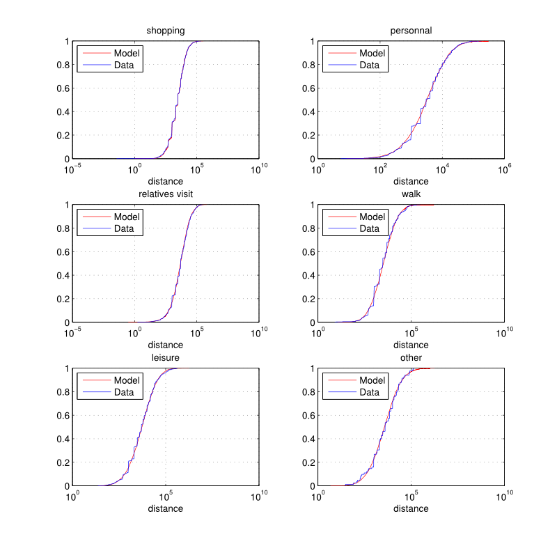

Figure 6. Distance (meters): empirical and estimated cumulative distribution functions by activity type.

Generation of a set of feasible nodes for a given activity

3.15

The next step is to generate a set of nodes at distance d from the current localization, at which the considered activity could take place. A Dijkstra algorithm relying on a Fibonacci heap data structure is used to explore the network and find these feasible nodes. For a network with n nodes and m arcs, this algorithmic variant has the crucial advantage in our context of requiring O(n log n + m) operations, instead of O(n²) for a more direct implementation or O((n + m) log n) for an implementation based on a k-ary heap data structure^[1] (Fredman & Tarjan 1987).

3.16

If no suitable node is found at the desired distance, then the same procedure is applied but with a range of distances [d − ε, d + ε]. This error term ε is increased (in practice, doubled with initial value of 250m) until at least one node is discovered.

Activity node choice

3.17

If no additional data is available, the destination node α^l is then randomly chosen from a discrete uniform draw. Otherwise, the draws can be empirically weighted in order to take information on specific activity localization at specific nodes/municipalities (for instance using geo-localization) into account.

3.18

To illustrate our proposal, assume a road network and an activity choice resulting in a set of 4 feasible nodes, whose indicators for 3 types of activity are detailed in Table 5 (nodes 1 and 2 belong to the same municipality). If no indicator is available, such as for leisure, then the line is set to na; work is a municipality-related indicator and school is a node-related indicator used for precise geo-localization of schools.

Table 5: Nodes' indicators.
Indicator	Node 1	Node 2	Node 3	Node 4
work	1000	1000	500	800
school	0	1	0	0
leisure	na	na	na	na

3.19

The proposed technique has the advantage of using localization data whenever available, but also allows for a reasonable alternative if such information be missing.

Activity duration

3.20

An activity duration depends on its starting time, which is obtained by adding the ending time of the previous activity and the trip duration performed to reach the current location. The time spent to carry out an activity is then determined by:

1. drawing a trip duration t to compute a starting time α^s;
2. and drawing an activity duration α^d conditional to α^s.

These two steps are detailed below.

Trip duration and starting time

3.21

It is clear and confirmed by the trip data extracted from Mobel, that a trip duration t is related to its distance d^[2]. This observation leads us to fit a mixture of bivariate distributions to approximate the joint-distribution of (D, T) where T and D are the random variables associated with the duration and the distance of a trip, respectively. The resulting bivariate distribution is defined by:

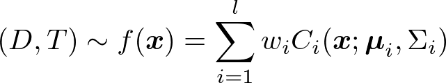
where l is the number of components, w_i is the weight associated with component C_i such that w_i ≥ 0 and ∑_i w_i = 1. The C_i considered here follow a bivariate Log-Normal distribution LN(μ_i, ∑_i) with location vector μ_i = (μ_i,1, μ_i,2) ∈ ℝ² and scale matrix ∑_i = (σ_i,11, σ_i,12; σ_i,21, σ_i,22) ∈ ℝ^2x2.

3.22

As for the distributions of the house departure time and the distance performed to reach an activity, the number of components l is determined in order to obtain a fitted distribution that is statistically similar to the empirical distribution according to Fasano and Franceschini's generalization of the Kolmogorov-Smirnov goodness-of-fit test (Fasano & Franceschini 1987) at the significance level of 5%.

3.23

The fitted distribution is illustrated in Figure 7. As one could expect, there is a positive correlation between the distance and the duration of trip, i.e. the further an individual goes, the more time he/she spends on the road. It can also be noted that the variance of the duration is higher for smaller trips and gradually decreases as the distance increases.

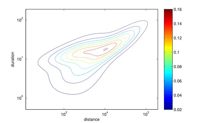
Figure 7. Fitted probability density function of distance (meters) × duration (minutes).

3.24

Since the distance d is computed in a previous step (see Section Random draw of a distance), it follows from (Eaton 1983) that the trip duration t can be drawn from the univariate conditional distribution of T given D = d defined by:

where l is the number of components, w_i are the weights of the mixture and C_i follows a univariate Log-Normal distribution LN(μ_i, σ_i) such that

μi = μi,2 + (σi,12 / σi,12) (d − μi,12)

and

σi = σi,12 − (σi,12)2 / σi,11.

The starting time of α_i ∈ α^* (i > 1) is then obtained by adding the transportation duration and the ending time of the previous activity of the chain, i.e.

αsi = ( αsi−1 + αdi−1) + t.

Activity duration

3.25

Since an activity duration is correlated with its starting time and purpose, the computation of α^d follow a similar process applied for determining a trip duration, i.e. for each purpose the joint-distribution of an activity starting time and its duration is fitted to the data.

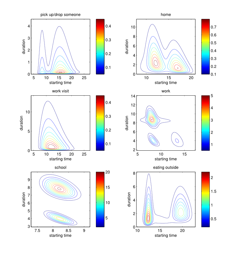
Figure 8. Starting time × Duration (hours): estimated probability density functions by purpose.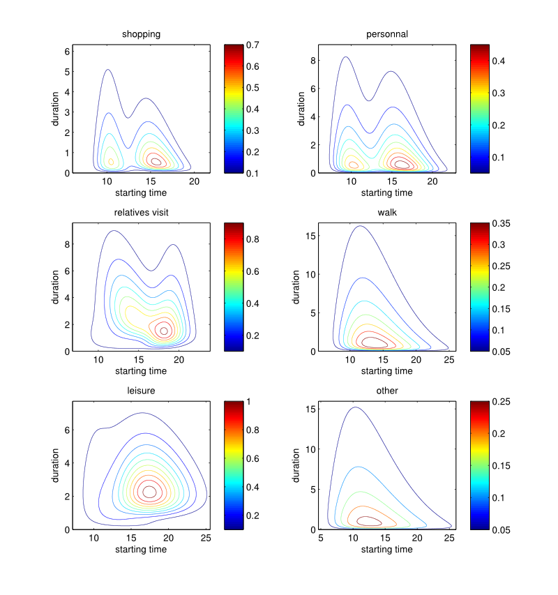

Figure 9. Starting time × Duration (hours): estimated probability density functions by purpose.

3.26

Figures 8 and 9 illustrate the resulting joint-distributions, from which behavioural patterns can be observed. For instance:

• individuals mainly start working at 8:30 for 8 to 9 hours, but the distribution also highlights the part-time worker starting at 8:30 or 13:00;
• students usually start school between 8:00 and 8:30, and remain there either 4 hours (on Wednesday) or 8 hours (the other school days). Also the later a student arrives at school, the less time he spend there;
• eating outside occurs at midday and in the evening. An average midday and evening meal takes 1:20 and 2:15 hours, respectively. This indicates that midday meal duration is more constrained by the time budget available for the remaining activities of the day;
• shopping is mainly done before midday (between 10:00 and 11:00) and around 16:00 i.e. after leaving work, with a typical duration of 30 minutes to 1 hour.

These observations indicate that the fitted distributions produce consistent behaviours.

3.27

A duration α^d is then drawn from the distribution pertaining to the considered activity purpose conditionally to the starting time computed previously.

3.28

Finally, the activity chain of the individual is completed by generating a return to home after the end of the last activity.

Application on VirtualBelgium: results

4.1

Our activity-based model has been successfully applied to the Belgian synthetic population to simulate an average day. As stated in Section 2, the simulation involved 10,300,000 agents spread over 4,350,000 households. With an average of 4.33 activities per individual, we have 43,300,000 activities to characterize. The road network considered is illustrated in Figure 10, which is made of 66,304 nodes and 125,889 links. It is detailed up to the OpenStreetMap tertiary road network.

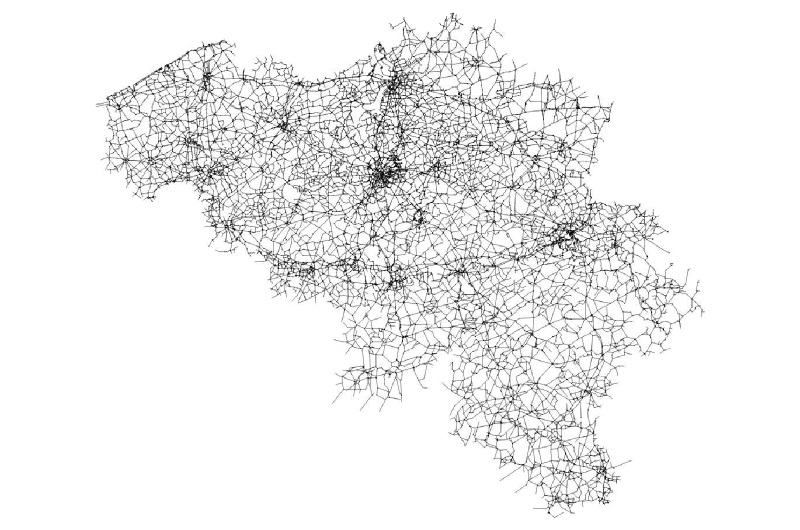
Figure 10. Belgian road network - 66.304 nodes and 125.889 links.

4.2

The sheer size of the simulation generates a substantial amount of computation, making its efficient organization and structure truly challenging. The main computational burden is the execution of many shortest-path calculations for activity localization, as well as efficient random draws. After several preliminary attempts, our current best execution time is approximatively 8:30 hours using 500 Intel Xeon X5650 processor cores and 512MB of RAM per core, a speed up of a factor 50 on our initial implementation. Figure 11 illustrates the high scalability of the simulator running on a cluster of AMD Opteron 4310EE processors. The exploitation of multiple computational cores appears to be efficient, as the observed speed-up is close to the expected theoretical ones, i.e. doubling the number of cores nearly halves the execution time.

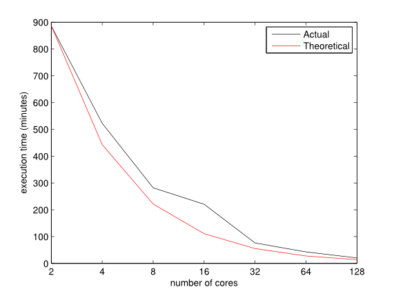
Figure 11. Computation times for 105.250 agents with respect to the number of computational cores.

4.3

The main output of VirtualBelgium consists of a standard XML file describing the agenda of every agent of the simulation. Listing 1 illustrates the agenda of an agent.

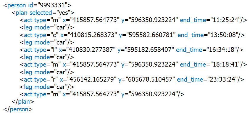
Listing 1. An agent's schedule (XML).

4.4

Figure 12 shows the histogram of proportion of activities starting at each hour of the day. One can easily observe the morning and evening peaks occurring at 8:00 and 16:00, respectively. The comparison for the cumulative distribution function and the probability density function, between the Mobel data and VirtualBelgium are given in Figures 13 and 14. The Kolmogorov-Smirnov test indicates that these distributions are not significantly different. The minor differences may result from correlation structures not taken into account, which implies that the agents can then accumulate delays over the day. This result is crucial since it shows that, at an aggregate level, the VirtualBelgium agents behave as expected.

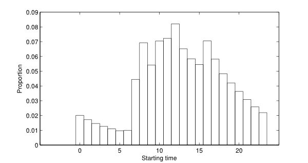
Figure 12. Histogram of the number of activities starting at each hour of the day.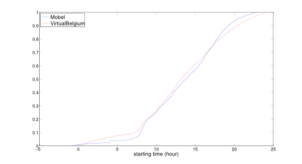

Figure 13. Comparison of the empirical and resulting cumulative distributions for activities' starting time.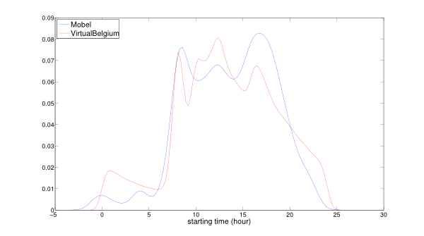

Figure 14. Comparison of the empirical and resulting probability density functions for activity starting time.

4.5

The difference between VirtualBelgium and Mobel in proportion of activity is presented in Figure 15. One can easily see that the differences remain very small, with a maximum difference less than 4%. This observation can validate the generation of activity chain patterns by individual type and the assignment process.

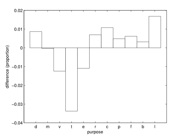
Figure 15. Difference of activity type proportions between VirtualBelgium and Mobel.

4.6

As a micro-simulation model, it is possible to extract results for any sub-section of the population. For instance, we can compare some characteristics of the agents' mobility behaviour with respect to their socio-professional status (active/inactive/student):

• in Figure 16, it can be observed the vast majority of work-related and school activities are performed by active individuals and student as expected. The students tend to have more leisure activities than the other groups. On the other hand, inactive people seem more inclined to shop, stay at home as well as drop/pick up others than the rest of the population.
• Figure 17 illustrates the starting time of the first activity per agent type using a box plot representation. This result highlights the fact that the inactive people start their activities later. A one-way ANOVA also confirmed that (at a 5% significance level) the average starting time of an inactive individual is significantly later than the ones associated with the other groups. This is probably caused by the lack of constraints related to work and school activities.

4.7

These observations show that socio-professional status does affect mobility behaviour. Hence the new methodology seems to produce consistent results. Nevertheless, validating the results for disaggregate levels requires significant data detailing these levels that is unfortunately not available in our context.

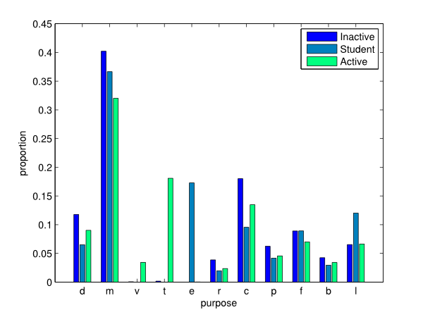
Figure 16. Activity type proportions by socio-professional status.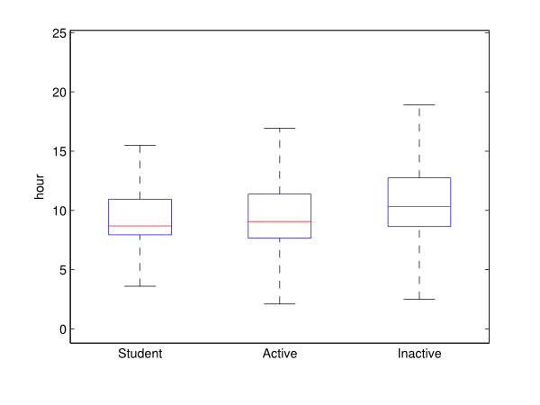

Figure 17. Box plot of the first activity starting time by socio-professional status.

4.8

An interesting output of the model is the origin-destination matrix that identifies the number of trips between municipalities. The total flows for one average day is represented in Figure 18. As expected, the main cities of Belgium attract most of the traffic flows. This can also be observed in the map in Figure 19 which illustrates the number of activities starting between 8:00 and 9:00 of an average day by municipality.

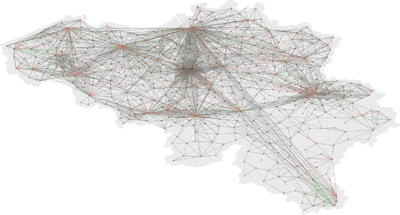
Figure 18. Flows between municipalities. Each represented link corresponds to a minimum of 500 trips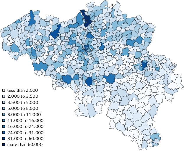

Figure 19. Number of starting activities by municipality between 8:00 and 9:00.

4.9

This result is encouraging as no node indicator (as defined in Section Activity node choice) has been used. This is certainly explained by the fact that these cities have a denser road network (and therefore have more nodes than smaller cities), thus the activity localization process naturally favours them.

4.10

Finally, as the XML output of VirtualBelgium is compatible with MATSim, it is possible to use it to perform dynamic traffic assignment. For instance, Figure 20 illustrates a snapshot of the beginning of the morning peak on the Namur city road network. It is nevertheless important to note that every agent uses the same transport mode, namely the car, as no mode choice model is currently available in VirtualBelgium.

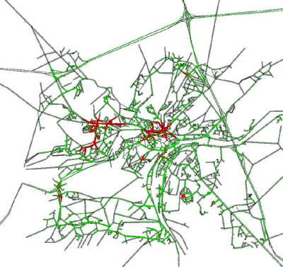
Figure 20. Snapshot of MATSim output. Red agents are stuck in a traffic jam.

Discussion

5.1

Unsurprisingly, the proposed model still requires improvement in order to increase the quality and the reliability of the results. One of the important problems in the current implementation is the lack of a true mode choice for reaching an activity (public transportation, carpooling, walking, etc.).

5.2

It is also clear that the home location of an individual influences the activities he/she may take part in. Indeed, individuals living in villages might present mobility behaviours different from the ones observed in cities or suburbs. Provided that significant data is available, this heterogeneity can be represented by refining the activity chain assignment process as well as the distributions used to characterize the activities by taking into account residential municipality type.

5.3

The current model does not rely on geo-localized data for determining the destinations of the trips performed by the agents and this may introduce a deviation from the true mobility behaviour of the simulated population. Nevertheless, this issue can easily be solved because the approach is designed to easily take advantage of any additional data sources available such as land use and precise geo-localization of dwelling units, schools and shopping centres, job and service indicators by municipality, etc. used by the existing activity based models. The activity location process can then exploit this additional data to weight or constrain the random draws of activity and household home locations to specific nodes in order to provide a better distribution of location than the uniform distribution. For this reason, determining the node indicator values for destination choice (job and service indicators by municipality, school localization, land use, etc.) will need to be investigated.

5.4

Finally, improving the quality of the baseline synthetic population by considering new attributes such as income and employment type might also lead to more accurate simulated mobility behaviour.

Conclusions

6.1

This paper detailed a flexible activity-based model implemented in VirtualBelgium, a micro-simulation platform designed to replicate the evolution of a (Belgian) population and its mobility behaviour. In order to focus only on the modelling of the transportation demand, the framework is compatible with MATSim, a powerful, validated and widely used micro-simulator for traffic assignment.

6.2

The proposed activity-based model is data driven and requires no a priori information about the localization of activities, which means that much less data is required than that required by existing approaches (e.g. ALBATROSS, ILUTE, SAMS, AMOS, etc.). Indeed the minimal requirements of the methodology are:

1. a disaggregate data set representing the population of interest;
2. a set of observed activity chains performed by the individuals;
3. statistical distributions detailing each activity type;
4. and a road network description.

6.3

The first requirement can be either extracted from a census or a synthetic population generated for the area of interest. The second and the third can usually be derived from any mobility survey. Finally the road network can be downloaded (for instance) from the OpenStreetMap project. Hence this new methodology is easily transferable to different study areas/countries. It can also easily take advantage of any additional geo-referenced data to improve the accuracy of the results.

6.4

This work demonstrates that assigning and fully characterizing (temporally and spatially) a sequence of activities to more than 10.000.000 agents is nowadays feasible. Considering the relatively limited amount of input data, the results produced by the new methodology are promising as the synthetic population mobility behaviour is statistically similar to the one observed in the mobility survey.

6.5

Lastly, as VirtualBelgium integrates the detailed model, the (freely available) framework takes a step forward to reproduce and understand the transportation dynamics of a whole country. Future developments of VirtualBelgium thus have the potential for transportation planning by forecasting the evolution of a population and its associated transportation demand. Therefore it enables the design of various (transport) policies to meet future demand and simulate their impacts, for instance on traffic congestion, road safety and environmental issues such as air pollution and energy consumption. This micro-simulator also opens new research perspectives in many different topics where knowing the agents' daily agenda is important. These include such areas as opinion and disease propagation, social network dynamics, socio-demographic evolution of a population, residential mobility, family and social dynamics, etc.

Acknowledgements

The authors wish to thank Frédéric Wautelet and François Damien for their help in setting up the simulation on a high performance computing facility. Computational resources have been provided by the Consortium des Equipements de Calcul Intensif (CECI), funded by the Fonds de la Recherche Scientifique de Belgique (F.R.S.-FNRS) under Grant No. 2.5020.11. Helpful corrections from Eric Cornelis, Véronique Evrard, Laurie Hollaert, Marie Moriamé, Nagesh Shukla and Nam Huynh are also gratefully acknowledged. The authors wish to gratefully acknowledge the help of Dr. Madeleine Strong Cincotta in the final language editing of this paper.

Notes

¹ This computational advantage was confirmed in the experiments conducted as the Fibonacci heap data structure was up to 50× faster than the other ones.

² This fact can easily be graphically represented with a scatter plot of the two attributes.

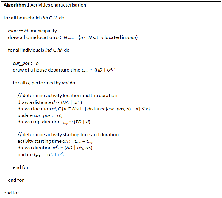
Appendix: Pseudo-code for activity chains characterization

Assuming that every individual agent is provided with a sequence of activity purposes (α^p_i)_{i ∈ {1,...,k}}, the following pseudo-code illustrates how to fully determine each activity α_i = (α^p, α^l, α^s, α^d) performed by the agents. This algorithm requires a synthetic population P = (I , H), a road network G = (N, L), an error term ε ≥ 0 and the following distributions: house departure times HD, distances to next activity DA, trip durations TD and activity durations AD.

References

ADLER, T. & Ben-Akiva M. (1979). A theoretical and empirical model of trip chaining behavior. Transportation Research B, 13(3), 477–500. [doi:10.1016/0191-2615(79)90016-X]

ARENTZE, T. A. & Timmermans, H. J. P. (2000). Albatross: A learning-based transportation oriented simulation system. Technical report, European Institute of Retailing and Services Studies. Eindhoven, The Netherlands.

AVERY, L. (2011). National Travel Survey: 2010. National Travel Survey. Department for Transport.

BARTHELEMY, J. (2014). A parallelized micro-simulation platform for population and mobility behaviour -Application to Belgium. PhD thesis, University of Namur.

BARTHELEMY, J. & Toint, Ph. L. (2013). Synthetic population generation without a sample. Transportation Science, 47(2), 266–279. [doi:10.1287/trsc.1120.0408]

BHAT, C. R. & Koppelman, F. S. (1999). Activity-based modeling of travel demand. In R. W. Hall (Ed.), Handbook of Transportation Science (pp. 35–61), Dordrecht: Kluwer Academic Publishers.

BHAT, C. R., Guo, J. Y., Srinivasan, A. & Sivakumar, A. (2004). Comprehensive Econometric Microsimulator for Daily Activity-Travel Patterns. Transportation Research Record, 1894, 57–66. [doi:10.3141/1894-07]

BRADLEY, M., Bowman, J. L. & Griesenbeck, B. (2010). SACSIM: An applied activity-based model system with fine-level spatial and temporal resolution. Journal of Choice Modelling, 3(1), 5–31. [doi:10.1016/S1755-5345(13)70027-7]

CHAPIN, F. S. (1974). Human activity patterns in the city: Thing people do in time and space. New York: J. Wiley and Sons.

COLLIER, N.T. & North, M. (2012). Parallel agent-based simulation with Repast for high performance computing. SIMULATION. November 6.

CORNELIS, E., Hubert, M., Huynen, Ph., Lebrun, K., Patriarche, G., De Witte A., Creemers, L., Declercq, K., Janseens, D., Castaigne, M., Hollaert, L. & Walle F. (2012). La mobilité en belgique en 2010 : résultats de l'enquête BELDAM. FUSL.

DICKEY, J. W. (1983). Metropolitan Transportation Planning. New York: McGraw-Hill.

DOMENCICH, T. & McFadden, D. (1975). Urban Travel Demand: A Behavioural Analysis. North-Holland Publishing Co.

EATON, M. L. (1983). Multivariate statistics: a vector space approach, (pp. 116-117). M. L. Eaton (Ed.). New York: Wiley.

FASANO, G. & Franceschini, A. (1987). A multidimensional version of the Kolmogorov-Smirnov test. Monthly Notices of the Royal Astronomical Society, 225, 155–170. [doi:10.1093/mnras/225.1.155]

FREDMAN, M. L. & Tarjan, R. E. (1987). Fibonacci heaps and their uses in improved network optimization algorithms. Journal of the ACM (JACM), 34(3), 596–615. [doi:10.1145/28869.28874]

GAN, L. P. & Recker, W. (2008). A mathematical programming formulation of the household activity rescheduling problem. Transportation Research Part B: Methodological, 42(6), 571–606. [doi:10.1016/j.trb.2007.11.004]

GOLOB, T. F. (2003). Structural equation modeling for travel behavior research. Transportation Research Part B: Methodological, 37(1), 1–25. [doi:10.1016/S0191-2615(01)00046-7]

GORAN, J. (2001). Activity based travel demand modeling - A literature Study. Technical Report, Danmarks Transport-Forskning.

HÄGERSTRAND, T. (1970). What about people in regional science?. Papers of the Regional Science, 24(1), 6–21. [doi:10.1007/BF01936872]

HAKLAY, M. M. & Weber, P. (2008). Openstreetmap: User-generated street maps. Pervasive Computing, IEEE, 7(4), 12–18. [doi:10.1109/MPRV.2008.80]

HERMES, K. & Poulsen, M. (2003). A review of current methods to generate synthetic spatial microdata using reweighting and future directions. Computers, Environment and Urban Systems, 36(4), 281–290. [doi:10.1016/j.compenvurbsys.2012.03.005]

HOE, S. L. (2008). Issues and procedures in adopting structural equation modeling technique. Journal of Applied quantitative methods, 3(1), 76–83.

HUBERT, J.-P, & Toint, Ph. L. (2002). La mobilité quotidienne des Belges (No 1). Presses Universitaires de Namur.

KITAMURA, R., Chen, C. & Pendyala, R. M. (1997). Generation of synthetic daily activity-travel patterns. Transportation Research Record, 1607, 154–162. [doi:10.3141/1607-21]

KITAMURA, R., Pas, E., Lula, C., Lawton, T. K. & Benson, P. (1996). The sequenced activity mobility simulator (SAMS): an integrated approach to modelling transportation, land use and air quality. Transportation, 23(3), 267–291. [doi:10.1007/BF00165705]

MASSEY, F. J. (1951). The Kolmogorov-Smirnov test for goodness of fit. Journal of the American Statistical Association, 46(253), 68–78, 1951. [doi:10.1080/01621459.1951.10500769]

MCLACHLAN, G. & Peel, D. (2004). Finite Mixture Models. J. Wiley and Sons.

MEISTER, K., Balmer, M., Ciari, F., Horni, A., Rieser, M., Waraich, R. A. & Axhausen, K. W. (2010). Large-scale agent-based travel demand optimization applied to Switzerland, including mode choice, paper presented at the 12th World Conference on Transportation Research, July 2010.

MILLER, E. (1997). Microsimulation and activity-based forecasting. In Activity-Based Travel Forecasting Conference.

NAGEL, K., Beckman, R. L. & Barrett, C. L. (1999). Transims for transportation planning. In 6th Int. Conf. on Computers in Urban Planning and Urban Management.

OPPENHEIM, N. (1995). Urban Travel: From Individual Choices to General Equilibrium. New York: J. Wiley and Sons.

SALVINI, P. & Miller, E. J. (2005). Ilute: An operational prototype of a comprehensive microsimulation model of urban systems. Networks and Spatial Economics, 5, 217–234. [doi:10.1007/s11067-005-2630-5]

SPEAR, B.D. (1977). Application of new travel demand forecasting techniques to transportation planning: a study of individual choice models (No. FHWA/PL-77012).

TANTON, R. (2014). A review of spatial microsimulation methods. International Journal of Microsimulation, 7(1), 4–25.

TANTON, R. & Edwards, K. (Eds.). (2012) Spatial Microsimulation: A Reference Guide for Users (Vol 6). Springer.

VAN DAM, K. H. , Nikolic, I. & Lukszo, Z. (2012). Agent-based Modelling of Socio-technical Systems (Vol. 9). Springer.

WADDELL, P. (2002). Urbansim: Modeling Urban Development for Land Use, Transportation and Environmental Planning. Journal of the American Planning Association, 3(3), 297–314. [doi:10.1080/01944360208976274]