Abstract

The Schelling model is a simple agent-based model that demonstrates how individuals’ relocation decisions can generate residential segregation in cities. Agents belong to one of two groups and occupy cells of rectangular space. Agents react to the fraction of agents of their own group within the neighborhood around their cell. Agents stay put when this fraction is above a given tolerance threshold but seek a new location if the fraction is below the threshold. The model is well-known for its tipping point behavior: an initially random (integrated) pattern remains integrated when the tolerance threshold is below 1/3 but becomes segregated when the tolerance threshold is above 1/3. In this paper, we demonstrate that the variety of the Schelling model’s steady patterns is richer than the segregation–integration dichotomy and contains patterns that consist of segregated patches of each of the two groups, alongside areas where both groups are spatially integrated. We obtain such patterns by considering a general version of the model in which the mechanisms of the agents' interactions remain the same, but the tolerance threshold varies between the agents of both groups. We show that the model produces patterns of mixed integration and segregation when the tolerance threshold of an essential fraction of agents is either low, below 1/5, or high, above 2/3. The emerging mixed patterns are relatively insensitive to the model’s other parameters.

Keywords:

Schelling Model, Ethnic Segregation, Residential Dynamics, Heterogeneous Agents

Introduction

1.1

The Schelling model of segregation was introduced by Thomas Schelling in the late 1960s (Schelling 1969, 1971, 1974, 1978). Schelling devised the model in order to demonstrate how individuals' relocation decisions entail global segregation. Schelling noted that his abstract model could reflect different spatial phenomena, but his main concern was the residential segregation of blacks and whites in United States cities (Schelling 1969, p. 488). In this interpretation, the model consists of households that make residential decisions based on the ethnic composition of neighborhoods.

1.2

Using today's terminology, the Schelling model is an agent-based model. Agents belong to one of two groups and are located in the cells of rectangular space. A cell can be either empty or occupied by a single agent. Agents react to the fraction \(f\) of friends (i.e. agents of their own group) in the local neighborhood of a cell. An agent is satisfied with its location when the fraction of friends in the cell's neighborhood is equal or above the threshold \(F\), \(f \geq F\). However, when the fraction of friends in the neighborhood is below \(F(f < F)\), an agent tries to relocate to an empty cell for which the fraction of friends in the neighborhood is satisfactory (\(f \geq F\)). The minimum fraction of friends \(F\) required by an agent to be satisfied is known as the tolerance threshold.

1.3

A wide spectrum of formal representations of the Schelling mechanism exhibits various aspects of a well-known tipping point behavior: An initially random pattern remains, in time, integrated for \(F < F_{\rm critical}\), while it converges to segregation for \(F \geq F_{\rm critical}\). The tipping point \(F_{\rm critical}\) is about 1/3, indicating that a relatively weak individual tendency to segregate is sufficient for global segregation. Based on this result Schelling argued that residential segregation in cities could form even when all of the individuals are willing to live within integrated neighborhoods, and no ethnic discriminatory mechanism or economically-induced segregation exist (Schelling 1971).

1.4

Schelling's mechanism of residential relocation constitutes the core of comprehensive models of real-world residential dynamics (Ellis et al. 2012). It is thus important to investigate whether the segregation-integration dichotomy is the only possible outcome of the Schelling model. In this paper, we demonstrate that the model's repertoire is not limited to merely integration (Figure 1a) or segregation (Figure 1b), but also includes intermediate patterns that simultaneously contain segregated and integrated parts (Figure 1c). Below, we refer to these patterns that contain segregated patches for each population group as well as patches where both groups coexist as mixed patterns.

Figure 1. Steady residential patterns of blue and green agents. The Ic and C indices are introduced in Section 6 below.

1.5

Our research provides an extension of the Schelling model that accounts for the heterogeneity that exists in real world populations. As we demonstrate, mixed patterns emerge in the Schelling model when agents' tolerance thresholds vary among the members of the same group. Namely, when an essential fraction of the agents of both groups has either a low tolerance threshold (tolerant agents) or a high tolerance threshold (intolerant agents). We consider various distributions of tolerance threshold and reveal the conditions for the emergence of mixed patterns.

1.6

The paper has the following structure: Section 2 demonstrates the relevance of mixed patterns to the spatial ethnic patterns of cities. Section 3 presents a brief review of the Schelling model studies. Section 4 presents the model formally and Section 5 describes the tolerance distributions used in the study. The indices that are exploited for characterizing residential patterns are introduced in Section 6, followed by the results in Section 7. We summarize our findings in Section 8.

Urban patterns of ethnicity

2.1

Our interest in mixed patterns is not purely theoretical. Besides the intent of broadening our understanding of the Schelling model behavior, we are motivated by the ethnic patterns in real-world cities that are not purely integrated and segregated, but contain both integrated and segregated neighborhoods. The latter, according to the 2010 US census, is characteristic for many US cities where, despite some decline since 1970s (Glaeser & Vigdor 2012), ethnic segregation is still prevalent (Logan & Stults 2011). A visual assessment of the ethnic residential patterns of cities uncovers intricate patterns of segregation and integration, which are similar to the aforementioned mixed patterns. Maps in Figure 2 present examples of Chicago and New York and show fractions of Black, Hispanic, White, and Asian populations, alongside the Shannon entropy index (Arndt 2004) calculated on these fractions^[1]. To recall, a low value of the Shannon entropy manifests homogeneity of the area, whereas a high value is charactersitic of an area where several population groups coexist.

Figure 2. The fraction of Black, Hispanic, White, and Asian adults within the census blocks in 2010, and the Shannon entropy index for Chicago and New York. The legend is valid for both population fractions and the Shannon entropy index.

2.2

The Chicago residential pattern contains large segregated areas of Black, Hispanic, and White populations, and a small segregated area of Asian population (Figure 2a). However, according to the entropy map that depicts areas populated by a variety of ethnic groups, not all areas are segregated. These include Rogers Park, West Ridge, Edgewater, and Uptown in the north (marked A), Bridgeport (marked B) and Hyde Park (marked C).

2.3

New York is less segregated than Chicago (Figure 2b). Examples of ethnically diverse neighborhoods in New York are Richmond Hill, Woodhaven, and Ozone Park in Queens (marked D); while East Flatbush and Remsen Village in Brooklyn (marked E) are segregated. Ethnic patterns that are composed of mixed integration and segregation exist in many other US and Israeli cities (Hatna & Benenson 2012).

The Schelling model

3.1. Schelling's original studies

3.1

Schelling introduced the initial version of the model in 1969 (Schelling 1969). He referred to it as linear because it considered a one-dimensional array of resident locations. All array cells are populated by "stars" ("+") and "zeros" ("0") representing agents of two groups. An agent is dissatisfied with its location when the fraction of friends in the eight nearest cells, four at each side, is below the tolerance threshold. The dissatisfied agent relocates to the nearest position where the fraction of friends is above the threshold. Because all cells are occupied, a migrating agent is inserted into its new position and other agents are shifted aside. The model is updated at discrete time steps, one agent at a time, in a predefined order. With the linear model, Schelling illustrated that for \(F = 0.5\), an initially random pattern converges to a segregated pattern that consists of long sequence of stars and zeroes.

3.2

In a later publication Schelling (1971) presented a two-dimensional version of the model, where agents are not shifted sideways in order to make room for relocating agents. Instead, Schelling introduced empty cells as potential destinations for relocating agents. In a 2D version, agents dissatisfied with their local 3-by-3 neighborhood move to the nearest empty cell that has a sufficient fraction of friends. Here, Schelling revealed for the first time that the value of \(F_{\rm critical}\) that separates segregation and integration is essentially below the intuitive value of 1/2 and close to 1/3. That is, for \(F < 1/3\), an initially random residential pattern remains random-like; while for \(F \geq 1/3\), the pattern converges to a state of global segregation (Schelling 1971, p158).

3.2. Later studies

3.3

The body of literature on the Schelling model accumulated since the 1970s is far too large and fragmented to allow for a comprehensive review within this paper. We thus consider several relevant publications only.

3.4

Benenson and Hatna (2011) were the first to reveal that the Schelling model can generate patterns where integration and segregation co-exist. More specifically, they demonstrated that when two groups are of different sizes and \(F < F_{\rm critical}\), the model produces a segregated patch for the majority group while the rest of the area is occupied by both groups. In a later study, Hatna and Benenson (2012) showed that the model generates similar patterns when the tolerance thresholds are group-specific and the tolerance threshold of one group is between \(F_{\rm critical}\), and 0.5, while the tolerance threshold of the second group is below \(F_{\rm critical}\).

3.5

Xie and Zihaou (2012) were the first to study a Schelling model where each agent holds a personal preference concerning the ethnic composition of neighborhoods. They based the agents' tolerance regarding neighborhood composition on a US survey that revealed large heterogeneity in whites' tolerance for black neighbors and extended the model of Bruch and Mare (2006, 2009) where all white and black agents have the same utility functions. The Xie and Zihaou (2012) model generates a lower level of racial residential segregation when compared to the case where all agents have the same racial tolerance, but the authors did not indicate whether the model produces patterns of mixed integration and segregation.

3.6

Vinkovic and Kirman (2006) provide a general insight into the relation between rules and patterns by considering a continuous analog of the Schelling model. They distinguish between the relocation rules that enable relocation to a better location only and the rules that enable relocation to a cell of the same utility. The rules of the first type generate patterns that stall with an essential fraction of discontent agents who are unable to find a better location. The rules of the second type generate patterns that do not stall, even when all agents are satisfied. In time, patterns in this model converge to stochastic equilibrium in which their statistical characteristics, such as level of segregation, slightly fluctuate around the long-term average.

3.7

Vinkovic and Kirman (2006) demonstrate that the patterns are very sensitive to parameters when the rules allow for relocation to better cells only. For example, the size of the homogeneous clusters depends on the fraction of unoccupied cells. In contrast, when the agents are able to relocate to cells of the same utility, the model patterns are far less sensitive to the model settings. For example, all steady segregated patterns consist of two clusters, one for each group.

3.8

In this study, based on Vinkovic and Kirman's (2006) results, we set rules allowing an agent to relocate between cells of the same utility. We consider this feature as a reflection of the reasons for human migration that are unrelated to the ethnic composition of the neighborhood. At the same time, we restrict this kind of migration in the model to satisfied agents; dissatisfied agents migrate to better locations only.

Model rules

4.1

The rules of the model that are used in this study follow Hatna and Benenson (2012). Urban space is represented by a \(N \times N\) array of cells on a torus. A cell is either vacant or populated by a single agent. We denote an agent as \(a\), a cell as \(c\), and the Moore \(n \times n\) neighborhood of \(c\), excluding \(c\) itself, as \(U(c)\). Each agent \(a\) belongs to one of two color groups: blue or green, and has a personal tolerance threshold \(F_a\). An agent considers other agents of the same color as belonging to its own group; we refer to them as friends. Agent \(a\) is always aware of the fraction of friends \(f_a(c)\), excluding itself, among the agents located in \(U(c)\); this estimate ignores vacant cells of \(U(c)\).

4.2

Agent \(a\) evaluates the utility \(u_a(c)\) of a cell \(c\) within a non-empty neighborhood according to the fraction of friends within the \(U(c)\) and \(a\)'s tolerance threshold \(F_a\):

$$ \begin{array}{ll} u_a(c) = \min\{f_a(c), F_a\}/F_a & \mathrm{if~} F_a > 0\\ u_a(c) = 1 & \mathrm{if~} F_a = 0\\ \end{array} $$

(1)

The utility of a cell in an empty neighborhood is defined as 0. According to (1), the utility varies on [0, 1] (Figure 3).

4.3

The agent is satisfied with a cell \(c\) if \(u_a(c) = 1\) that is, the fraction of friends within neighborhood \(U(c)\) is \(F_a\) or higher. That is, in the case of \(f_a(c) < F_a\) the more friends the better, while for \(f_a(c) \geq F_a\) the number of friends is not important.

Figure 3. An example of the utility function for an agent with a personal tolerance threshold \(F_a = 0.5\). This agent is satisfied when 50% or more of its neighbors are of the same color.

4.4

Time in the model is discrete. At every time step, each agent makes relocation decision by taking the following steps:

Step 1: Agent \(a\) located in cell \(h\) decides whether to relocate:

• \(a\) Generates a random number \(p\), uniformly distributed on \([0, 1)\).
• If \(u_a(h) < 1\) or (\(u_a(h) = 1\) and \(p < m\)), then \(a\) tries to relocate, otherwise \(a\) decides to stay at \(h\). That is, the dissatisfied agent constantly tries to relocate, while the satisfied agent tries to relocate with probability \(m\).

Step 2: If agent \(a\) decides to relocate, then it searches for a new location. The agent compares the utility of its current cell to a set of unoccupied cells and decides whether to move:

• \(a\) Randomly selects \(w\) unoccupied cells from all cells that are unoccupied at that moment, \(V_a\).
• \(a\) Estimates utility \(u_a(v)\) of each vacant cell \(v \in V_a\) and selects the one with the highest utility \(u_a(v_{\rm best})\). If there are several equally best vacancies in \(V_a\), \(a\) chooses one of them randomly.
• \(a\) Moves to \(v_{\rm best}\) if either of the following two conditions are met (otherwise it stays at \(h\)).
• \(u_a(h) > 1\) and \(u_a(v_{\rm best}) > u_a(h)\), i.e., \(a\) is dissatisfied with its current cell \(h\) and \(v_{\rm best}\) is better than \(h\).
• \(u_a(h) =1\) and \(u_a(v_{\rm best} = 1\), i.e., \(a\) is satisfied with \(h\) but moves to \(v_{\rm best}\) which is also satisfactory.

4.5

At every time step, each agent performs the above sequence of decisions once. Following Schelling's original approach, we use asynchronous updating (Cornforth et al. 2005) and allow each agent to make its decision based on the instantaneous state of the pattern. Agents are processed in random order, which is established anew at each time step.

4.6

Our model rules differ from Schelling's description in the following respects:

• A satisfied agent tries to relocate with the nonzero probability \(m\). Schelling's assumption is \(m = 0\).
• The distance between cells has no effect on agents' relocation. In Schelling's model, agents move to the closest satisfactory position.
• Agents can move from one unsatisfactory cell to another if the utility of the new location is higher than that of the previous one. In Schelling's description, agents only move to satisfactory cells^[2].

Model Investigation

Tolerance thresholds of agents

5.1

We explore different distributions of agents' tolerance thresholds, but limit our investigation to the symmetric case of identical distribution within each color group. We start with the simple case where all agents share the same tolerance threshold and then examine tolerance distributions of two kinds:

1. Dichotomous: Blue and green populations consist of two subgroups: The tolerance threshold is \(F_1\) for a fraction \(\alpha\) of agents and \(F_2\) for the rest. This leads to four groups of agents: blue with \(F_1\) tolerance, blue with \(F_2\) tolerance, green with \(F_1\) tolerance and green \(F_2\) tolerance.
2. Beta-binomial: This distribution is sufficiently flexible for generating a variety of tolerance threshold distributions by altering the two shape parameters.

5.2

Besides distribution of tolerance, we explore the influence of the population ratio of blue and green agents on the model pattern. We characterize this ratio by the fraction of blue agents \(\beta\); \(\beta = 0.1\), for instance, indicates that the population consists of 10% blue and 90% green agents. A population with an equal number of blue and green agents is characterized by \(\beta = 0.5\).

5.3

We use a \(5\times5\) Moore neighborhood which results in 181 unique fractions of friends in the neighborhood^[3]. However, we investigate model patterns as dependent on the 25 discrete values of \(F_a\) only, namely of \(F_a = 0/24, 1/24, \ldots, 24/24\) that characterize fully occupied neighborhoods. We limit our study to this set of the \(F_a\)-values because we are interested in residential patterns characteristic of an overall density of agents close to 100%. These selected values of \(F_a\) are sufficient for an adequate portrait of the model behavior in the case of high population density. We use the full set of 181 values in section 7.1.2 to estimate model behavior when the tolerance threshold is close to the tipping point.

General settings

5.4

Unless otherwise stated, we use the following settings in all numeric experiments:

• Grid dimensions: \(50\times50\) cells.
• 98% of the grid is occupied, that is, 50 of 2500 cells are vacant.
• 1:1 ratio of blue and green agents (\(\beta = 0.5\)).
• Agent evaluates \(w = 30\) unoccupied cells per time step when considering relocation.
• Probability of relocation by a satisfied agent \(m = 0.01\).
• Initial agent residential pattern is random.

Evaluation of the model outcomes

6.1

We estimate the long-term behavior of the model by running it for 50,000 time steps. For experiments presented in this study, the model patterns converge during this time interval to a quasi-stable state in which their statistical properties are stable and independent of the initial residential pattern.

6.2

Note that the model's patterns can stall in a state in which some of the agents are dissatisfied with their location but the number of possible relocation options is zero for all agents. For the settings used in this study (section 5.2) and a homogeneous tolerance threshold \(F\) for all agents, the patterns stall at a highly segregated configuration when \(F \geq 14/24\). As we will see below, these situations are of marginal interest for our study.

6.3

The model produces two residential patterns: by color (i.e., blue and green agents) and by agents' tolerance thresholds. To describe these patterns, we exploit three measures proposed in Hatna and Benenson (2012):

Index of color (\(I_{\rm C}\)) and tolerance (\(I_{\rm T}\)) segregation

6.4

The level of segregation of the color and tolerance patterns is measured by the Moran's \(I\) index of spatial association (Anselin 1995). We denote \(I_{\rm C}\) as the index for color and \(I_{\rm T}\) as the index for tolerance segregation. For random (integrated) patterns, \(I\) is close to zero (Figure 1a), while for fully segregated patterns, \(I\) is close to 1 (Figure 1b)^[4]. An intermediate value of \(I_{\rm C}\) implies a moderate level of color segregation, but it does not necessarily indicate the presence of a mixed pattern. In order overcome this limitation of \(I_{\rm C}\), we introduce the \(C\) index.

Identifying mixed patterns (\(C\) index)

6.5

We employ the \(C\) index to identify mixed patterns. This index evaluates how closely a color pattern resembles a pattern with three equal sized green, blue, and integrated regions, as the one shown in Figure 1c. To estimate \(C\), the regions of (1) pure blue, (2) pure green, and (3) integration, and the boundaries between them are recognized (see Hatna & Benenson 2012 for details) (Figure 4). Then \(C\) is estimated as the fraction of the smallest of three regions relative to the size of the entire grid. If one of three regions is not present in the pattern then the value of \(C = 0\).

6.6

Figure 4 depicts the partition of the mixed pattern shown in Figure 1c into the three regions. These regions are of similar size, each taking up about 21% of the total area and the rest of the area is taken by the boundary. That is, \(C = 0.21\). \(C\) is zero for the integrated and segregated patterns in Figures 1a and 1b, as they contain only two of three possible regions. Below, the values of all model indices are averaged over 30 model runs with identical values of parameters.

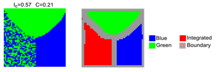
Figure 4. The partition of the mixed pattern shown in Figure 1c into blue, green, and integrated regions, and a boundary.

Results

7.1

We present the results in four sections: In Section 7.1, we describe the simple case where all agents share the same tolerance threshold. In section 7.2, we introduce variability by considering dichotomous tolerance thresholds in order to produce mixed patterns. In Section 7.3, we explore the sensitivity of the mixed patterns to various parameters, and in Section 7.4, we explore cases where the thresholds are distributed across the entire tolerance range using the Beta-binomial family of distributions. Table 1 presents a summary of all investigated cases.

Table 1: A summary of investigated cases, by sub-sections
Section	Investigated case
7.1	All agents share common tolerance threshold \(F\)
7.1.1	Model dynamics in the case of zero probability \(m\) of the random relocation of satisfied agents, \(m = 0\)
7.1.2	The dependence of the tipping point on the probability \(m\) of random relocation of satisfied agents in the case of \(m > 0\)
7.1.3	Dependence of the time of convergence to a steady pattern on the tolerance threshold \(F\) for the value of \(m = 0.01\) (that is chosen for further model studies)
7.1.4	Details of patterns dynamics for the values of \(F\) near and essentially above the tipping point
7.2	Emergence of mixed patterns when half of the agents of each color has tolerance threshold \(F_1\), while the other half has tolerance threshold \(F_2\)
7.2.1	Agents of one subgroup are indifferent to agents of the other group - \(F_1 = 0\), tolerance threshold \(F_2\) of the agents of the second sub-group varies
7.2.2	Tolerance threshold \(F_1\) of the agents of one subgroup is below the tipping point - \(F_1 = 3/24\), tolerance threshold of the agents of the second sub-group \(F_2\) – varies
7.2.3	Tolerance threshold \(F_1\) of the agents of one subgroup is near the tipping point - \(F_1 = 5/24\), tolerance threshold of the agents of the second sub-group \(F_2\) – varies
7.2.4	Tolerance threshold \(F_1\) of the agents of one subgroup is above the tipping point - \(F_1 = 7/24\), tolerance threshold of the agents of the second sub-group \(F_2\) – varies
7.2.5	Complete description of the model patterns' characteristics as dependent on \(F_1\) and \(F_2\)
7.2.6	Detailed study of the mixed pattern dynamics for the representative case of \(F_1 = 3/24\) and \(F_2 = 20/24\)
7.3	Sensitivity of the steady pattern properties to the model parameters when the tolerance threshold is dichotomous
7.3.1	Sensitivity to the fraction \(a\) of \(F_1\) agents
7.3.2	Sensitivity to the fraction \(\beta\) of blue agents
7.3.3	Sensitivity to the probability \(m\) of relocation of satisfied agents
7.3.4	Sensitivity to the neighborhood's size
7.4	Emergence of mixed patterns when the population distribution of the tolerance threshold is Beta-binomial
7.4.1	Study of five qualitatively different beta-binomial tolerance distributions: positively skewed, symmetric, uniform, and two U-shaped
7.4.2	Complete description of the steady model pattern for Beta binomial distribution of tolerance threshold

All agents share the same tolerance threshold \(F\)

7.2

The investigated version of the model incorporates a few features that were not specified in or are different from the features of Schelling's original model as presented in Section 4. The most important of these is the ability of satisfied agents to relocate. To provide a background, we investigate a basic Schelling model in which all agents have the same tolerance threshold \(F\) and demonstrate that the tipping point behavior of our version of the model is the same as that of the original one. Specifically, we demonstrate the dependence of the model's patterns on the probability of relocation by satisfied agents (\(m\)), characterize the time it takes for the patterns to segregate as dependent on \(F\), and demonstrate how patterns converge, in time, to segregation.

\(m = 0\) – Satisfied agents do not move

7.3

For \(m = 0\), the steady pattern is sensitive to the initial one. If the initial pattern is fully segregated, then it remains unchanged for any value of \(F\). If the initial pattern is random (i.e., fully integrated), then it remains random for \(F \leq 7/24\) but converges to segregation for \(F \geq 9/24\). For the intermediate case of \(F = 8/24\), an initially random patterns stalls after some 10 time steps in a partly segregated state, in which dissatisfied agents are not able to improve their location; this stalled residential pattern essentially depends on the details of initial pattern.

The dependence of the tipping point on \(m\) (\(m > 0\))

7.4

For \(m > 0\), the model exhibits a clear tipping point behavior with the tipping value depending on \(m\). In order to gain a detailed description of this dependency, we consider all 181 possible values of \(F\) (Figure 5).

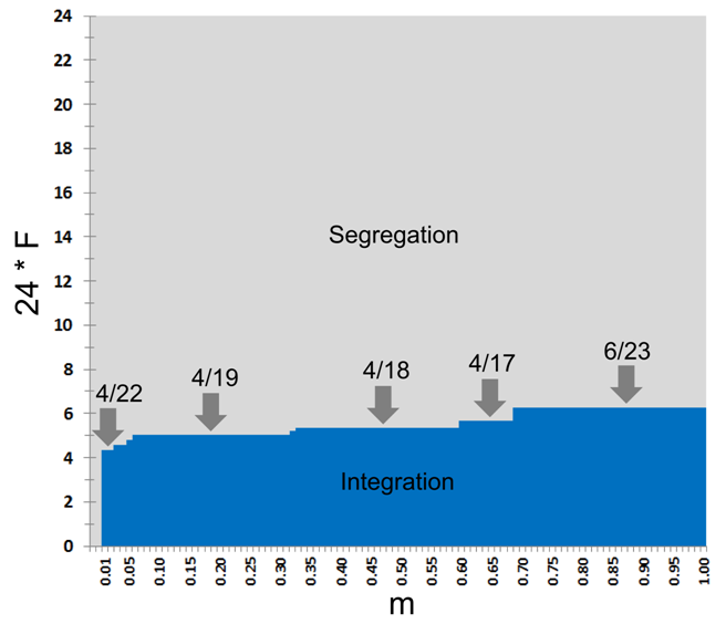
Figure 5. The model's steady patterns as dependent on the tolerance threshold \(F\) and the rate \(m\) of relocation attempts by satisfied agents. The domain of the integrated patterns is marked by blue, while the domain of segregated patterns by grey.

7.5

As can be seen from Figure 5, the value of \(F\) at the tipping point grows with the increase of \(m\). For \(m = 0.01\) the transition between integration and segregation occurs at \(F_{\rm critical} = 4/22 \approx 0.18\), for \(m \in [0.06, 0.31]\) at \(F_{\rm critical} = 4/19 \approx 0.21\), for \(m \in [0.33, 0.57]\) at \(4/18 \approx 0.22\), for \(m \in [0.60, 0.68]\), at \(4/17 \approx 0.23\) and for \(m \in [0.69,1.00]\) at \(F_{\rm critical} = 6/23 \approx 0.26\). The reason for the increase of \(F_{\rm critical}\) with the increase in \(m\) is the growing influence of random migration on the initial clustering of agents^[5].

7.6

In what follows, we investigate the Schelling model for a low value of \(m = 0.01\) and limit our study to 25 values of \(F = 0/24,1/24,\ldots, 24/24\). For this \(m\), \(F = 5/24 \approx 0.20833\) is the minimal tolerance that is above the tipping point of \(F_{\rm critical} = 4/22\). We refer to this value as near the tipping point value.

Dependence of the time of convergence to segregation on \(F\)

7.7

For \(m = 0.01\), an initially random pattern converges to segregation for \(F \geq 5/24\), and the time of convergence depends on \(F\) (Figure 6). As should be expected, the average convergence time and the variation of this time are the highest for the near tipping point value of \(F = 5/24\). For this \(F\) it takes, on average, about 10,000 time steps and varies, in 100 experimental runs performed for the same values of parameters, between 5,000 and 25,000 time steps. Then, with the growth of \(F\), the average convergence time and the variation of this time sharply decrease (Figure 6), and for high tolerance values, such as \(F \geq 12/24\), it always takes four time steps only.

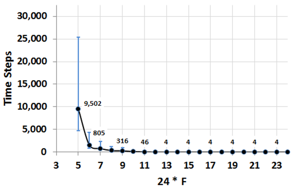
Figure 6. The average and the variation of the number of time steps required to reach a segregated pattern (\(I_C \geq 0.8\)) as dependent on \(F\), based on 100 runs. The value of \(m = 0.01\), blue vertical lines represent 95% confidence intervals.

Details of patterns' dynamics

7.8

Figure 7 shows the dynamics of the color segregation (\(I_C\) index), of the level of mixing \(C\), and the steady model patterns for \(F = 5/24\) and \(F = 7/24\). As can be seen from Figure 7b, the patches of green and blue agents emerge and grow until merging into two large patches, one for each group. Further dynamics result in minimizing the length of the boundary between these two patches. Figure 7 illustrates that the process of convergence is slower for \(F = 5/24\) as compared to \(F = 7/24\).

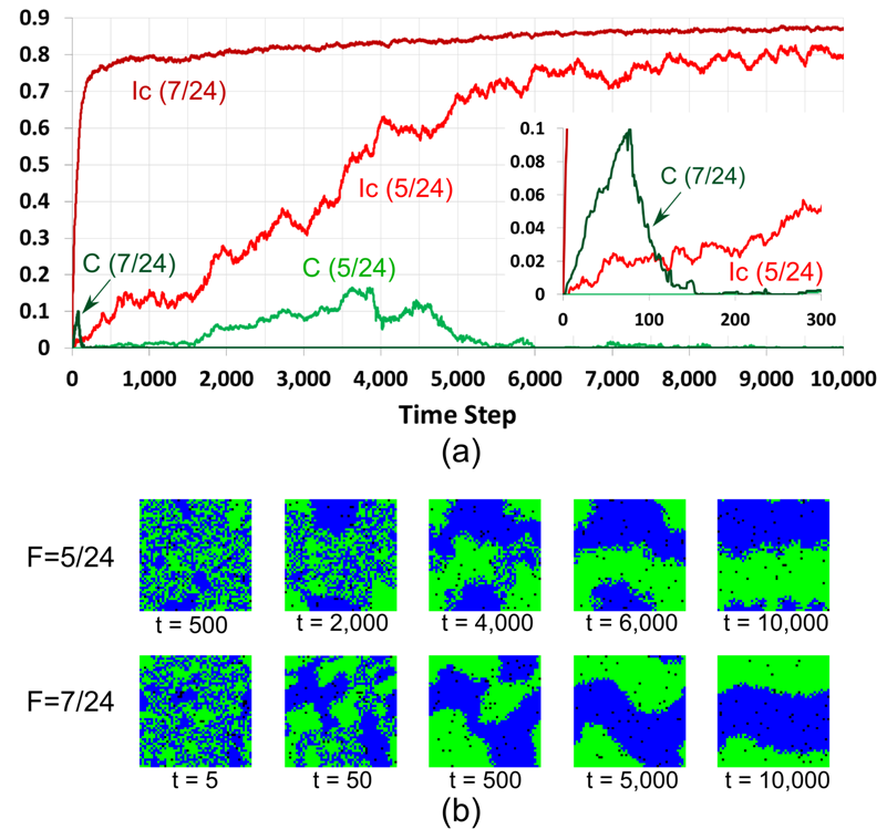
Figure 7. Model runs for \(F = 5/24\) and \(F = 7/24\): (a) dynamics of \(I_C\) and \(C\), the inset graph depicts the first 300 time steps; (b) color patterns at different time steps.

7.9

It is worth noting that during the growth of the blue and green patches, the patterns still contain integrated areas. The patterns are thus mixed, both visually and according to the value of \(C\). Integrated areas dissolve in time as the blue and green agents migrate and segregate throughout the entire pattern.

7.2. Two sub-groups characterized by different tolerance thresholds

7.10

As demonstrated above, the residential pattern of agents whose tolerance threshold is identical, either remains integrated forever or converges to a segregated pattern. Variability of the tolerance thresholds alters this basic result and brings in mixed patterns. We start with the settings in which each color group is composed of two equal sized subgroups: half of blue and green agents have a tolerance threshold \(F_1\), while the other half has a tolerance threshold \(F_2\). According to our definitions of the model parameters in Section 5.1, these settings correspond to the case of \(a = 0.5\). We keep the number of blue and green agents equal as well (\(\beta = 0.5\)).

7.11

In what follows, we fix four values of the tolerance threshold of the first sub-group:

1. Zero, \(F_1 = 0/24\),
2. Below the tipping point \(F_1 = 3/24\),
3. Near tipping point \(F_1 = 5/24\),
4. Above the tipping point \(F_1 = 7/24\).

7.12

For each of these values, we study the details of model dynamics as dependent on \(F_2\). Then we present the general properties of the model patterns for all possible (\(F_1, F_2\)) pairs and conclude the section by demonstrating the temporal development of the mixed patterns. To recall, given a set of model parameters the simulation is repeated 30 times and all pattern characteristics are averaged over these 30 runs. The patterns at \(t = 50{,}000\) are considered as steady.

\(F_1 = 0\), \(F_2\) varies

7.13

When \(F_1 = 0/24\), half of the agents of each color are fully tolerant and are thus satisfied within any neighborhood and only attempt to relocate for random reasons, i.e., at a rate \(m\). Model patterns still depend on the tolerance threshold \(F_2\) of the other half of the agent population. Figure 8a presents the dependence of three measures – \(I_{\rm C}\) of segregation by color, measure \(I_{\rm T}\) of segregation by tolerance threshold, and measure \(C\) of pattern mixing on \(F_2\). For \(F_2 < 5/24\), the pattern is integrated: starting at \(F_2 = 5/24\), the value of \(I_{\rm C}\) grows linearly with \(F_2\) and stabilizes at \(F_2 = 18/24\) at a level of 0.46. Segregation by tolerance, characterized by the value of \(I_{\rm T}\), remains zero for all \(F_2 < 12/24\). For larger values of \(F_2\), \(I_{\rm T}\) grows with the growth of \(F_2\), stabilizing at the value of 0.7 at \(F_2 = 18/24\). According to the \(C\)-measure, for \(F_2 \geq 16/24\), the color pattern is mixed, see steady patterns for \(F_2 = 17/24\) and \(F_2 =20/24\) in Figure 8b.

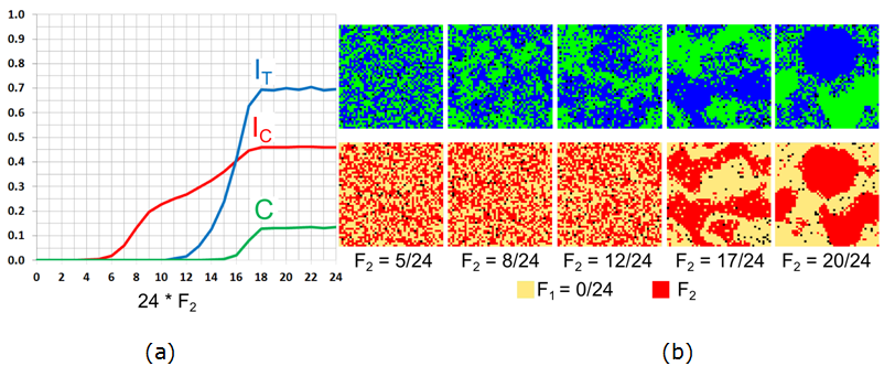
Figure 8. The case of \(F_1 = 0/24\) and varying \(F_2\): (a) Moran's I for agents' color (\(I_{\rm C}\)), tolerance (\(I_{\rm T}\)), and the \(C\)-index. (b) Color and tolerance patterns at \(t = 50{,}000\).

7.14

According to Figure 8, mixed patterns appear for the values of \(F_2\) for which the tolerance pattern is segregated. In this case, blue and green patches consist of intolerant \(F_2\)-agents, while integrated areas consist of completely tolerant \(F_1\)-agents.

7.15

It is important to note the importance of the value of \(F_2 = 0.5\) in the emergence of a mixed pattern. Indeed, for \(F_2 \leq 12/24\), the \(F_2\) agents who reside within the integrated patch of their own color can still be located at the boundary of the patch (Figure 8b, middle column). The pattern of tolerance remains thus integrated. However, for \(F_2 > 12/24\), \(F_2\)-agents cannot stay at the boundary of the color patch and must relocate into the inner part of the patch. Thus the boundaries of the color patches are occupied by the \(F_1\)-agents, and the pattern is segregated not only by color, but also by tolerance.

\(F_1 = 3/24\), \(F_2\) varies

7.16

When the \(F_1\)-agents react, even weakly, to their neighbors the dependence of the persistent pattern on \(F_2\) is different from the case of \(F_1 = 0\) (Figure 9). For \(F_2 \leq 6/24\) (and not 5/24, as above), the color pattern is integrated. Starting from \(F_2 = 7/24\), the level of color segregation (\(I_{\rm C}\)) gradually increases with the increase in \(F_2\) until reaching a maximum of 0.7 at \(F_2 = 12/24\). For this \(F_2\), the steady pattern consists of two segregated patches and only the boundary between the patches is integrated (Figure 9b, middle column).

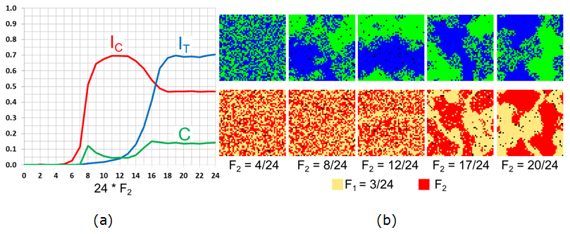
Figure 9. The case of \(F_1 = 3/24\) for varying \(F_2\): (a) Moran's I for agents' color (\(I_{\rm C}\)), tolerance (\(I_{\rm T}\)), and the \(C\)-index. (b) The patterns of agents' color and tolerance at \(t = 50{,}000\).

7.17

The level of tolerance segregation \(I_{\rm T}\) is non-zero for \(F_2 \geq 9/24\), since \(F_1\) agents concentrate at the boundaries of the green and blue patches (as in Figure 9b, middle column of \(F_2 = 12/24\)). Starting from \(F_2 = 13/24\), the value of \(I_{\rm C}\) decreases while the value of \(I_{\rm T}\) continues to increase, indicating that the segregated pattern is replaced by a mixed one. All three indices stabilize at \(F_2 = 16/24\), and the value of \(C \sim 0.15\) indicates that the patterns are mixed (Figure 9b).

7.18

Note that within the interval \(8/24 \leq F_2 \leq 15/24\), the model patterns are mixed, albeit the area of integration is smaller and the value of \(C\) varies between 0.05 and 0.1. The level of segregation by tolerance for these values of \(F_2\) is very low. We will show in Section 7.2.5 that this non-monotonous dependency is characteristic of \(F_1 = 3/24\).

\(F_1 = 5/24\), \(F_2\) varies

7.19

For the value of \(F_1 = 5/24\), which is near the tipping point value, an abrupt transition from integration to segregation is observed, as expected, when the tolerance threshold of the second half of the population passes it, i.e., at \(F_2 = 5/24\) (Figure 10). Then, segregation by tolerance starts at \(F_2 = 13/24\), when tolerant agents concentrate at the boundaries between the segregated patches (Figure 10b), but the patterns remain segregated until \(F_2 =17/24\). At \(F_2 = 18/24\), the integrated patch appears, the level of color segregation (\(I_{\rm C}\)) abruptly decreases, while the level of tolerance segregation grows rapidly. For all \(F_2 \geq 19/24\), the patterns are mixed and the indices stabilize.

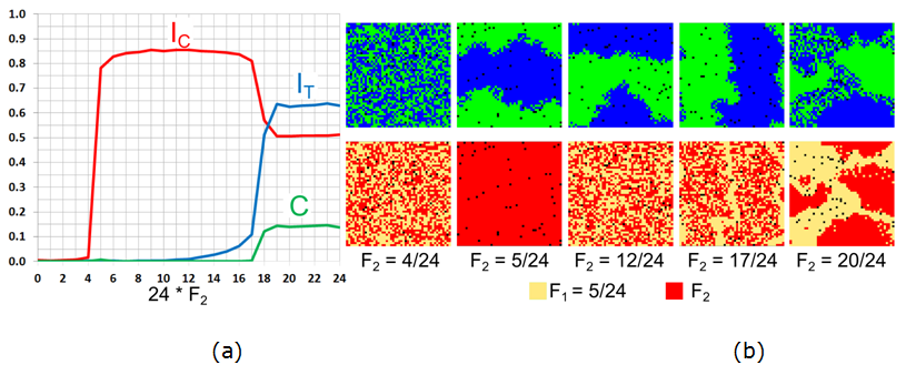
Figure 10. The case of \(F_1 = 5/24\) for varying \(F_2\): (a) Moran's I for agents' color (\(I_{\rm C}\)), tolerance (\(I_{\rm T}\)), and the \(C\) index. (b) The patterns of agents' color and tolerance at \(t = 50{,}000\).

\(F_1 = 7/24\), \(F_2\) varies

7.20

For \(F_1 = 7/24\), which is above the tipping point, the model exhibits a simple integration – segregation dichotomy and mixed patterns do not emerge (Figure 11). Segregation is reached abruptly at \(F_2 = 3/24\) and segregation by tolerance begins at \(F_2 = 13/24\), with the \(F_1\)-agents located along the border of the blue and green patches.

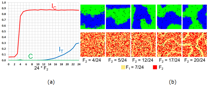
Figure 11. The case of \(F_1 =7/24\) and varying \(F_2\): (a) Moran's \(I\) for agents' color (\(I_{\rm C}\)), tolerance (\(I_{\rm T}\)), and the \(C\)-index. (b) The patterns of agents' color and tolerance at \(t = 50{,}000\).

Varying \(F_1\) and \(F_2\)

7.21

Figure 12 presents the values of the \(I_{\rm C}\), \(I_{\rm T}\) and \(C\) indices as dependent on \(F_1\) and \(F_2\) for \(\alpha = 0.5\) and \(\beta = 0.5\). The heat map of \(C\) (Figure 12c) confirms that a mixed pattern emerges when the tolerance of one of the subgroups is 5/24 or below, while the tolerance of the other subgroup is 16/24 or above. Tolerance patterns are also segregated in this case (Figure 12b).

7.22

It is convenient to consider the pattern change according to the \(F_1\)-values. For \(F_1 \in \{0/24, 1/24, 2/24\}\), segregation by color (\(I_{\rm C}\)) increases gradually with the increase of \(F_2\) until a mixed pattern is formed at \(F_2 = 13/24\), as indicated by the non-zero segregation by tolerance \(I_{\rm T}\). For these values of \(F_1\), segregation by tolerance exceeds segregation by color at \(F_2 = 17/24\). For \(F_1 \in \{3/24, 4/24, 5/24\}\), with the increase in \(F_2\), the pattern become segregated at the values of \(F_2\) close to the tipping point of \(F_2 = 5/24\) (Figure 12a), while a mixed pattern emerges, as above, for \(F_2 \geq 17/24\). In a few specific cases, the mixed pattern is not segregated by tolerance. These are cases of \(F_1 = 3/24\), \(F_2 \in \{8/24, \ldots, 14/24\}\) and of \(F_1 = 4/24\), \(F_2 = 6/24\) (Figure 12c).

7.23

Mixed patterns do not emerge for \(F_1 > 5/24\).

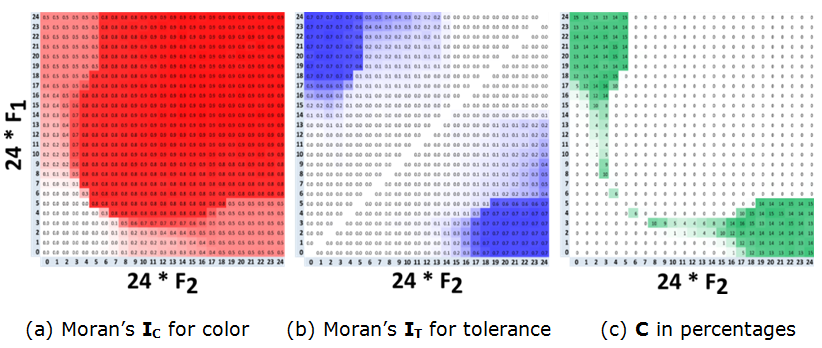
Figure 12. Heat maps for the three indices for arbitrarily \(F_1\) and \(F_2\), at \(t = 50{,}000\).

The dynamics of the mixed patterns

7.24

Let us use the example of \(F_1 = 3/24\) and \(F_2 = 20/24\) to demonstrate the development of the mixed patterns. This time, besides initial random patter, we also consider the initial pattern that is fully segregated by color and random according to the tolerance. Let us start with this pattern (Figure 13):

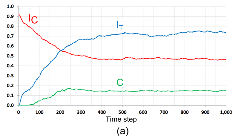
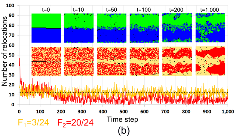
Figure 13. The development of a mixed pattern in the case of \(F_1 = 3/24\), \(F_2 = 20/24\). The initial pattern is segregated by color and random by tolerance. (a) The dynamics of \(I_{\rm C}\), \(I_{\rm T}\) and \(C\); (b) The dynamics of the number of relocations, by tolerance groups, and residential patterns at different time steps. The dashed line represents the expected number of relocations of satisfied agents (12.25 agents per time step).

7.25

According to Figure 13a, the level of color segregation (\(I_{\rm C}\)) of the model pattern decreases in time, while the level of segregation by tolerance (\(I_{\rm T}\)) and the level of mixing (\(C\)) increase. Visually, the boundary between the segregated parts of the pattern dissolves during first 100 iterations and then, towards time step 500, the tolerant \(F_1\)-agents form a steady integrated area (Figure 13b).

7.26

During the entire run, the number of migrating \(F_1\) agents who are highly tolerant, remains close to the expected number of random relocations (12 agents per iteration^[6], marked as a dashed horizontal line in Figure 13b). The relocation rate of intolerant \(F_2\)-agents is higher than the one of the \(F_1\)-agents at the first 200 time steps when \(F_2\)-agents near the boundary of the segregated patches relocate into the internal parts of the patches. As a result, the number of empty cells within the segregated patches decreases, while the number of empty cells within the integrated boundary area increases (see patterns for \(t > 200\)). As a result, cells that are suitable for the \(F_2\)-agents become rare, and the actual number of relocations of the \(F_2\)-agents, starting from \(t = 200\), decreases far below 12 (Figure 13b).

7.27

Figure 14 represents the model dynamics for the same values of \(F_1 = 3/24\), \(F_2 = 20/24\), for the initial pattern, where all \(F_1\)-agents are satisfied, while the \(F_2\) agents are not. As a result, more than 60% of the \(F_2\) agents relocate during the first time step. During next 50 time steps, the pattern segregates by color and the index of color segregation (\(I_{\rm C}\)) grows. The number of relocations of \(F_1\)-agents remains very close to 12. As in the case of the initially segregated pattern, \(F_2\)-agents avoid the boundaries of segregated patches and relocate to their internal parts. This initiates segregation by tolerance as reflected by the increasing measures \(I_{\rm T}\) and \(C\). Regardless of whether the initial pattern is segregated or random, for \(t = 200\) and further, the patterns' statistical characteristics are very close, while they remain visually different for a much longer period.

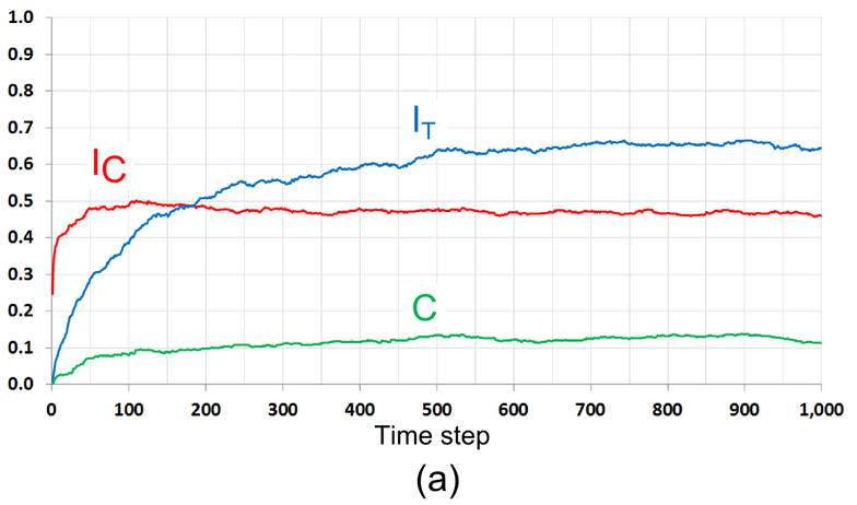
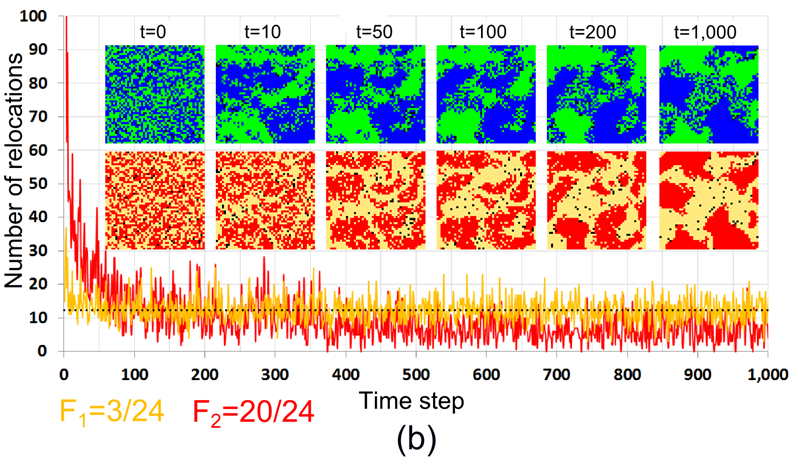
Figure 14. The development of a mixed pattern in the case of \(F_1 = 3/24\), \(F_2 = 20/24\). The initial pattern is integrated by color and by tolerance thresholds. (a) The dynamics of \(I_{\rm C}\), \(I_{\rm T}\) and \(C\); (b) The dynamics of the number of relocations by tolerance groups, and residential patterns at different time steps. The dashed line represents the expected number of relocations of satisfied agents (12.25 agents per time step).

Sensitivity of the steady pattern to the model parameters

7.28

In all our simulations, the number of \(F_1\) and \(F_2\) agents was equal (\(\alpha = 0.5\)), the number of blue and green agents was equal too (\(\beta = 0.\)5), the relocation rate of satisfied agents was low (\(m = 0.01\)), and the neighborhood was 5-by-5 cells. In this section, we explore the sensitivity of the major model result – the emergence of the mixed patterns to these parameters.

Sensitivity to the fraction \(\alpha\) of \(F_1\) agents

7.29

To investigate sensitivity to \(\alpha\) we consider the case of \(F_1 = 3/24\), \(F_2 = 20/24\) that is carefully studied above in the case of \(\alpha = 0.5\), and produces mixed patterns. The results of the study are presented in Figure 15.

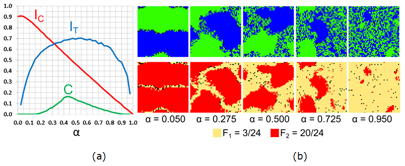
Figure 15. Varying the fraction \(\alpha\) of \(F_1\) agents for \(F_1 = 3/24\), \(F_2 = 20/24\): (a) Moran's I for agents' color (\(I_{\rm C}\)), tolerance (\(I_{\rm T}\)), and the \(C\)-index. (b) The patterns of agents' color and tolerance at \(t = 50{,}000\).

7.30

According to Figure 15, the size of the integrated patch is almost proportional to the value of \(\alpha\). When \(\alpha\) is close to zero, the pattern is segregated because highly intolerant \(F_2\) agents comprise the vast majority of the population. Few \(F_1\) agents are located at the boundary separating the blue and green patches (Figure 15b, \(\alpha = 0.05\)). With an increase in \(\alpha\), the size of the homogenous patches decreases, while the integrated area grows, as reflected in the steady decrease in the level of color segregation (\(I_{\rm C}\)). The level of segregation by tolerance (\(I_{\rm T}\)) and the level of mixing (\(C\)) grow, with the increase of \(\alpha\) up to \(\alpha = 0.5\). At \(\alpha = 0.5\), the size of the three regions is similar and the values of the \(I_{\rm T}\) and \(C\) are the highest. With the further increase of \(\alpha\), homogenous patches shrink and the integrated area dominates.

Sensitivity to the fraction \(\beta\) of blue agents

7.31

To study sensitivity to the fraction \(\beta\) of blue agents, we exploit the same case of \(F_1 = 3/24\), \(F_2 = 20/24\), keeping the fraction of \(F_1\) and \(F_2\) agents equal (\(\alpha = 0.5\)). The results of the study are presented in Figure 16.

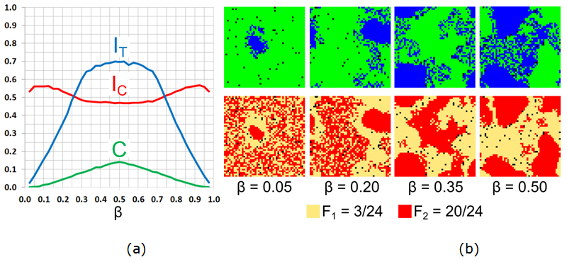
Figure 16. Varying the fraction \(\beta\) of blue agents for \(F_1 = 3/24\), \(F_2 = 20/24\): (a) Moran's I for agents' color (\(I_{\rm C}\)), tolerance (\(I_{\rm T}\)), and the \(C\)-index. (b) The patterns of agents' color and tolerance at \(t = 50{,}000\).

7.32

When the vast majority of agents are green (Figure 16b, \(\beta = 0.05\)), few blue agents form a small patch. Blue \(F_2\) agents reside within this patch. Blue \(F_1\) agents occupy the patch edge, but are too few to create a distinct integrated area. As \(\beta\) increases, the integrated area becomes apparent and grows until reaching a maximum at \(\beta = 0.5\). The level of segregation by color (\(I_{\rm T}\)) and the level of mixed integration and segregation (\(C\)) increase with the growth of \(\beta\) to 0.5 and then decrease, while \(I_{\rm C}\) behaves in the opposite manner.

Sensitivity to probability \(m\) of relocation of satisfied agents

7.33

To investigate the dependence of the mixed patterns on the probability \(m\) of relocation of a satisfied agent, we consider the case of \(F_1 = 3/34\) and vary the values of \(F_2\) and \(m\).

7.34

According to the heat maps (Figure 17), for \(F_2 \geq 18/24\), mixed patterns emerge for any \(m \geq 0.01\). For these values of \(F_2\), the tolerance pattern is always segregated (Figure 17b) and the value of \(C\) is high (Figure 17c).

7.35

The heat maps also indicate that, roughly, for a \(F_2\) between 8/24 and 17/24, the model produces a mixed pattern without the segregation of agents by tolerance. These mixed patterns are sensitive to the value of \(m\) and tend to diminish as \(m\) grows.

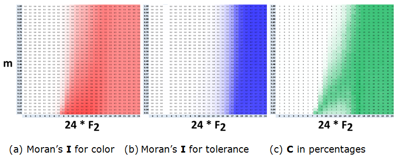
Figure 17. The dependence of the three indices on \(m\) and \(F_2\) for the case of \(F_1 = 3/24\) and \(\alpha\), \(\beta = 0.5\).

Sensitivity to the neighborhood's size

7.36

To test sensitivity of mixed patterns to the size of the neighborhood, we consider the case of \(F_1 = 0/24\), \(F_2 = 20/24\) and vary the neighborhood size from \(3\times3\) to \(9\times9\). In order to keep the neighborhood small relative to the grid size, we use a twice as large grid of \(100\times100\) cells. We also increase the number of empty cells \(w\) considered by agents when relocating from 30 to 120.

7.37

For the \(3\times3\) neighborhoods, the intolerant \(F_2\) agents produce many small homogeneous patches while the tolerant \(F_1\) agents occupy the boundaries of these patches and, in addition, produce integrated patches of a small size (Figure 18). For larger neighborhood sizes, the agents produce distinct mixed patterns that consist of two large homogeneous patches and an integrated area.

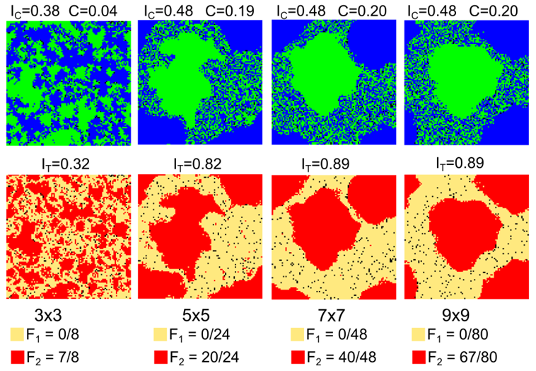
Figure 18. Steady mixed patterns for different neighborhood sizes. All indices are calculated based on \(5\times5\) neighborhoods.

7.4. Beta-binomial distribution of tolerance

7.38

To go beyond dichotomous distributions of tolerance, we consider cases where agents of both colors are assigned one of the 25 tolerance thresholds \(\{0/24, 1/24, \ldots, 24/24\}\) according to the Beta binomial family of distributions. To generate different Beta binomial distributions, we modifying the two shape parameters \(s_1\) and \(s_2\) of the Beta-binomial distribution: \(\mathbf{BB}(24, s_1, s_2)\). The numbers of blue and green agents are equal (\(\beta = 0.5\)).

Five qualitatively different Beta binomial distributions

7.39

We begin by comparing five qualitatively different Beta binomial distributions (Figure 19). The first is positively skewed and unimodal wherein the tolerance of about 1/3 of the agents is below the tipping point (\(F < 5/24\)) and the average is about 7/24 (Figure 19a). This distribution leads to a pattern that is mixed by color and integrated by tolerance (\(C = 0.07\), \(I_{\rm C} = 0.49\), \(I_{\rm T} = 0.02\)). The second case is symmetric and unimodal (Figure 19b) where only about 4% of the agents have a tolerance threshold below the tipping point and the average is 12/24, which is much higher than the tipping point. As expected, the steady color pattern is segregated, while the tolerance pattern remains integrated, \(I_{\rm C} = 0.84\), \(I_{\rm T} = 0.03\), \(C = 0\).

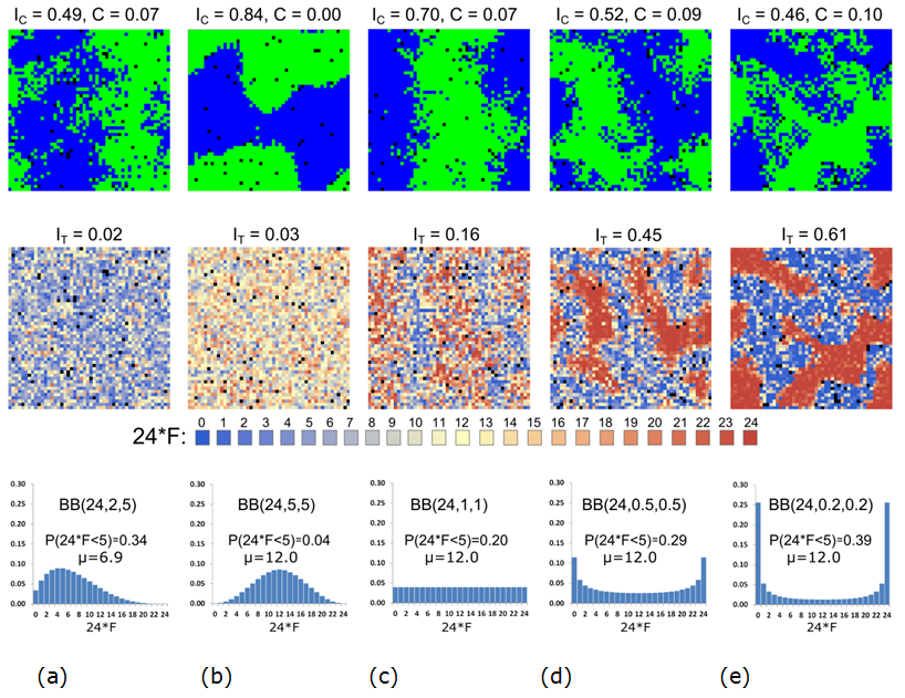
Figure 19. Steady color (top) and tolerance (middle) patterns for five distributions of tolerance thresholds (bottom), at \(t = 50{,}000\).

7.40

The third case is a uniform Beta binomial distribution (Figure 19c) with 20% of the agents having tolerance thresholds below the tipping point and an average of 12/24. The steady pattern in this case is segregated by color (\(I_{\rm C} = 0.70\)), with small integrated patches within the larger segregated areas (\(C = 0.07\)). The tolerance pattern is somewhat segregated (\(I_{\rm T} = 0.16\)) with a clear concentration of the tolerant agents on the boundary between the color patches. The fourth case is a symmetric U-shaped distribution with about 29% of the agents having tolerance thresholds below the tipping point (Figure 19d), and an average of 12/24 (Figure 19e). The color pattern is somewhat mixed (\(I_{\rm C} = 0.52\), \(C = 0.09\)), while the segregation of tolerance is high (\(I_{\rm T} = 0.45\)), still below \(I_{\rm C}\).

7.41

The fifth case (Figure 19e) is another symmetric U-shaped distribution with an even higher variance than in case four. The average tolerance in this case is 12/24 and 39% of the agents have tolerance thresholds below the tipping point. This distribution leads to a mixed color pattern that looks more distinct (\(C = 0.10\)) and a level of segregation by tolerance (\(I_{\rm T} = 0.61\)) that is higher than the level segregation by color (\(I_{\rm C} = 0.46\)).

Systematic study of Beta binomial distributions

7.42

The heat maps in Figure 20 depict the dependence of the model patterns on a larger set of 900 Beta binomial distributions that are defined according to the shape parameters \(s_1\) and \(s_2\). The characteristics of the outputs for symmetric distributions, where \(s_1 = s_2\), are located on the diagonal, the distributions that are skewed toward lower tolerances are above the diagonal and those skewed toward higher tolerances are situated below the diagonal (Figure 20, bottom right).

7.43

The heat map of the \(C\) index confirms that the most distinct mixed patterns are produced by U shaped distributions obtained for the values of \(s_1\), and \(s_2\) that are essentially lower than one. These distributions are characterized by the high fractions of agents with low and high tolerance thresholds. The \(I_{\rm T}\) heat map indicates that agents' tolerance is highly segregated in these patterns. The mixed patterns are preserved, but are less distinct (\(C < 0.1\)) as the U shaped distribution becomes unimodal (\(s_1, s_2 > 1\)).

7.44

In addition, the heat maps show that less distinct mixed patterns occur at the boundary between integrated and segregated patterns. More specifically, we can see that for \(s_1 \geq 1\) positive \(C\) values roughly follow the line \(s_2 = 3 \ast s_1- 1.4\). For these values of \(s_1\) and \(s_2\), the tolerance distribution is negatively skewed and the fraction of tolerant agents (\(F < 5/24\)) is about 30%. As shown in Section 7.4.1 (Figure 19a) in this case the mixed patterns occur even when the tolerance pattern is integrated.

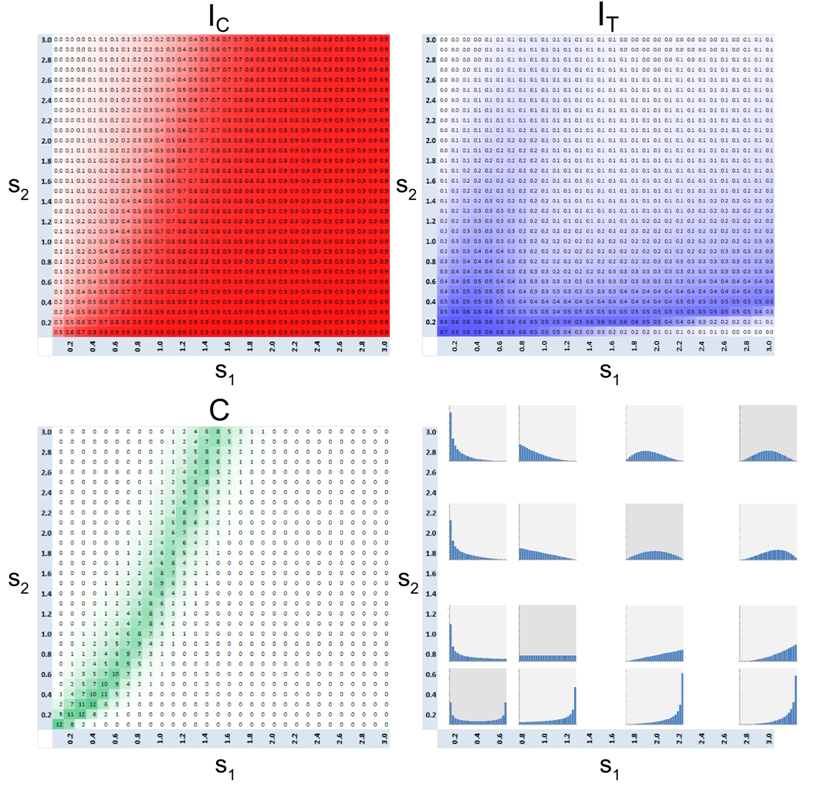
Figure 20. Dependence of \(I_{\rm C}\), \(I_{\rm T}\) and \(C\) on the parameters \(s_1\) and \(s_2\) of Beta-binomial distributions of agents' tolerance \(\mathbf{BB}(24, s_1, s_2)\). \(C\) index is shown in percentages.

Conclusions

8.1

The objective of our study was to investigate the conditions under which the Schelling model produces patterns that mix integration and segregation. Our interest in these patterns is not purely theoretical, but dictated by the ethnic patterns in many cities that are composed of homogeneous and heterogeneous neighborhoods. As we demonstrate, mixed residential patterns emerge when we relax the unrealistic assumption of a common tolerance and assume that different agents can have differing tolerance thresholds.

8.2

In dichotomous cases, when the agents' tolerance is either \(F_1\) or \(F_2\), the mixed patterns emerge in the model when the tolerance of the \(F_1\) agents is below ~21% (\(F_1 \leq 5/24\)), while agents of the second group need more than 2/3 of their neighbors to be friends (\(F_2 > 16/24\)). For these tolerance thresholds the \(F_1\)-agents are satisfied almost everywhere, while the \(F_2\)-agents are highly intolerant and seek neighborhoods with sufficiently high fractions of friends. The steady pattern of agents' tolerance in these cases is segregated and the blue and green \(F_2\)-agents form two segregated patches, while the \(F_1\) agents of both colors concentrate within the integrated areas that separate the patches of the \(F_2\)-agents.

8.3

For very low tolerance threshold of half of the agents, \(F_1 \leq 1/24\), varying the tolerance \(F_2\) of the other half from 0/24 to 24/24 causes a gradual transformation of the pattern from integrated to a mixed state. However, for \(F_1 \in [3/24, 5/24]\), the growth of \(F_2\) causes the pattern to first evolve from integration to segregation and only then from segregation to mixed.

8.4

Mixed patterns emerge because intolerant agents leave integrated areas and create dense blue and green patches with few empty cells inside. Integrated areas serve as wide extended boundaries between the segregated patches. Visually, tolerant agents reside within the integrated areas and, mostly, migrate within them for random reasons, while intolerant agents migrate within the segregated patches only. This happens because the residential opportunities available for the tolerant agents include both integrated areas and segregated patches of their color and, thus, are essentially wider that those for the intolerant ones.

8.5

As long as part of the population is tolerant, while the rest is highly intolerant, mixed patterns emerge regardless of other model parameters. In particular, the patterns remain mixed irrespective of the fraction \(\alpha\) of the \(F_1\)-agents, fraction \(\beta\) of blue agents, the rate \(m\) of random relocation, and the neighborhood size. Model parameters influence the size of the segregated and integrated patches, but not the mixed nature of the patterns that is always preserved.

8.6

If agents' tolerance thresholds are distributed over the entire \([0, 1]\) range, the mixed patterns became more distinct with the growth of the fraction of agents with extreme tolerance thresholds. In particular, U-shaped distributions produce distinct mixed patterns. Less distinct mixed patterns emerge when the tolerance of about one-third of the agents is below 5/24.

8.7

To conclude, the Schelling model produces mixed patterns due to the relocation of intolerant agents out of the integrated areas. Residential movements of this kind, such as the relocation of white residents out of ethnically integrated neighborhoods (Crowder 2000), might have indeed contributed to the formation of mixed patterns in cities. Additional factors, such as economic status and dwelling prices (Benard & Willer 2007; Fossett 2006; Hatna & Benenson 2011), are likely to provide deeper insight into the formation of mixed patterns as segregated and integrated neighborhoods may attract different economic segments of the residents' population of the same ethnicity.

8.8

While abstract models would allow identifying additional explanations for the formation of mixed patterns, residential models of real cities (Benenson et al. 2002; Yin 2009) could be exploited to assess their validity. Such spatially explicit models require a significant amount of data on the ethnic and socio-economic patterns of residence. Fortunately, these large quantities of data are being collected in many countries as part of recent national census programs, and small unit geographies (such as US census blocks and UK census output areas) offer a detailed view of the changing ethnic patterns.

Acknowledgements

Erez Hatna acknowledges support from J. M. Epstein's NIH Director's Pioneer Award, number DP1OD003874 from the National Institute of Health.

Notes

¹The Shannon entropy index also includes the census category "Other", which is not shown in Figure 2.

²In one of the variations of the linear model, where agent movement is restricted by distance, Schelling (1971, p. 153–154) formulated a similar mechanism where agents would move to a neighborhood with 3/8 friends, if no nearby neighborhood with the desired 4/8 exists.

³This number is determined using a computer program that builds all possible permutations of occupied/uncoupled cells for the \(n\times n\) neighborhood.

⁴For the specific parameters used in this study (density of \(d = 0.98\) and neighborhoods dimensions of \(5\times5\)), the highest value of \(I_{\rm C}\) is about 0.93.

⁵Note that all our estimates are based on finite 50,000-step simulations, and the pattern that remains integrated after 50,000 time steps may still segregate later. That is, the actual value of a tipping point as dependent on \(m\) may be slightly lower.

⁶The expected number of relocations, per iteration, of satisfied agents given that all their attempts are successful, is the product of \(m\) and the number of agents of each type: \(\beta \ast N \ast N \ast \mathrm{density} \ast m = 0.5 \ast 50 \ast 50 \ast 0.98 \ast 0.01 = 12.25\).

References

ANSELIN, L. (1995). Local indicators of spatial association–LISA. Geographical Analysis, 27(2), 93–115. [doi:10.1111/j.1538-4632.1995.tb00338.x]

ARNDT, C. (2004). Information measures: Information and its description in science and engineering. Signals and Communication Technology. Berlin: Springer.

BENARD, S., & Willer, R. (2007). A wealth and status-based model of residential segregation. Mathematical Sociology, 31(2), 149–174. [doi:10.1080/00222500601188486]

BENENSON, I., & Hatna, E. (2011). Minority-majority relations in the Schelling model of residential dynamics. Geographical Analysis, 43, 287–305. [doi:10.1111/j.1538-4632.2011.00820.x]

BENENSON, I., Omer, I., & Hatna, E. (2012). Entity-based modeling of urban residential dynamics - the case of Yaffo, Tel-Aviv. Environment and Planning B, 29, 491-512. [doi:10.1068/b1287]

BRUCH, E., & Mare, R. (2006). Neighborhood choice and neighborhood change. American Journal of Sociology, 112(3), 667–709. [doi:10.1086/507856]

BRUCH, E., & Mare, R. (2009). Preference and pathways to segregation: Reply to Van de Rijt, Siegel, and Macy, American Journal of Sociology, 114(4), 1181–1198. [doi:10.1086/597599]

CORNFORTH, D., Green D.G., & Newth, D. (2005). Ordered asynchronous processes in multi-agent systems. Physica D, 204, 70–82. [doi:10.1016/j.physd.2005.04.005]

CROWDER, K. (2000). The racial context of white mobility: An individual-level assessment of the White Flight Hypothesis. Social Science Research, 29, 223–257. [doi:10.1006/ssre.1999.0668]

ELLIS, M., Holloway, S.R., Wright, R., & Fowler, C.S. (2012). Agents of change: Mixed-race households and the dynamics of neighborhood segregation in the United States, Annals of the Association of American Geographers, 102(3), 549–570. [doi:10.1080/00045608.2011.627057]

FOSSETT, M.A. (2006). Including preference and social distance dynamics in multi-factor theories of segregation. Mathematical Sociology, 30(3–4), 289–298. [doi:10.1080/00222500500544151]

GLAESER, E., & Vigdor, J. (2012). The end of the segregated century: Racial separation in America's neighborhoods, 1890–2010. Manhattan Institute, Civic Report No. 66.

HATNA, E., & Benenson, I. (2011). Geosimulation of the income-based urban residential patterns. In D. Marceau and I. Benenson (Eds.), Advanced Geosimulation Models. Hilversum: Bentham Science Publishers.

HATNA E., & Benenson I. (2012). The Schelling Model of ethnic residential dynamics: Beyond the integrated–segregated dichotomy of patterns. Journal of Artificial Societies and Social Simulation, 15(1), 6 https://www.jasss.org/15/1/6.html

LOGAN J., & Stults B. (2011). The persistence of segregation in the metropolis: New findings from the 2010 census. Census Brief prepared for Project US2010. Retrieved from http://www.s4.brown.edu/us2010. Accessed June 19, 2014.

SCHELLING, T.C. (1969). Models of segregation. American Economic Review, 59, 488–493.

SCHELLING, T. C. (1971). Dynamic models of segregation. Mathematical Sociology, 1, 143–186. [doi:10.1080/0022250X.1971.9989794]

SCHELLING, T.C. (1974). On the ecology of micromotives. In The Corporate Society. Marris, R. (ed). (pp. 19–64) London: Macmillan.

SCHELLING, T.C. (1978). Micromotives and macrobehavior. New York: WW Norton.

VINKOVIC, D., & Kirman, A. (2006). A physical analogue of the Schelling model. Proceedings of the National Academy of Sciences, 103(51), 19261–19265. [doi:10.1073/pnas.0609371103]

XIE, Y., & Zhou, X. (2012). Modeling individual heterogeneity in racial residential segregation. Proceedings of the National Academy of Sciences, 109(29), 11646–11651. [doi:10.1073/pnas.1202218109]

YIN, L. (2009). The dynamics of residential segregation in Buffalo: An agent-based simulation. Urban Studies, 46(13). 2748–2770. [doi:10.1177/0042098009346326]