
Introduction
An inherent advantage of agent-based modeling is the possibility to model each agent individually, which makes it a promising method to investigate market dynamics. Simulating the modeled individuals permits emerging behavior to be explored (Kelly et al. 2013). Crucial to developing an agent-based model (ABM) is creating agents that are valid representations of their real-world counterparts. Until a few years ago, not many models in the ABM literature had a strong empirical foundation (cf. Janssen & Ostrom 2006;Wunder et al. 2013). Even when there was empirical foundation, the empirical data was often collected and integrated ad hoc, i.e., without reference to a defined methodology. However, in recent years great efforts have been made to increase the empirical foundation of ABMs, including step-wise descriptions of methods guiding from semi-structured stakeholder-interviews to implemented ABMs (Elsawah et al. 2015).
To further improve this situation, we present an approach where we have applied discrete choice experiments (DCEs) to elicit preferences of actors that are later represented as agents in our model. The term DCE is used according to the nomenclature for stated preference methods proposed by Carson and Louviere (2011). We demonstrate the potential of this approach with a case study of the Swiss wood market. The DCE was conducted with roundwood suppliers to quantify the decision model of the supplying agents. We present two approaches, latent class analysis and hierarchical Bayes, to evaluate the DCE data and show advantages and disadvantages of each approach to parameterize the model. The decision model is based on random utility theory and therefore contains a deterministic component, namely utility obtained through the DCE, and a random component accounting for non-measurable factors of an individual’s decision. We present a method to estimate the probability distribution of this random component and analyze its influence on the simulation results.
The Swiss wood market is a suitable market to explore the approach because importance of personal relationships between traders is above average for trading within the market (Kostadinov et al. 2014). DCEs are particularly useful for identifying the personal preferences that form and affect such relationships. If the approach proves to be suitable, we will extend our model to simulate scenarios that have been defined together with policy-makers and other stakeholders. It will then be applied to explore the effect of changes such as the market entrance of bulk consumers or subsidies that are introduced to increase wood availability. The project is embedded in a national research program which aims to increase availability of wood and expand its use (SNF 2010).
Related work
In the literature, many ABMs are described that use some kind of discrete choice model in the agents’ decision process. The data for the choice models stem from a wide range of sources, in some cases from estimations. However, only a few researchers used DCEs to improve the empirical foundation of their model.
Dia (2002) conducted a DCE with road users to study how they make route choice decisions in traffic jam situations. With his DCE, he looked for socio-economic variables that have significant influence on route choice decisions. After eliminating the non-significant variables, significant variables were applied to characterize agents giving them a corresponding utility function to evaluate route choice options.
Garcia et al. (2007) used a choice-based conjoint analysis (CBC) to calibrate an ABM of the diffusion of an innovation in the New Zealand wine industry. They recruited wine consumers to evaluate their decision making behavior and used the results from the CBC to instantiate, calibrate, and verify their ABM.
Hunt et al. (2007) linked ABMs and DCEs to study outdoor recreation behaviors. They compared the concepts of agent-based modeling and choice models and combined them in a case study. They used choice modeling to derive behavior rules, and used the simulated world of an ABM to illustrate and communicate the results.
Zhang et al. (2011) investigated the diffusion of alternative-fuel vehicles using an ABM approach. They conducted a CBC in conjunction with hierarchical Bayes to elicit the preferences of the consumer agents in the model. They used two utility functions in their model, where one is obtained by the CBC and the other by separate questions in the survey. While the utility function obtained by the separate questions includes an error term, the utility function obtained by CBC does not, which would be required in random utility theory.
Gao and Hailu (2012) used an empirically based random utility model to represent the behavior of angler agents in a recreational fishing model. The behavioral data is based on multiple surveys from different sources. Angler agents choose angling sites based on individual characteristics and attributes of the alternative sites.
Arentze et al. (2013) implemented a social network as an ABM where the probability of a person being a friend with another person depends on a personal utility function. The utility function accounts for social homophily, geographic distance, and presence of common friends. It is based on the random utility model and therefore includes an error term. The authors use a revealed preference method to gather the model data by asking survey participants about characteristics of their existing friendships.
Lee et al. (2014) used an ABM to simulate energy reduction scenarios of owner-occupied dwellings in the UK. The agents in the model were home-owners which had to decide, triggered by certain events, if they want to carry out any energy efficiency improvement in their house. The decision-making algorithm originates in DCE data from two separate studies, where the population was divided into seven clusters with similar preferences. The preferences of the agents in each cluster were distributed around the center point of the cluster to provide a heterogeneous population. The utility function of the agents are deterministic, i.e. without error component.
It is striking that where combinations of ABMs and DCEs are applied in the literature, the role of the error component and how it is modeled are often neglected or at least not explicitly mentioned. However, the error component is central to random utility theory, which is the theoretical foundation of DCEs. This paper contributes to this field by rigorously adhering to random utility theory that underlies the DCE method to improve the empirical foundation of ABMs.
Description of the Model
This section describes the model according to the ODD + D protocol (Müller et al. 2013), which extends the ODD protocol (Grimm et al. 2006 and 2010) to be more suitable for describing the decision-making process of the agents. The focus of this paper is more on the method than on the model; however, as especially the design of the DCE is not separable from its application area, a rough understanding of the model is needed before the method can be described in detail. This is another reason why the following description aims at giving sufficient information to understand the model, not to enable exact replication.
Overview
Purpose
The model represents the wood market in Switzerland and is used to simulate scenarios such as the market entrance of bulk consumers or a fluctuating exchange rate. The goal of these simulations is to identify factors influencing the wood availability on the market. The model is used by the authors, while the simulation results are reported to the appropriate stakeholders.
Entities, state variables, and scales
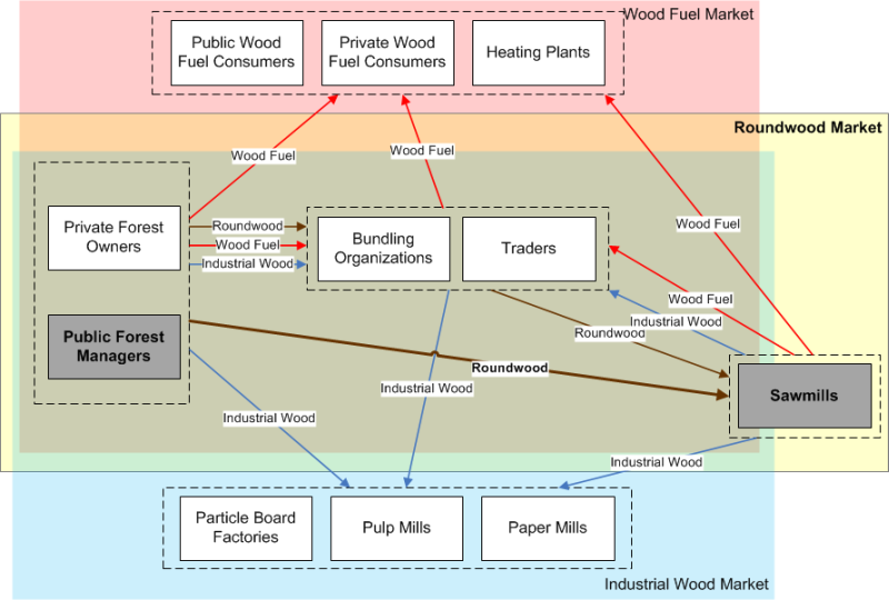
Entities: Entities in the model are different types of agents which act within one or more markets (Figure 1). However, to reduce complexity for the reader, we present our approach eliminating all but two agent types from the market. This is possible because the main assortment on the Swiss wood market is roundwood, and there is only one type of consumer on the market for it: sawmills. Two supply agent types exist in the roundwood market, namely private forest owners and public forest managers. Since the majority of roundwood is harvested and sold by public forest managers (hereafter referred to as foresters), the private forest owners are also omitted in this paper. The wood fuel market and the industrial wood market are dependent on the roundwood market, because wood fuel and industrial wood are by-products that accumulate during the roundwood harvesting and production process. These two by-products can be omitted in this paper because they do not have a direct impact on the main product roundwood.
State variables:
- Each agent has a location (x-/y-coordinate) and a portfolio of goods he buys or sells.
- Every agent has a confidence value for each and every contractual partner between which negotiations have taken place. The confidence increases after successful negotiations leading to a contract and decreases if negotiations fail.
- Foresters have a certain monthly harvesting capacity, sawmills have a monthly processing capacity.
Scales: One time step represents one month, simulations were run for 20 years.
Process overview and scheduling
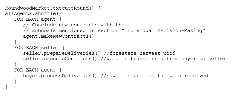
A forest year starts in September and ends in August of the following year. Each month proceeds in three steps: in the first step, all agents are shuffled and then one after the other negotiates new contracts with other agents. In the second step, foresters prepare their deliveries, i.e. they harvest wood and deliver to their contractual partners. In the third step, sawmills process the wood received from the foresters. This process is also described as pseudocode in the appendix.
Design Concepts
Theoretical and Empirical Background
The conceptual model of agents and interactions was created and continuously refined based on semi-structured interviews and workshops with different wood market actors and stakeholders.
The decision model of the agents is based on random utility theory, which is the basis of several models and theories of decision-making in psychology and economics (Adamowicz 1998). Random utility theory is based on the work of McFadden (1974), who extended the concepts of pairwise comparisons introduced by Thurstone (1927). According to random utility theory, a person choosing between multiple alternatives chooses the one with the highest utility, where the utility function is defined as U = V + ε, with U being the total unobservable utility, V the deterministic observable component of the consumer’s behavior, and ε a random component representing the non-measurable factors of an individual’s decision. This error term has a probability distribution that is specific to the product and the consumer. In our model, such a utility function is used by each agent to negotiate new contracts. Agents evaluate incoming and outgoing potential transactions by considering five decision criteria. This leads to the following form of the utility function:
| $$U = V + \epsilon = \beta_1c_1 + \beta_2c_2 + \beta_3c_3 + \beta_4c_4 + \beta_5c_5 + \epsilon$$ | (1) |
| $$\Delta U = U - \beta_None$$ | (2) |
The part-worth utilities of the decision criteria can be assigned to each agent individually, per group of agents, or they can be equal for all agents. Our approach to obtain the part-worth utilities will be explained in the method section.
Individual Decision-Making
Agents of different types pursue different objectives:
- Forester agents try to harvest a certain amount of wood during each forest year. The target amount of wood is determined by the annual allowable cut. However, the target amount per month differs greatly between the seasons because of various restrictions such as snowfall in winter and increased risk of logging damages in summer. This is implemented in the model by assigning each forester agent with a minimum, optimal, and maximal monthly harvesting amount that takes seasonal variability into account. The minimum and maximum amounts are attributed to the manpower available to each forester; employees must be kept busy, but also have a maximum working capacity. Therefore, to reach the targeted yearly amount, the foresters harvest an amount of wood each month close to the optimum, while balancing monthly variations. To achieve their objective they continuously plan the coming months in the current forest year and negotiate suitable contracts.
- Sawmill agents always try to maintain sufficient wood stocks for continuous processing. They negotiate new contracts based on their demand, which is almost constant throughout the year, with only minor reductions during periods when less wood can be harvested. They have warehouses to balance the reduced wood availability during certain periods and include the warehouse capacity utilization in their planning processes.
When agents negotiate with potential contractual partners, they have to evaluate the potential transaction to see if it is acceptable or not. For this purpose, each agent considers several decision criteria, which are defined for each agent type.
Forester agents consider the following five decision criteria to evaluate a potential transaction. The criteria were identified in semi-structured interviews and workshops with foresters and other domain experts:
- Amount of wood available. Foresters generally try to harvest approximately the amount of wood each year that regrows in a year, but never more. Employees have to be kept busy. Therefore, there is pressure to sell enough wood during the year.
- Amount of wood demanded. Larger order sizes reduce transaction costs, but also increase concentration risks.
- Trust in demander. On the Swiss wood market, wood is usually traded without written contracts. Furthermore, the exact price paid for the logs is determined based on the measurements at the sawmill.
- Margin. The net amount of money a forester receives (= price + subsidies – harvesting costs – transportation costs).
- Expected price development. Foresters have some tolerance in the annually harvested amount of wood, i.e., they can adapt the amount based on the expected price development. For example, if they expect rising prices, they can postpone the sale of wood to a later date.
Sawmill agents consider five different decision criteria to evaluate potential transactions. However, they are conceptually similar to those of the foresters:
- Urgency. The sawmills must have a constant degree of capacity utilization. Supply bottlenecks can usually be absorbed by the warehouse stock, but stock may not be sufficient especially in the seasons when only little wood is harvested. This can place a high urgency on obtaining additional supplies.
- Size of order. Larger order sizes reduce transaction costs.
- Trust in supplier. Supplies have to be on time and complete.
- Price. Higher prices reduce the margin of the sawmill.
- Expected price development. If prices are expected to drop and the warehouse stock is not empty, a sawmill can wait for lower prices until making new purchases.
Learning
Learning is not included in the model.
Individual Sensing
- Agents know the average market prices of previous months and use this information in their decision process.
- If an agent contacts another agent between whom no previous negotiation has taken place, there exists no confidence value for this agent. In such cases the confidence value is calculated by averaging the confidence other agents have with the respective contractual partner. This, in effect, can be considered the reputation of the contractual partner.
Individual Prediction
The expected price development in the coming months is calculated using the information about past months’ market prices, and is a criterion in agents’ decision process.
Interaction
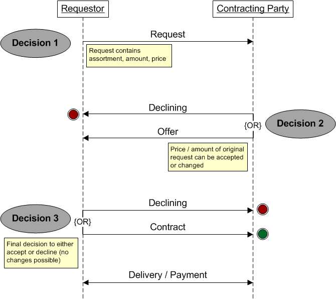
Figure 2 depicts how agents interact with one another, i.e. how they negotiate a new contract. The interaction is initiated by the requestor, who can be either a buyer or a seller. He sends a request including the assortment, the amount, and the price to a potential contracting party. The contracting party can then either decline the request or respond with an offer. The price and the amount in the offer can be different than in the request. Finally, the requestor has the opportunity to either accept or decline the offer. There are no further rounds of negotiation in a single interaction, as bargaining is unusual on the roundwood market in Switzerland. Therefore, this interaction pattern induces three situations where a decision has to be made. These decisions are made according to the approach presented in Design concepts (see 3.7).
Collectives
Each agent has a personal address book with potential contractual partners in his nearby area. Aside this, there are no collectives in the model.
Heterogeneity
All forester agents have a forest with equal size and have equal harvesting capacity. All sawmill agents have the same processing capacity. Their aggregate capacity corresponds to the amount of wood that forester agents are able to harvest; respectively supply and demand are balanced. In the reduced model presented here, import and export within the modeled region are ignored. The two agent types differ in the criteria they consider in their decisions. The considered criteria are always the same per agent type, but the weighting of the criteria may differ from agent to agent.
Stochasticity
- The location of all agents is randomly determined during initialization.
- Agents negotiate new contracts in a random order in each simulated month.
- At the beginning of the simulation, agents select potential contractual partners randomly, later they prefer to negotiate with agents they already know from previous contracts.
- As long as agents do not have a contract history, prices are randomly set (Gaussian distribution).
- The utility value calculated in the decision process contains a random component reflected in the error term ε (see ).
Observation
Several approaches were used to test, analyze, evaluate, and finally validate the model:
- Evaluation of aggregated results. A multitude of variables are calculated over all agents for each simulated month. These variables include average, minimum, and maximum values for prices, traded amounts, monetary situation of agents, etc. The values are stored in a CSV file and are then predominantly evaluated graphically.
- Evaluation of individual variables for each agent. Some variables are examined in more detail, i.e., not just minimum/average/maximum values over all agents are recorded, but the specific value for each agent. This is done for variables such as degree of capacity utilization in the warehouse or of production, and also allows the recognition of interesting patterns in the simulation results. This approach uses CSV files as well and was also applied to track a fitness variable which will be presented in the method section.
- Individual agent evaluation. This approach traces some randomly selected agents in detail over the whole simulation period. Almost all important data about an agent is stored in an XML file for each simulated point in time, and thus permits further evaluation with a separate evaluation program. For example, this data enables an understanding of the reasons why each and every incoming or outgoing request was accepted or rejected. This approach is especially valuable if bugs are to be traced back to their source.
- Visual evaluation. It is possible to run the simulation program with a GUI that includes a map containing all agents. Arrows depict interactions of buyers and sellers live during the simulation. This approach permits a monitoring of agents in their geographical contexts, which would otherwise be difficult using the methods mentioned above.
Details
Implementation Details
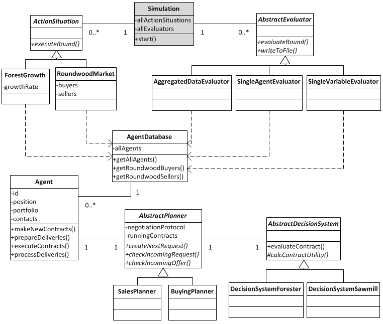
The model was implemented in Java, a simplified UML class diagram is depicted in the appendix. The model was tested and validated on the one hand with the approaches mentioned in the above section, which are based on face validity (Sargent 2005) and mainly require the interpretation of graphs. On the other hand, Java assertions were used in many methods to enable continuous testing during the development process. They make it possible to insert preconditions, postconditions, and invariants within the code, making the code easier to read and maintain.
Initialization
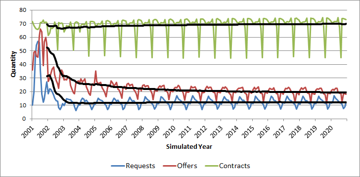
A random seed can be set to initialize the simulation permitting the results to be reproducible (cf. Stochasticity), which is an important prerequisite for the validation of a model (Amblard et al. 2007). At the beginning of a simulation run, agents have to conclude contracts with other agents without an available contractual history. Therefore, initially the contract properties such as the contracting party and the price are selected randomly. With a growing contract history from several simulation rounds, agents will attempt to build contracts that are similar to previous successful contracts. It follows that after an initial phase business relationships become relatively stable (Figure 3). This substantiates the observation that over time most business relationships tend towards stability on the Swiss wood market.
Method
Discrete Choice Experiments
To know how individuals make decisions, their preferences need to be elicited. In our case, this implies that the attributes of a potential transaction considered in a decision situation must be known (cf. sections on Individual Decision-Making and Interaction). These attributes and their importance can be identified by means of preference elicitation methods, of which a multitude exist. We concluded that DCEs are most suitable for our case, since they are based on random utility theory (RUT), like the decision model of the agents in our model (cf. section Theoretical and Empirical Background). DCEs are stated preference methods; while these have a slightly lower accuracy than revealed preference methods, they have the advantage that an arbitrary number of choice situations can be presented to an individual.
A central point in RUT is the error term. Using the standard choice-based conjoint analysis (CBC) approach that is not based on RUT, evaluating utility functions results in choice probabilities for different alternatives. However, these choice probabilities are purely based on mathematical theories and not on theories of human behavior or their preferences as in RUT (Louviere 2010). CBC and DCEs both lead to coefficients (also known as “betas”) that describe the part-worths of individual attributes for a given target group.
As described in the section Theoretical and Empirical Background, the error term ε of a utility function has a probability distribution that is specific to the product and the individual consumer. This is represented in the model by drawing the error term from a normal distribution that was initialized with a random seed. This seed is based on a combination of (i) the agent’s ID, (ii) the ID of the current negotiation with the contract partner, and (iii) the random seed that was used to initialize the simulation. This procedure guarantees that if the same offer has to be evaluated multiple times by an agent, the error term is always the same.
Experimental Setup
In our DCE, only the selling side of the roundwood market was considered. We conducted the experiments with foresters in two Swiss cantons, Canton of Aargau (AG) and Canton of Grisons (GR). We chose these two regions since they show some fundamental differences. First, AG is flat, while GR is mountainous. The mountainous terrain in GR increases harvesting costs, which reduces the profitability of harvesting. There is also a lot of protection forest where harvesting is prohibited entirely. Second, although AG and GR are both border cantons, GR is much more affected by the wood market of the adjacent countries. For this paper we decided to demonstrate our approach only on AG, as this enables us to eliminate the aforementioned peculiarities of GR, which are interesting for the overall study, but would introduce too much noise in the results for the specific purpose of this paper.
Carson and Louviere (2011) categorized the different types of DCEs. Three related approaches are: choice questions (one chooses the preferred option), ranking exercises (all options are ranked), and best-worst choice questions (the best and the worst option are chosen). Foster and Mourato (2002) showed that ranking exercises with larger choice-sets (ranking many options) can lead to inconsistencies in the results. Caparrós et al. (2008) showed that choice questions lead to similar results as ranking exercises that include only the first rank in the evaluation. Akaichi et al. (2013) confirmed this for small choice-sets with only three options.
To avoid the problems of ranking larger choice-sets, we used best-worst choice questions where each question has three options. Best-worst choice questions with three options are similar to ranking experiments. Having exactly three options leads to a complete ordering of the options and thereby increases the number of implied binary comparisons (Carson & Louviere 2011). Additionally, even though that in a best-worst DCE a respondent is asked for more information than in a DCE where only the preferred option has to be chosen, the cognitive effort is not much higher, as the respondent already evaluated all alternatives in the set to choose the best (Lancsar et al. 2013).
One of the three options presented in our experiment is a “status quo alternative”. Having a status quo alternative has the advantage of always offering a feasible choice to the respondent (Carson & Louviere 2011).

Figure 4 shows an example of a decision situation used in our experiment. In each decision situation, the subject had to select the best and the worst options out of three. Two of them were options to sell wood, and one was a “don’t sell” option, which was to be chosen if the subject would rather wait for other offers before selling wood. The two selling options each had five attributes, corresponding to the decision criteria explained in the section Individual Decision-Making, and each attribute could take on three different levels (Table 1). All attributes were quantitative, which later facilitates the integration of the DCE results into the ABM. Twelve decision situations were presented to each subject. The influence of such design dimensions – number of attributes, number of levels, number of decision situations – on DCE results have been studied by Caussade et al. (2005). They found that particularly a large number of attributes, but also a large number of levels, have a negative influence on the respondents ability to choose. We considered this point by reducing the attributes and levels to an acceptable minimum. A subsequent study by Rose et al. (2009) showed that the influence of the design dimensions also differs between countries, in particular for the number of decision situations to assess. When Bech et al. (2011) investigated the influence of the number of decision situations on DCE results, they found that even presenting 17 decision situations to each respondent does not lead to problems. However, their results also indicated that the cognitive burden may increase with more decision situations presented. Since we had a relatively low number of potential respondents, we needed to ask as many decision situations per subject as possible, while being careful to not fatigue or even completely discourage the subjects from responding. Therefore we decided that for our study presenting 12 decision situations to each respondent is a reasonable compromise between these two subgoals.
The experimental design (combinations of attribute-levels presented to the subjects) is a controlled random design where all subjects are given different versions of the questionnaire. In this case controlled random design means that the levels are balanced, i.e. each level is presented approximately an equal number of times. Level overlap is allowed to occur, i.e. in a single decision situation an attribute can have the same level in both options presented.
| Attribute | Levels | Explanation |
|---|---|---|
| Amount of wood available | 70% / 40% / 15% | Amount of wood that has not yet been sold compared to the yearly total amount that can be sold |
| Amount of wood demanded | 15% / 10% / 1% | Size of order compared to the yearly total amount that can be sold |
| Trust in demander | 0.2 / 0.5 / 0.8 | 1 = highest trust, 0 = no trust |
| Margin | CHF 25 / CHF 10 / CHF -5 | Net margin per m3 in Swiss Francs |
| Expected price development | +10% / 0% / -10% | Expected price in a year in relation to current price |
DCE Evaluation and Agent Parameterization
There are several methods for evaluating DCEs. We used the following three, because each of them is useful for a specific purpose that we consider valuable for ABMs:
- Logit. This evaluation method measures the average preferences of the population by regarding all actors as having equal preferences. This method provides a good starting point to evaluate DCEs, as it gives an overview of the whole population. However, since logit assumes that all agents have equal preferences, much of agent individuality, which is one of the major strengths of ABMs, is lost. The method is described in more detail by Sawtooth Software (2015) and Hosmer and Lemeshow (1989).
- Latent Class Analysis (LCA). This method divides the sample into several classes of subjects with similar preferences. Using LCA in combination with choice-based conjoint analysis was first proposed by DeSarbo et al. (1995).
- Hierarchical Bayes (HB). The individual preferences of each subject in the sample are estimated. This method became popular at the end of the nineties, as it requires much more computational effort as the other two methods mentioned above. Early uses of this method are described by Allenby and Lenk (1994), Allenby and Ginter (1995), and Lenk et al. (1996).
The DCE was designed and evaluated using the Sawtooth 8.3 software. A comparison of this software with other DCE design approaches can be found in Johnson et al. (2013). The evaluation of the DCE leads to a part-worth utility value for each attribute level and one for the “don’t sell”-option, the none-option. Therefore three values for the part-worth utilities are obtained per attribute, one for each level. A linear regression leads to the coefficients of V, the deterministic observable part of the utility function (cf. Equation 1). While the betas are obtained from the DCE, the error term \(\epsilon\) is randomly generated during simulation. It has a mean of zero and a variable standard deviation. An approach to calculate the standard deviation is presented in the next section.
For privacy reasons, the forester agents have random locations that do not conform to the real locations of the corresponding DCE subjects. We assume that this is acceptable, since we do not see any considerable regional distinctions in our study region where this procedure might introduce errors. Additionally, we repeated our simulations multiple times mapping the DCE data differently each time, which should further reduce potential errors.
Estimating the Standard Deviation of the Error Term
In order to evaluate if a request can be accepted or not, one has to compare its utility against the utility of the none-option (Equation 2). This is achieved by calculating the observable deterministic part of utility (V) of the request with the part-worth utilities obtained by evaluating the DCE (Figure 5, step 1). If this value V plus the error term is greater than the utility of the none-option (\(\beta_None\)), the request is accepted, as random utility theory states that always the option with the highest utility is chosen.
The evaluation of the DCE is based on the Multinomial Logit model (MNL), which states that when these two utility values are exponentiated, the ratio of the resulting values corresponds to the probability that the request can be accepted (Figure 5, step 2).
Our model should comply with random utility theory, therefore the utility functions must have the form of \(U = V + \epsilon\). The option with the highest utility is selected and thus a request is accepted if:
| $$V + \epsilon \geq \beta_None \text {or} \epsilon \leq V - \beta_None$$ | (3) |
Therefore it is possible to select the standard deviation of \(\epsilon\) in such a way that the resulting probability distribution leads to an equal choice probability as the one obtained in the MNL model (Figure 5, step 3).

However, the distribution of \(\epsilon\) calculated in this way only accounts for the uncertainty in the MNL model. According to random utility theory, the error term \(\epsilon\) also accounts for unobserved product attributes or characteristics of the deciding individual (Manski 1977). Therefore it might be possible that the standard deviation σ of the error term needs to be higher than calculated above. This can be solved by increasing the standard deviation for each agent individually with a factor that is based on the accuracy of the subject’s answers. However, since the error term is not measurable, we cannot know its exact probability distribution. The general influence of the magnitude of σ on the model is discussed in the results section.
Enhancing ABMs with DCEs
Our goal is to enhance ABMs with DCEs by improving the empirical foundation of the model and benefitting from the well-established random utility theory. Empirical information can be used either as input data or to test a model (Janssen & Ostrom 2006). Our approach uses the DCE data as input data for the decision model of each forester agent.
As (empirical) validity is not measurable, but rather a subjective human judgment (Amblard et al. 2007), it is difficult to quantify to what extent the ABM is enhanced by the empirical data and thus to assess the success of our approach. Additionally, the extent to which the ABM is enhanced would depend on the accuracy of the estimated decision behavior without having empirical data from the DCE. Hilty et al. (2014) describe this as the problem of defining the baseline. We therefore assess our approach by performing a parameter variability-sensitivity analysis (Sargent 2005). With this validation method, we check the plausibility of the simulation output when agents are parameterized with the results from the DCE. We focus on control variables of which their evolution in reality and under normal market conditions is known. By using the validation methods described in the section Observation, we ensure that these observed variables always stay within a realistic range over the entire simulation period. This is, the behavior of the market participants in our simulation is compared with the expected behavior in reality. To illustrate this process, we identified one variable as a fitness measure. This variable is explained in the following section.
The reasons explained above prevent a real proof that our approach does in fact enhance ABMs; however, we are convinced that including empirical data in a model is in most cases an improvement of a model. By including empirical data on the micro level we also aim at a higher structural validity (cf. Zeigler 2000) of the model, as we try to generate the macro behavior with a similar mechanism as in the real system. It may be possible that a model with "invented" (non-empirical) decision parameters would perform better regarding the model validity on the macro-level, but this would prevent from understanding the causal mechanisms inside the ABM. This is discussed in detail by Boero & Squazzoni (2005), where they state (2.13): "[..] what else, if not empirical data and knowledge about the micro level, is indispensable to understand which causal mechanism is behind the phenomenon of interest?".
Observed Fitness Variable
In our study region (cf. section Experimental Setup), foresters try to equate yearly wood sales to the level of yearly wood growth, as long as no storm damages occur. This means that the amount of wood sold annually per forester can be assumed to be nearly constant, as it depends mainly on the size of the forest. We define our fitness variable as the ratio of roundwood sold in one year to the amount of wood that is regrown in the same period and usable as roundwood. Harvesting more wood in one year than the amount that regrows is not allowed, which is regulated by the determination of the annual allowable cut. Therefore the defined fitness variable should always have a value very close to one, but not greater.
Because we know which value this variable should normally have, it is ideally suited for checking the plausibility of the DCE results. In our DCE, the foresters had to imagine themselves being involved in the presented situation and decide how they would react in it. Therefore, the 12 decision situations presented to each subject only represent 12 arbitrary situations in a year. A problem of such stated preference methods is the possibility that a subject indicates decision behavior that does not conform to reality. In our case, this would mean that if we equip each forester agent with the indicated decision behavior obtained from the DCE, it could lead to too few or too many transactions in the model. This would imply that the decision behavior parameters are not plausible.
Simulation Procedure
The current version of the simulation program is intended to verify the suitability of using DCEs to parameterize an ABM and to evaluate different approaches to integrating the DCE data. Therefore only a standard market situation without any special market events (e.g., entry of new market participants) is simulated. In the simulated market situation, the margins of the foresters are rather low, but still within the range that was covered by the DCE. This procedure is necessary because if the margins were very high, the foresters would almost always sell, and there would be little to observe.
In each simulation run, a period of 20 years is simulated. The first three years of the simulation are ignored in the analysis to avoid bias due to the initialization phase (cf. Figure 3). Because the model is stochastic, each simulation run is repeated 100 times using different random seeds.
Results and Discussion
Comparison of Hierarchical Bayes and Latent Class Analysis
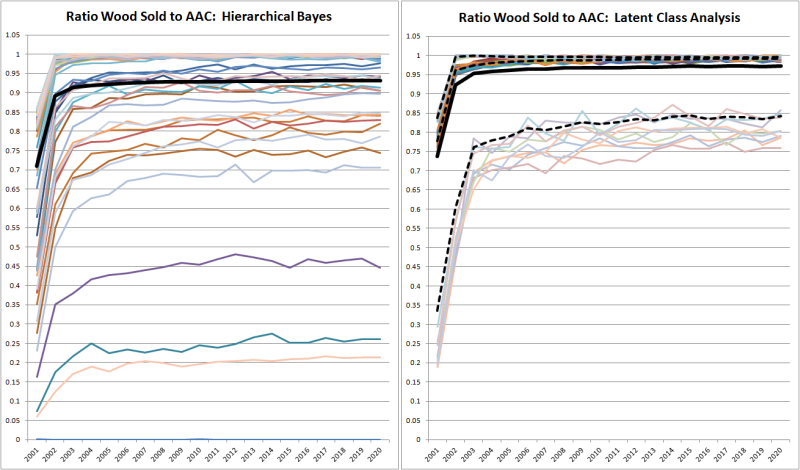
Latent class analysis (LCA) can divide a sample into an arbitrary number of classes; for simplicity’s sake, we used an example with three and later one with two classes. To illustrate the consequences of using either hierarchical Bayes (HB) or LCA to parameterize the decision behavior of the agents, a comparison of the two approaches is presented in Figure 6. In order to check the plausibility of the decision behavior parameters, we observe the fitness variable defined above, which should always have a value very close to one. The error term is set to zero in this example permitting a better comparison of the results.
Each approach has its specific advantages and disadvantages. Since HB estimates an individual utility function for each DCE respondent, it is very sensitive to the answers the respondents give. This also implies that respondents who do not respond with reasonable care (reasons may be, e.g., reluctance or fatigue) provoke utility functions and therefore decision behavior parameters that make it impossible to survive on the market. One such possible case occurs if a forester agent never sells, although he should. This can be observed in the left diagram of Figure 6; there are three forester agents who sell less than half of the available roundwood, and one who does not sell anything at all. This leads to an average of the observed variable of around 93%. It should be noted that the first three years of the simulation are omitted from the calculation of the averages (see Section on simulation procedures.
The right diagram in Figure 6 shows the simulation results when the agents are initialized with LCA parameters using three classes of agents. The overall average is slightly higher with 97%. However, if per-class averages are examined, a similar phenomenon can be observed. There are two classes with an observed value of about 99%, and one class with an average value of about 82%. The latter class contains nine of the 80 foresters modeled.
Whether HB or LCA is the more appropriate approach firstly depends on the quality of the DCE survey data and secondly on the scenarios to be simulated. Low data quality, for example caused by subjects reluctantly participating in the DCE, might lead to implausible results when using HB. This effect might be reduced by manually sorting out the data of some respondents. However, this poses a risk for a selection bias, and it might be difficult to differentiate between low data quality and unusual but existing decision behavior. LCA is more robust to such outliers, but also reduces the diversity of decision behaviors. Whereby it is this diversity in which each market participant can be modeled with an individual way of deciding that is one of the key benefits that agent-based simulations provide.
A Closer Look at Latent Class Analysis
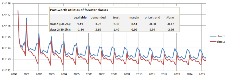
Figure 7 shows the per-class average price foresters receive for roundwood when they are divided into two classes using LCA. Two interesting phenomena can be observed. First, the class that gives more weight to the margin criterion (class 1) also achieves higher prices. Second, in class 1 the prices rise towards the end of the forest year, while in the class 2 they fall. This can be explained by looking at the coefficients for the criterion “amount of wood available”: class 1 has a positive coefficient, while class 2 has a negative one. A positive coefficient means that a forester is more likely to sell wood whilst still having a large amount of available wood, i.e., at the beginning of the forest year. Therefore, there is a tendency to negotiate higher prices towards the end of the year. The class with the negative coefficient behaves conversely. Note that the average simulated market price after several rounds is largely independent on the initial price level given at the start of the simulation. As we simulate a business-as-usual scenario without external influences such as import/export or scenarios of over- or undersupply, the price solely emerges from the utility functions of the agents.
With LCA, the subjects in the sample can be divided into an arbitrary number of classes. The model builder must choose the appropriate number of classes. When consulting experts operating in the Swiss wood market with the two- and three-class parameter set, they clearly favored the two-class approach. They could not imagine that there are foresters that rate all attributes more or less the same, as a class with about 10% of the subjects indicated in the three-class approach. The simulation which applied three classes confirmed their expectation that the behavior of the agents in this 10% class is rather implausible. Because such an effect can only be verified in a simulation, simulating results obtained by DCEs also increases the transparency of these results. However, an explanation for such behavior, while seemingly implausible, might be that product attributes that are important in the decision of an individual were not included in the DCE. This shows the importance of the error term of the utility function, which accounts for such cases.
Influence of the Error Term
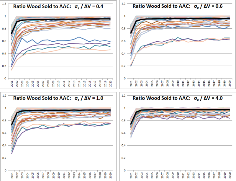
Figure 8 illustrates how the magnitude of the error term \(\epsilon\) influences the simulation results. The standard deviation of the error term is set in relation to the average ΔV (see Figure 5) and is varied between 40% and 400% of the average ΔV. The observed variable is again the fitness variable described above, the ratio between roundwood sold and the annual allowable cut, which should always be close to one. It can be observed that the variance of the curves decreases with an increasing standard deviation of the error term. The reason for this effect is in the error term whereby increasing its standard deviation respectively increases the randomization of the entire utility function. This means that utility functions which previously resulted in very low market activity now have a higher probability of allowing normal market participation. However, this leads to the effect that more negotiation rounds are necessary when the standard deviation increases. The additional negotiation rounds compensate for the increased randomness in the utility function; if the randomness is high, the probability that lucrative offers are rejected and unprofitable ones accepted increases. Therefore, a high standard deviation of the error term also leads to lower cost-effectiveness of the market. However, including the error term in the utility functions is important, as otherwise they are no longer consistent with random utility theory (cf. section Discrete Choice Experiments; Louviere 2010).
Challenges of the Approach
Several challenges emerge when using DCEs to parameterize an ABM. The first challenge is data collection. The number of attributes and levels in the DCE must be in accordance with the number of subjects in the survey, the sample size. A rule of thumb for DCEs with aggregated analysis is defined by Johnson and Orme (2003) and Orme (2009). They recommend calculating the minimum sample size with
| $$n \geq \frac{500 * c}{t * a}$$ | (4) |
A more general statement was made by Lancsar and Louviere (2008): “one rarely requires more than 20 respondents per version to estimate reliable models”. We were able to conduct almost a full population survey (n=55, N=ca. 80), though the absolute number of subjects was still not very high. The problem was also exacerbated in that some respondents felt the survey method overly theoretical, which may have reduced the data quality. However, we suppose that a population data coverage of 70% is sufficient for the given purpose.
Another problem is “how to derive observations of a social system over time” (Janssen and Ostrom 2006) or, in other words, “using cross-sectional data to estimate parameters of function forms of agents’ decisions” Villamor et al. (2012). This problem also occurs when conducting DCEs. Even when multiple hypothetical decision situations are presented to each subject; we might face the problem that the subject has the current market situation in mind, which might influence his decision. It is therefore possible that we would obtain different data if the real market situation changed. If it is not possible to repeat the experiment at different points in time, this problem could be reduced by considering in the DCE more attributes per option that also take the market situation into account. However, adding more attributes complicates data collection, because more respondents or more questions per respondent are necessary.
Finally, we only collected data from the selling side of the market, which directly influences the interaction with the forester agents. This is the case because forester agents might be faced with nonsensical requests or offers from sawmill agents that can for instance lead to an unrealistic shift of market power. This can only be avoided by estimating and calibrating the sawmills’ decision behavior parameters with reasonable care.
One way to address some of the problems mentioned could be to automatically adapt the utility function of each agent during simulation. This could be achieved through learning algorithms that adapt the utility functions in small steps to the changed simulated market conditions. However, this would weaken the empirical foundation on which the original DCE was created.
Conclusion and Outlook
We presented an approach combining DCEs with ABMs and conclude that DCEs are a suitable method to enhance the empirical foundation of ABMs. We demonstrated this approach within a case study of a Swiss roundwood market. By observing a fitness variable, we were able to state that the decision behavior parameters of the agents obtained through the DCE are plausible for most agents. For the small share of seemingly unusual decision behavior, the standard deviation of the error term can be increased, which is in accordance with random utility theory. We presented a method to calculate this standard deviation and demonstrated how increasing it leads to increased randomness of decisions and hence lower cost-effectiveness of the market.
The comparison of latent class analysis (LCA) and hierarchical Bayes (HB) as DCEs evaluation methods prove in both cases to be useful for evaluating DCEs and integrating the results into an ABM. While LCA is more robust to outliers (which may originate from low data quality), HB is better suited to the agent paradigm as each individual agent can have his own empirically based decision behavior.
As the approach of enhancing ABMs with DCEs looks promising for our application, our next step will be to conduct the DCE with the buying side of the wood market. Our goal is to implement a model of the Swiss wood market containing all three major wood assortments and corresponding agent types (cf. Figure 1). This will enable us to simulate scenarios that can provide decision support for policy-makers and other interested parties.
Acknowledgements
This work is part of the project "An economic analysis of Swiss wood markets", which is funded by the Swiss National Science Foundation through its National Research Program “Resource Wood” (NRP 66).Appendix
UML Class Diagram
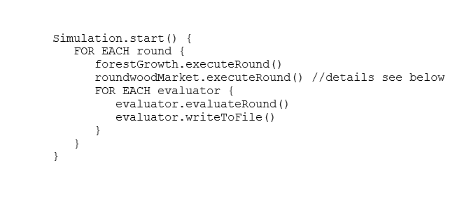
Pseudocode
DCE data
| Percentage | Available | Demanded | Trust | Margin | Price Trend | None |
| 0.521 | 1.10765 | 3.71545 | 2.29954 | 0.13907 | -0.50003 | -0.17317 |
| 0.365 | -1.33519 | 2.69343 | 1.39942 | 0.08656 | 2.93641 | -2.36081 |
| 0.114 | -2.76458 | 7.73036 | 2.43698 | 0.06526 | 15.15206 | -0.26193 |
| Respondent id | Available | Demanded | Trust | Margin | Price Trend | None |
| 1 | -1.65021 | 11.74185 | 1.48699 | 0.15045 | 27.9498 | -0.32893 |
| 2 | 0.00152 | 2.7108 | 5.86578 | 0.09515 | -4.68225 | -0.34429 |
| 3 | -0.93907 | 5.69982 | 5.73421 | 0.17154 | 9.39712 | -1.73636 |
| 4 | -0.20594 | 2.33914 | 6.60405 | 0.23196 | -10.79376 | 0.31855 |
| 5 | 0.48267 | 5.1465 | 1.14684 | 0.01039 | 4.58829 | -1.69116 |
| 6 | -0.05803 | 5.31644 | 3.92213 | 0.20255 | -2.34701 | 1.46233 |
| 7 | 3.53005 | 4.62726 | 0.43271 | 0.08359 | 9.86007 | -0.74989 |
| 8 | 1.03595 | 1.81 | 1.26642 | 0.01212 | -6.1483 | -4.34665 |
| 9 | 1.29175 | 3.2495 | 3.28484 | 0.22383 | 2.36744 | -3.70485 |
| 10 | -0.72595 | 5.86004 | 1.67825 | 0.26147 | 6.32396 | -4.58434 |
| 11 | -3.7714 | 12.07729 | 1.70283 | -0.03799 | 25.765 | -2.91517 |
| 12 | -0.64134 | 8.66919 | 0.58588 | 0.85216 | 15.23726 | -2.73378 |
| 13 | -2.38885 | 9.75864 | 2.67844 | 0.24657 | 19.48115 | -3.76842 |
| 14 | 1.47113 | 1.94409 | 5.63944 | 0.15977 | -8.73772 | 0.94164 |
| 15 | 0.44531 | 5.3594 | 3.3253 | 0.19398 | 0.54057 | -0.40329 |
| 16 | 0.68513 | 6.56316 | 0.70069 | 0.1629 | 4.2541 | 0.09896 |
| 17 | -0.69656 | 6.18657 | 4.20723 | 0.34206 | -0.80857 | 3.16604 |
| 18 | 1.11296 | 6.6634 | 3.31843 | 0.84481 | 8.06414 | -0.74866 |
| 19 | 0.43058 | 8.34134 | 1.61603 | 0.24749 | 10.11763 | -0.26094 |
| 20 | 0.52809 | 3.32461 | 3.3177 | 0.18038 | -8.54455 | -1.11341 |
| 21 | 1.03296 | 4.5115 | 4.35263 | 0.05935 | 6.28141 | -0.5846 |
| 22 | -2.57125 | 10.19657 | 0.41028 | 0.00238 | 9.9161 | -2.34199 |
| 23 | -1.96979 | 2.11568 | 2.3026 | 0.0533 | -20.95443 | -1.47928 |
| 24 | 2.65001 | 3.70051 | 1.57828 | 0.84137 | 8.09823 | -2.12457 |
| 25 | -0.01849 | 6.02466 | 2.32619 | 0.11939 | -1.67464 | -0.15444 |
| 26 | -0.71414 | 4.73313 | 4.6687 | 0.23562 | -5.16314 | -0.9748 |
| 27 | -0.90609 | 5.99437 | 4.26545 | 0.03039 | 7.9698 | 0.26158 |
| 28 | 2.24163 | 3.11603 | 2.7478 | 0.21428 | -1.59987 | -2.08913 |
| 29 | -0.80157 | 5.809 | 2.49672 | 0.30295 | 8.62159 | -3.36045 |
| 30 | -1.78717 | 8.37476 | 4.15142 | 0.11689 | 15.34745 | -1.11911 |
| 31 | 2.60449 | -0.18525 | 2.17123 | 0.13614 | -10.09713 | -0.3845 |
| 32 | -0.88535 | 5.57735 | 3.11717 | 0.10382 | 4.42179 | -2.89004 |
| 33 | 1.25579 | 5.57075 | 2.49091 | 0.16504 | 4.07795 | -0.52886 |
| 34 | 0.5901 | 3.62148 | 3.9655 | 0.79139 | -8.39507 | 1.37867 |
| 35 | -2.45724 | 9.34384 | 2.73292 | 0.29417 | 16.68159 | -3.43844 |
| 36 | 0.10763 | 5.43047 | 3.14805 | 0.23269 | -0.64867 | -1.32549 |
| 37 | -2.24524 | 10.24467 | 1.1318 | 0.09598 | 9.4068 | 0.99438 |
| 38 | -0.30457 | 9.82876 | -0.06199 | 0.056 | 20.60886 | -0.59821 |
| 39 | 0.9982 | 6.18441 | 0.79915 | 0.25892 | 10.17568 | -2.38179 |
| 40 | 0.58834 | 3.92607 | 3.35001 | 0.07797 | 2.16074 | -4.57116 |
| 41 | -1.66035 | 3.96522 | 3.93209 | -0.00443 | -1.15795 | -3.02296 |
| 42 | -1.97189 | 7.22988 | 1.38998 | 0.1213 | 11.93619 | -5.62056 |
| 43 | 0.82819 | 4.7467 | 0.9625 | 0.22142 | 3.96102 | -0.63942 |
| 44 | 1.54494 | 6.12931 | 3.13649 | 0.82428 | 8.72477 | -1.06492 |
| 45 | 1.95801 | 4.49723 | 2.90722 | 0.08472 | 7.18297 | 0.98367 |
| 46 | 1.04304 | 4.29444 | 1.97797 | 0.29028 | 5.68395 | -4.11341 |
| 47 | -2.3322 | 10.35659 | 2.32305 | 0.42228 | 18.24946 | -2.65153 |
| 48 | -0.97862 | 6.06758 | 4.7696 | 0.22328 | 0.21119 | -0.12754 |
| 49 | 0.6094 | 4.66721 | 0.57257 | 0.12686 | -6.20349 | -0.75471 |
| 50 | -2.8735 | 7.12722 | 3.65683 | 0.06123 | 7.4203 | -3.33714 |
| 51 | 0.51633 | 7.26817 | 2.54608 | 0.12281 | 7.2992 | -2.4483 |
| 52 | 0.54491 | 3.98197 | 3.23532 | 0.19742 | 2.13933 | -4.80881 |
| 53 | -2.37632 | 10.46205 | -1.59661 | 0.20672 | 15.16371 | -3.85899 |
| 54 | 2.29437 | 0.31326 | 4.51728 | 0.35852 | -15.97996 | 2.14107 |
| 55 | -0.66437 | 8.80765 | 2.02634 | 0.13916 | 22.59912 | -4.28693 |
References
ADAMOWICZ, W., Louviere, J. & Swait, J. (1998). Introduction to Attribute-Based Stated Choice Methods. Report. Submitted to National Oceanic and Atmospheric Administration, USA.
AKAICHI, F., Nayga, R. M. &Gil, J. M. (2013). Are Results from Non-hypothetical Choice-based Conjoint Analyses and Non-hypothetical Recoded-ranking Conjoint Analyses Similar?. American Journal of Agricultural Economics, 95(4), 949-963. [doi:10.1093/ajae/aat013]
ALLENBY , G. M., & Ginter, J. L. (1995). Using extremes to design products and segment markets. Journal of Marketing Research, 32, 392-403. [doi:10.2307/3152175]
ALLENBY , G. M., & Lenk, P. J. (1994). Modeling household purchase behavior with logistic normal regression. Journal of the American Statistical Association, 89(428), 1218-1231. [doi:10.1080/01621459.1994.10476863]
AMBLARD , F., Bommel, P., & Rouchier, J. (2007). Assessment and validation of multi-agent models. Multi-Agent Modelling and Simulation in the Social and Human Sciences, 93-114.
ARENTZE, T. A., Kowald, M. & Axhausen, K. W. (2013). An agent-based random-utility-maximization model to generate social networks with transitivity in geographic space. Social Networks, 35(3):451-459. [doi:10.1016/j.socnet.2013.05.002]
BECH, M., Kjaer, T., & Lauridsen, J. (2011). Does the number of choice sets matter? Results from a web survey applying a discrete choice experiment. Health economics, 20(3), 273-286. [doi:10.1002/hec.1587]
BOERO, R. & Squazzoni, F. (2005). Does empirical embeddedness matter? Methodological issues on agent-based models for analytical social science. Journal of Artificial Societies and Social Simulation, 8(4) 6: https://www.jasss.org/8/4/6.html.
CAPARRÓS, A., Oviedo, J. L. & Campos, P. (2008). Would you choose your preferred option? Comparing choice and recoded ranking experiments. American Journal of Agricultural Economics, 90(3), 843-855. [doi:10.1111/j.1467-8276.2008.01137.x]
CARSON, R.T. & Louviere, J.J. (2011). A Common Nomenclature for Stated Preference Elicitation Approaches. Environmental and Resource Economics.49:539-559. [doi:10.1007/s10640-010-9450-x]
CAUSSADE, S., de Dios Ortúzar, J., Rizzi, L. I., & Hensher, D. A. (2005). Assessing the influence of design dimensions on stated choice experiment estimates. Transportation research part B: Methodological, 39(7), 621-640. [doi:10.1016/j.trb.2004.07.006]
DESARBO, W. S., Ramaswamy, V., & Cohen, S. H. (1995). Market segmentation with choice-based conjoint analysis. Marketing Letters, 6(2), 137-147. [doi:10.1007/BF00994929]
DIA, H. (2002). An agent-based approach to modelling driver route choice behaviour under the influence of real-time information. Transportation Research Part C: Emerging Technologies. 10(5-6):331-349. [doi:10.1016/S0968-090X(02)00025-6]
ELSAWAH, S., Guillaume, J. H., Filatova, T., Rook, J. & Jakeman, A. J. (2015). A methodology for eliciting, representing, and analysing stakeholder knowledge for decision making on complex socio-ecological systems: From cognitive maps to agent-based models. Journal of Environmental Management, 151, 500-516. [doi:10.1016/j.jenvman.2014.11.028]
FOSTER, V. & Mourato, S. (2002). Testing for consistency in contingent ranking experiments. Journal of Environmental Economics and Management, 44(2), 309-328. [doi:10.1006/jeem.2001.1203]
GAO, L. & Hailu, A. (2012). Ranking management strategies with complex outcomes: an AHP-fuzzy evaluation of recreational fishing using an integrated agent-based model of a coral reef ecosystem. Environmental Modelling & Software, 31, 3-18. [doi:10.1016/j.envsoft.2011.12.002]
GARCIA, R., Rummel, P. & Hauser, J. (2007). Validating agent-based marketing models through conjoint analysis. Journal of Business Research, 60(8):848-857. [doi:10.1016/j.jbusres.2007.02.007]
GRIMM, V., Berger, U., Bastiansen, F., Eliassen, S., Ginot, V., Giske, J., Goss-Custard, J., Grand, T., Heinz, S.K., Huse, G., Huth, A., Jepsen, J.U., Jørgensen, C., Mooij, W.M., Müller, B., Pe’er, G., Piou, C., Railsback, S.F., Robbins, A.M., Robbins, M.M., Rossmanith, E., Rüger, N., Strand, E., Souissi, S., Stillman, R.A., Vabø, R., Visser, U. & DeAngelis, D.L. (2006). A standard protocol for describing individual-based and agent-based models. Ecological Modelling, 198(1-2):115-126. [doi:10.1016/j.ecolmodel.2006.04.023]
GRIMM, V., Berger, U., DeAngelis, D.L., Polhill, J.G., Giske, J. & Railsback, S.F. (2010). The ODD protocol: A review and first update. Ecological Modelling, 221(23):2760-2768. [doi:10.1016/j.ecolmodel.2010.08.019]
HILTY, L. M., Aebischer, B. & Rizzoli, A. E. (2014). Modeling and evaluating the sustainability of smart solutions. Environmental Modelling & Software, 56, 1-5. [doi:10.1016/j.envsoft.2014.04.001]
HOSMER, D. W., & Lemeshow, S. (1989). Applied Logistic Regression. John Wiley & Sons.
HUNT, L.M., Kushneriuk, R. & Lester, N. (2007). Linking agent-based and choice models to study outdoor recreation behaviours: a case of the Landscape Fisheries Model in northern Ontario, Canada. For. Snow Landsc. Res., 81,1/2:163-174.
JANSSEN, M.A. & Ostrom, E. (2006). Empirically based, agent-based models. Ecology and Society, 11(2):37.
JOHNSON, R. & Orme, B. (2003). Getting the Most from CBC.Sawtooth Software Research Paper Series.
JOHNSON, F. R., Lancsar, E., Marshall, D., Kilambi, V., Mühlbacher, A., Regier, D. A., Bresnahan, B. W., Kanninen, B., & Bridges, J. F. (2013). Constructing experimental designs for discrete-choice experiments: report of the ISPOR conjoint analysis experimental design good research practices task force. Value in Health, 16(1), 3-13. [doi:10.1016/j.jval.2012.08.2223]
KELLY, R. A., Jakeman, A. J., Barreteau, O., Borsuk, M. E., ElSawah, S., Hamilton, S. H., Henriksen, H. J., Kuikka, S., Maier, H. R., Rizzoli, A. E., van Delden, H. & Voinov, A. A. (2013). Selecting among five common modelling approaches for integrated environmental assessment and management. Environmental Modelling & Software, 47, 159-181. [doi:10.1016/j.envsoft.2013.05.005]
KOSTADINOV, F., Holm, S., Steubing, B., Thees, O. & Lemm, R. (2014). Simulation of a Swiss wood fuel and roundwood market: An explorative study in agent-based modeling. Forest Policy and Economics, 38: 105-118. [doi:10.1016/j.forpol.2013.08.001]
LANCSAR, E. & Louviere, J. (2008). Conducting discrete choice experiments to inform healthcare decision making. Pharmacoeconomics, 26(8), 661-677. [doi:10.2165/00019053-200826080-00004]
LANCSAR, E., Louviere, J., Donaldson, C., Currie, G., & Burgess, L. (2013). Best worst discrete choice experiments in health: Methods and an application. Social Science & Medicine, 76, 74-82. [doi:10.1016/j.socscimed.2012.10.007]
LEE, T., Yao, R., & Coker, P. (2014). An analysis of UK policies for domestic energy reduction using an agent based tool. Energy Policy, 66, 267-279. [doi:10.1016/j.enpol.2013.11.004]
LENK, P. J., DeSarbo, W. S., Green, P. E., & Young, M. R. (1996). Hierarchical Bayes conjoint analysis: Recovery of partworth heterogeneity from reduced experimental designs. Marketing Science, 15(2), 173-191. [doi:10.1287/mksc.15.2.173]
LOUVIERE, J.J., Flynn, T.N. & Carson, R.T. (2010). Discrete choice experiments are not conjoint analysis. Journal of Choice Modelling, 3(3):57-72. [doi:10.1016/S1755-5345(13)70014-9]
MANSKI, C.F. (1977). The structure of random utility models. Theory and Decision, 8(3): 229 - 254. [doi:10.1007/BF00133443]
MCFADDEN, D. (1974). Conditional Logit Analysis of Qualitative Choice Behavior. Frontiers in Econometrics, ed. by P. Zarambka. New York: Academic Press.
MÜLLER, B., Bohn, F., Dreßler, G., Groeneveld, J., Klassert, C., Martin, R., Schlüter, M., Schulze, J., Weise & H., Schwarz, N. (2013). Describing human decisions in agent-based models – ODD + D, an extension of the ODD protocol. Environmental Modelling & Software, 48, 37-48. [doi:10.1016/j.envsoft.2013.06.003]
ORME, B. (2009). Sample Size Issues for Conjoint Analysis. Retrieved July 14, 2015, from: http://www.sawtoothsoftware.com/support/technical-papers/general-conjoint-analysis/sample-size-issues-for-conjoint-analysis-studies-2009..
ROSE, J. M., Hensher, D. A., Caussade, S., de Dios Ortúzar, J., & Jou, R. C. (2009). Identifying differences in willingness to pay due to dimensionality in stated choice experiments: a cross country analysis. Journal of Transport Geography, 17(1), 21-29. [doi:10.1016/j.jtrangeo.2008.05.001]
SARGENT, R. G. (2005). Verification and validation of simulation models. Proceedings of the 37th Conference on Winter Simulation, 130-143. [doi:10.1109/wsc.2005.1574246]
SAWTOOTH SOFTWARE (2015). Estimating Utilities with Logit. Retrieved November 13, 2015, from: https://www.sawtoothsoftware.com/help/issues/ssiweb/online_help/estimating_utilities_with_logi.html..
SNF (Swiss National Foundation) (2010). Retrieved February 20, 2015, from the Website of National Research Programme NRP 66 Resource Wood: http://www.snf.ch/en/researchinFocus/nrp/nrp66-resource-wood/..
THURSTONE, L. L. (1927). A law of comparative judgment. Psychological review,34(4), 273. [doi:10.1037/h0070288]
VILLAMOR, G. B., van Noordwijk, M., Troitzsch, K. G. & Vlek, P. L. G. (2012). Human decision making in empirical agent-based models: pitfalls and caveats for land-use change policies. Proceedings 26th European Conference on Modelling and Simulation, 631-637. [doi:10.7148/2012-0631-0637]
WUNDER, M., Suri, S. & Watts, D. J. (2013). Empirical agent based models of cooperation in public goods games. Proceedings of the fourteenth ACM conference on electronic commerce, 891-908. [doi:10.1145/2492002.2482586]
ZHANG, T., Gensler, S. & Garcia, R. (2011). A study of the diffusion of alternative fuel vehicles: an agent-based modeling approach. Journal of Product Innovation Management, 28(2): 152-168. [doi:10.1111/j.1540-5885.2011.00789.x]
ZEIGLER, T., Praehofer, H., & Kim, T. G. (2000). Theory of modeling and simulation: integrating discrete event and continuous complex dynamic systems, Academic press.