
Introduction
The Brazilian tax system is paradoxical, with high taxes, dual tax systems (taxes and contributions) and fierce fiscal war between federated members (Afonso, Romero & Monsalve 2013). The complexity of the tax system becomes more obvious and striking when considering the subnational entities. The post-1988 constitutional decentralization imposes the same competences to very heterogeneous municipalities (Rezende 2010). Municipalities have different administrative, technical, and political capacities, besides their inherently differentiated borrowing leverage (Canuto & Liu 2013). This heterogeneity among municipalities occurs not only in relation to budgetary magnitude, but also in relation to the disparity between central and peripheral municipalities in metropolitan and regional context (Antinarelli 2012; Rezende & Garson 2006). Indeed, Furtado et al. (2013) identified that there are significantly fewer resources to metropolitan peripheral municipalities vis-à-vis the central city and non-metropolitan municipalities. The authors also suggest that such municipalities are administratively inefficient, with poorer results. In addition to this reduced administrative and financial capacity, peripheral municipalities still have worse quality of life and higher levels of violence (Andrade & Figueiredo 2005; Waiselfisz 2012). There is a huge amount of literature on public spending efficiency (Afonso et al. 2013; Gasparini & Miranda 2011; Orair et al. 2011), which contains actual policy propositions (Afonso 2014; Gobetti 2015), is descriptive (Santos & Gouvêa 2014), and of a high-quality level. However, few exercises emphasize the prospective analysis that simulates future effects of present public policy change (Brandalise, Rojo, da Mata, & de Souza 2012; Carvalho, Oliveira, & Oliveira 2015), especially for the case of Brazil and its subnational entities. Another trend of literature discusses federalism and optimal economic criteria to determine federal entities boundaries (Olson 1969; Oates 1972; 1999). However, these authors recognize that most limits are imposed by history rather than rational reasoning. Specifically for metropolitan regions, Bahl (2010) provides a theoretical panorama and details international financing experiences.
Computer simulation models for macroeconomic analysis and taxes (Dawid et al. 2012; Dosi et al. 2012; Dosi, Fagiolo & Roventini 2009), banking and finance (Cajueiro & Tabak 2005, (2008; Tabak, Cajueiro & Serra 2009), stock exchange (LeBaron 2006; Palmer et al. 1994) and energy market (LeBaron & Tesfatsion 2008), to name a few applications, abound. These studies were developed from the seminal works of Anderson, Pines and Arrow (1988) and Arthur (1994). Recently, advances in this literature includes models that discusses bank interconnections by means of network analysis and systemic fault possibilities (Bargigli & Tedeschi 2014; Grilli, Tedeschi, & Gallegati 2014; Ya-Qi et al. 2013).
This abundant literature, however, looks at specific markets (banking, energy or exchange markets) or seek to represent markets and its agents and processes in detail, so that they quickly become complex and demanding high computing power (Guocheng et al. 2015; Van Der Hoog, Deissenberg, & Dawid 2008).
Simple models that intend to model the interaction among actors in short-term spatial scales are rare. Tesfatsion (2006) makes an initial proposal of a model with two products (hash and beans) whereas Straatman et al. (2013) proposed a framework that simulates a market auction linked to a production model that together result in a simple model, but complete and micro founded.
Lengnick (2013) expands the work of Gaffeo et al. (2008) and proposes a model that simulates macroeconomic variables, contains elements of real estate and goods and labor markets. As detailed below, our proposal is based on Lengnick’s model, but makes several changes, including explicit spatial location in the housing market, and subnational administrative regions.
Given this framework, this paper proposes an agent-based model that is able to replicate basic elements of an economy, its markets, its players and its processes as simple as possible, enabling spatial and dynamic analysis of the central economic mechanisms. Specifically, the research question is to identify whether the change of administrative boundaries and the consequent change of local tax revenue dynamics, in principle, alters the quality of life of the citizens1.
In addition to answering the research question, the contribution of this study is the explicit construction of a computational algorithm that can be configured as a ‘simulation engine of the economy’. The paper can be said to be a modular laboratory on which small changes and additions can be applied in order to amplify research possibilities. Thus, the fourth section includes specific examples of future applications of the model in addition to the exercise done in this text.
The model adds to the literature as an adaptation and advancement of the approach proposed by Lengnick (2013). The main contribution is the inclusion of local governments to collect taxes and provide public services. However, the proposed model has a different objective from the original. Whereas Lengnick seeks to study effects on macroeconomic variables of small shocks of monetary policy, this model emphasizes the spatial differences among different administrative regions that collect taxes and invest in their own regions through public service provision, hence promoting the improvement of quality of life of local people. Moreover, the design of the model is also innovative, changing a fixed dwelling structure into one in which families move in search of homes and regions either with better quality of life – à la Tiebout (1956) – or that best suits their current income status2. Another important distinction of our model is the absence of a network-like structure that establishes the interactions of the labor market and the goods market. In our model, the interactions in these markets take place through prices and the distance between the dwelling and the firm. Finally, the entry into the labor market is restricted only by age and open to all members of the family, whereas in Lengnick (2013) it is exclusive of the head of the family.
Hence, this paper proposes a simulation model of the economy that is based on previous literature, but advances in the specific area of simple microeconomic models, introducing local governments and explicit spatiality of markets.
Besides this introduction, the text includes the presentation of the model, followed by the discussion of the results, the sensitivity analysis and possibilities of further development of the model. The final section concludes the paper.
The proposed model: methodology, features and processes
In order to model the collection of local taxes and the provision of public goods to evaluate and compare policy options an agent-based model of a simple economy is presented. We propose a model with heterogeneous agents, dwellings, firms and governments, each with attributes, location and specific processes attached. After the description of the theoretical model, a numerical simulation is applied to the set of parameters, its robustness is verified by a sensitivity analysis and the results for specific periods are computed.
Agent-based modeling
Literature
The economic analysis based on agent-based models has its methodological groundwork laid by the ‘Sugarscape’ model, developed by Epstein and Axtell (1996). Before that, agent-based models were discussed in the context of social segregation in the classical work of Nobel author Thomas Schelling (1969), in the seminal framework of game theory and cooperation strategies (Axelrod & Hamilton 1981) and social (Holland 1992) and economic sciences (Ciarli 2012; Holland & Miller 1991). Furthermore, complete microsimulations models of the labor market were reported much earlier by Bergmann (1974) and Eliasson et al. (1976). More recently, agent-based models have been applied to learning and behavior studies, coalition and cooperation (Nardin & Sichman 2012), artificial intentionality (Adamatti, Sichman, & Coelho 2009) and education and cognition (Maroulis et al. 2010, (2014)3. A recent milestone in economics is the text of Boero et al. (2015) which offers a conceptual and methodological description, along with applications for human capital development, network analysis, the interbank payment systems, consulting firms, insurance systems in health, ex-ante evaluation of public policies, governance, tax, and cooperation.
Hassan et al. (2010) describe the methodological steps of ABMs with an emphasis on interpretation of empirical data. Two central aspects of the methodology are verification and validation (Carley 1996; Midgley, Marks, & Kunchamwar 2007). The verification step assesses whether the adopted algorithm effectively does what the modeler and the developer planned. That is, it checks the adequacy of the intention of the algorithm against its factual implementation (David, Sichman, & Coelho 2005).
The validation process refers to the use of historical data to assess whether the model can minimally replicate known trajectories. It verifies that the model contains the essence of the phenomenon. Once validated, the model can be used to indicate future trajectories. Zhang et al. (2011) illustrate this process for the adoption of alternative car fuels.
One methodological principle of this modeling process is that the decisions made and the steps of the model are known, understood and comparable. The scientific community suggests two procedures (a) the adoption of protocols, such as the Overview, Design concepts, and Details protocol (ODD), described by Grimm et al. (2006, (2010) and (b) the availability of the source code. The code used in this study is available and can be requested to the authors4. The Pseudocodes and ODD protocol are also readily available.
Attributes of the model: processes and rules
This section describes the model, its characteristics, assumptions, processes, steps, intentions and limitations. Intuitively, we describe the decision-making processes that govern the dynamics of the model. The literature that underlies the choices are listed in the processes.
Classes
The model was developed using the concept of object-oriented programming (OOP) in Python, version 3.4.45. The following section describes the initial values and allocation processes; the breakdown of markets, the government, the spatial and temporal sequencing of the model. Then, we present the implementation, parameters and limitations of the model.
Classes - initial values
The model contains five main classes: agents: citizens, bounded into families; dwellings, firms, and governments. The agents’ features are drawn from a uniform distribution and includes age, years of schooling (qualification) and an initial monetary amount.
Dwellings have different sizes. Their prices are a function of its size and the value of the square meter given by its location. Firms are also located randomly in space and start the simulation with some capital.
Allocation of agents into families
The modeler determines the number of agents and the number of families of the model exogenously. The allocation process is random. An agent who has not been allocated is chosen along with a family and the link is made. Thus, the proportion of agents per family is variable and given by the proportion of agents and families chosen. Agents maintain the same age throughout the simulation.
Initial allocation of families into dwellings
Before simulation begins, families are randomly allocated to dwellings that are vacant.
Real estate market
When the simulation is already underway, the process of modeling the real estate market is as follows: Given a parameter chosen by the modeler, say 0.05, that portion of the set of families monthly enters into a randomly composed list of ‘families on the market’ in pursuit of new residence (Arnott 1987). At the same time, vacant dwellings are selected6. Residential prices \(/p_{t,i}\) are monthly updated, given the price in the previous month \(/p_{t-1,i}\) and the percentage of change in the Quality of Life Index \(\Delta IQV_r\) of the region where the residence is located.
| $$p_{i,t} = p_{i,t-1} \ast (1 + \frac{\Delta IQV_r}{\Delta IQV_{r,t-1}})$$ | (1) |
The quality of the dwelling \(Q_{i}\) is based on the size of the residence \(S_i\), which is a fixed value, and on the current Quality of Life Index (DiPasquale & Wheaton 1996; Nadalin 2010) and it serve solely as a choice criteria for the new residence7.
| $$Q_i = S_i \ast IQV_{r,t}$$ | (2) |
Two alternatives are available for families who are on the market. Families whose total financial resources is higher than the median of all families will look for houses with higher quality and will conclude the purchase if the value of the current family home \(p_{i(s,r)}\) added to the cash available \(\gamma\) is higher than the value of the better quality house intended \(p_{i(s,r)}+Y > p_{j(s,r)}\). On the other hand, families whose available resources are less than the median of families’ wealth will look for cheaper homes \(p_{i(s,r)} > p_{j(s,r)}\) so that they acquire new cash (Brueckner 1987; (DiPasquale & Wheaton 1996).
When these conditions are observed, the change of address is made and the difference, if moving into more expensive homes \(p_{i(s,r)}-p_{j(s,r)}\), or payback \(p_{j(s,r)}-p_{i(s,r)}\) is recorded on the family budget. The houses whose families moved become vacant.
Thus, a portion of the families are always looking for larger or better quality homes, located in the best areas, when they have the financial resources and the other portion of families are in search of cheaper homes from which they can capitalize.
Firms: production function and prices
The firm’s production technology is fixed and the production function depends on the number of workers \(l_f\) their qualification \(E_k\) and an exogenous parameter \(\alpha\) that determines productivity8. Capital of the company in this version of the model refers only to the accumulated wealth and it does not influence the production function.
| $$f(l_f,E_k,\alpha) = \sum_{k=0}^{l_f} E_k^{\alpha}$$ | (3) |
The production is updated daily according to the above equation. In this model there is only one product per firm.
Firms: decision-making about price adjustment
The literature confirms the rigidity of prices and the difficulty of managerial decision-making about the process of changing prices (Blinder 1982, 1994). In the proposed model, the initial price is set as the cost price. Firms change their prices according to inventory levels (Bergmann 1974)9. When the level in stock q is below the level given by the exogenous parameter \(\delta\), prices are adjusted upwards, in the amount stipulated by another chosen parameter \(\phi\). This parameter is exactly the markup chosen by the firm. When the amount is above the chosen level, prices go back to cost price. That is, when demand is low the markup is zero. This proposal follows the survey results, conducted by Blinder (1994), which indicates that only a small portion of firms readjusts prices downwards.
| $$p_t= \begin{cases} p_t-1 \ast (1 + \phi), & \text{if $q \leq \delta$,} \\ 1, & \text{if $q > \delta$.} \end{cases}$$ | (4) |
Goods market
Given that not all family agents are part of the working population, the family’s total resources are equally divided among family members before the decision to consume. Each customer then chooses a value for consumption ranging between 0 and their total wealth \(\omega_i\), discounted by an exogenous factor of propensity to consume \(\beta\) (Schettini et al. 2012).
| $$C_i \sim U(0,w_i^{\beta})$$ | (5) |
The family then carries out two calculations. Given the market size parameter \(\Gamma\) for example, of five firms, each agent searches among these firms, the one with lowest price (Mankiw 2011), and the one with the shortest distance of the agent’s residence (Fujita et al. 1999; Lösch 1954). Randomly, the agent chooses between lower price and shorter distance. Intuitively, sometimes it is worth the effort to go further to find the lowest price, sometimes one chooses closer, though not necessarily cheaper.
Labor market
Wages
Wages are defined as a fixed portion (k)10, multiplied by the employee qualification \(E_i\) elevated to a parameter of productivity \(\alpha\). The parameter \(\alpha\) is the same parameter of the company production function. This decision is harmonious to the fact that more workers also produce more (in the proposed model).
| $$\omega_i = k \ast E_i^{\alpha}$$ | (6) |
Thus, better-qualified (and more productive) employees have better pay.
Labor market
The firm makes decisions regarding hiring and firing randomly, on average, once every four months, according to an exogenously set parameter \(\gamma\).
The selection is made through a public advertising system. Interested companies become part of a list. Employees between 17 and 70, who are currently not employed, repeatedly, register themselves into the labor supply list.
Then, there is a matching system between company and employee, so that the selected firm chooses a random employee or the one who lives the closest (Boudreau 2010). The choice of worker is made with an upward bias. However, it is not guaranteed that the most qualified is chosen. That means that the matching adjustment is imperfect11.
Once the matching has been made, the firm and the hired employee are removed from the list of public announcements and a new round of wage, distances and qualifications ranking is made. And so on, until there is no more interested firms or available employees12.
When making firing decisions – given recent losses –, the firm just randomly chooses an employee and let him or her go.
Government
Local governments in each region collect a tax on consumption \(\tau\), at the time of purchase in accordance with the location of the firm conducting the sale. The rate is determined by an exogenous parameter.
Every month, the governments of each region r completely transform the resources per capita collected in linear increases in the Quality of Life Index (Schettini et al., 2012). That is, the QLI is a linear result of the summed sales of firms in a given region, weighted by (ever-changing) population dynamics (Nr).
| $$IQV_{r,t} = IQV_{r,t-1} + \sum \frac{\tau}{N_r}$$ | (7) |
In the model proposed in this paper, three alternatives of government administrative designs are proposed. They are detailed in item 2.3.
Model sequence
The model follows the temporal distribution proposed by Lengnick (2013), which consists of 21 days to make a month, months are added to quarters and then to years. The sequence of actions occurs with the simultaneous interaction of various classes (Table 1). The model sequence can be described as follows:
- The modeler defines whether the system should be configured with one, 4 or 7 regions. The simulation parameters and the run parameters can be changed.
- Regions, agents, families, households and firms are created, given the parameters provided.
- Agents are allocated to families and families are allocated to dwellings.
- Before the actual start of the simulation time, the initial framework includes the creation of one product by firm and an initial round of hiring.
- When the simulation begins, the production function is applied every day for all firms.
- At the end of each month:
- Firms pay wages;
- Households consume and (in the same transaction) governments collect taxes;
- Governments apply their available resources into the update of QLI;
- Firms update their profits, given their last quarter capital;
- Firms update product prices;
- If necessary, firms post job offers or fire employees;
- Unemployed workers offer themselves for the vacancies and the matching process is carried out;
- A share of the families enter the housing market and perform transactions.
- Every quarter, companies report profits for the period.
| Agents | Families | Firms | Dwellings | Government | |
|---|---|---|---|---|---|
| Setup | Creation* | ||||
| Creation* | |||||
| Creation* | |||||
| Creation* | |||||
| Creation* | |||||
| Allocation agents into families | Allocation of agents into families | ||||
| Allocation families in dwellings | Allocation families in dwellings | ||||
| Initialization | |||||
| Day 0 | Creation product | ||||
| Offer position | |||||
| Apply for position | |||||
| Hire* | |||||
| Adress register | Register | ||||
| Production | Production | ||||
| Adress register | Register | ||||
| Days | Production | Production | |||
| Months | Wages | Wages | |||
| Family per capita distribution | |||||
| Purchase** | Purchase | Purchase (Tax)* | |||
| Update QLI | |||||
| Update profits | |||||
| Decide on prices | |||||
| Fire | Offer position/Fire | ||||
| Apply for position | |||||
| Hire* | |||||
| Enters Real Estate market | Update prices | Inform QLI | |||
| Quarters | Update profits | ||||
| Years |
Indicators and iterations
For this paper, the results were obtained with 1,000 iterations for each spatial divisions (one, 4 and 7 regions).
Spatial emphasis of the model
The model has a clear emphasis on its spatial aspects, as space is central to answer the research question. Calculation of the distance (and accessibility) is always present in two moments: (a) at the choice of the employee by the firm and (b) when the consumer chooses between price and location. As a share of families is relocating, these distance calculations are dynamic and change the relations among firms and consumers and firms and workers every month. That is, firms and dwellings are fixed, but families move constantly, ensuring the spatial dynamics of the model.
Furthermore, the QLI is a linear and spatially compartmentalized reflection of firms’ sales in each region. This same QLI, in turn, affects the prices of dwellings. Thus, the housing market and the goods and labor markets are all spatially linked.
Besides the presence of spatial interaction in the processes themselves, the model also differentiates the applied regions’ design, according to the scheme of Figure 1. The figure shows the coordinates of the central point (0, 0). Along the four directions, the boundaries can be established by parameters. This study uses the parameters 10, -10, 10, -10, for the North, South, East and West directions, respectively.
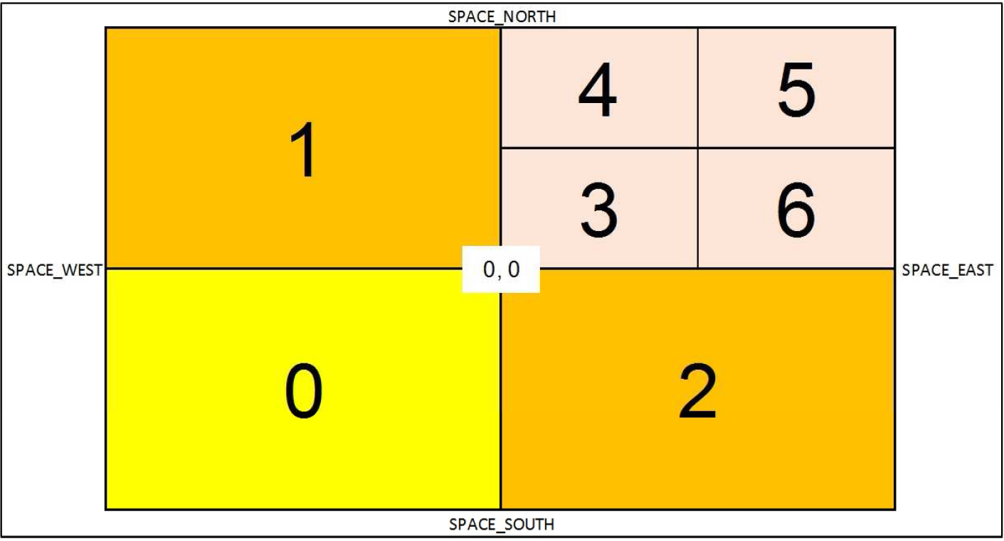
Three different designs were used and are applied by changing the number of regions \(\eta\). If \(\eta\) is equal to 1, the model runs with only one region, with code 0, which encompasses the entire space. When \(\eta\) is equal to 4, the model runs with four regions, with codes 0, 1, 2 and 3, and region 3 covers the entire area of subregions 3, 4, 5 and 6 in Figure 1. Finally, with seven regions, the model follows the configuration of the codes of Figure 1, with four smaller regions and three larger ones.
Model implementation and parameters
Running the model is simple and done with just one command. Optionally, the modeler can set the parameters for each simulation and for the run itself, as described below. A systematic analysis of the parameters that assesses whether small changes significantly affect the results and seek to confirm the robustness of the model (sensitivity analysis) is made after the presentation of results.
For each simulation run you can choose the number of agents, families, households, the time duration in days, the number of local governments in which space is divided (namely, municipalities, with competence over their territory) and the path file to save the results (Table 2).
| Simulation parameters | Values | Possibilities’ intervals | Observations |
|---|---|---|---|
| Number of days | 5,040 | (63 - 12,800) | The model was developed to run up to 50 years, however with loss of explanatory power. We ran the model for 20 years |
| Number of agents | 1,000 | (10 - 10,000) | Increasing the number of agents makes the simulation slower |
| Number of families | 400 | (4 - 2,000) | Used to define the average number of agents per family. The suggestion is to have 2.5 agents per family, on average |
| Number of dwellings | 440 | (5 - 2,200) | Necessarily higher than the number of families. Vacancy in Brazil is around 11% |
| Number of firms | 110 | (2 - 1,000) | Approximately 10% of the number of agents |
| Number of regions | 1- 4 - 7 | (1 - 4 - 7) | Alternative number of regions to run the model |
| Model parameters | |||
| Firms | |||
| Alpha | 0.25 | (0 - 1) | Production function exponent. When set to ”1”, it does not change the model, when set to ”0”, the production of the firm is one unit |
| Beta | 0.87 | (0 - 1) | Consumption function exponent. When set to ”1” consumption vary from zero to the total of available money |
| Quantity to change prices (∂) | 10 | (100 - 2,000) | Threshold to change prices |
| Frequency of entrance in labor market | 0.28 | (0 - 1) | Time frequency of decision-making on labor market. When set to “0”, the evaluation is made every month. When set to “0.25”, the firm enters the market three times every four months, on average |
| Mark-up | 0.03 | (0 - 1) | Percentage added to prices when demand is high (product level on inventory is below ”Quantity to change prices”) |
| Agents | |||
| Labor market size (Γ) | 100 | (1 - 1,000) | Number of firms checked before agents make decision to consume. Can be set between ”1” and the total number of firms |
| Consumption satisfaction | 0.01 | [0 - 1) | Used to measure satisfaction gained with consumption |
| Families | |||
| Real estate market | 0.021 | (0 - 1) | Percentage of families’ entering real estate market |
| Government | |||
| Consumption tax | 0.21 | (0 - 1) | Tax on consumption |
The proposed model contains a very small number of exogenous parameters. The parameters help understand how the model mechanisms influence its results. Parameter \(\alpha\), for example, can be set to 1 so that its effect is zero. By reducing the parameter successively by 0.1, one can observe the effect of increasingly less productive workers. The same understanding of relevance can be made with the \(\beta\) parameter, or the rate of consumption tax. This construction offers some flexibility to the modeler. This flexibility is most relevant if the goal is to increase understanding of the problem that is modeled and the model is used as a guiding tool for decision-making, or as a methodology to discuss “what if” questions.
Limitations
The limitation of this study arises from the difficulty of finding complete, integrated, and simple models that could be used as initial steps to be expanded and adapted by following researchers. In fact, apart from the models of Lengnick (2013) and Gaffeo et al. (2008), all others are specific to a single market, such as energy (Koesrindartoto, Sun, & Tesfatsion 2005), finance (Feng et al. 2012) or labor market (Seppecher 2012); or are too complex (Dawid et al. 2014; Van Der Hoog et al. 2008).
Another question raised by the choice of a ‘simple’ model is of an epistemological nature. How can we determine which are the central elements of the phenomenon, which must be present, and what are the accessory elements? At what point, simplifying the process can take place and where there is significant change of the observed phenomenon?
Besides this general limitation, this version of the model also does not include the credit market, demographic changes nor investment in social capital.
Results and discussion
The results indicate that – for the given configuration, and considering 1,000 iterations – the real estate market is dominant for the results. The fact that price is given partially by the quality of life index (QLI) of the region leads to increase in prices in those regions with better QLI. Simultaneously, families that are on average worse off use such price difference to capitalize, selling their valued-home and moving to suburbs with worse QLI. Thus, the model with seven regions benefits from higher levels of cash in the hands of the families, which leads to higher consumption, production and GDP. All these factors together in turn promotes higher inequality.
Consumption determines the labor market behavior. Consumption is higher both when the propensity to consume (beta) or the families’ wealth is at high levels. Therefore, when firms are selling well, they make quarterly profits and keep hiring in order to increase productivity. The goods market is dependent mainly on consumers’ decision to purchase, as the productivity of workers – given by their qualification – is usually enough to provide the firm with high levels of products in stock. The firms’ hiring capacity is also fast enough to respond to increase in demands.
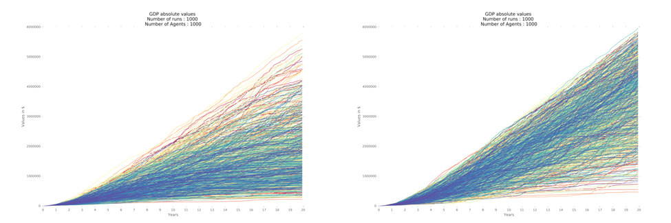
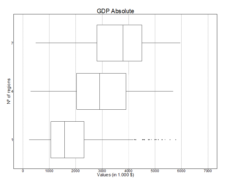
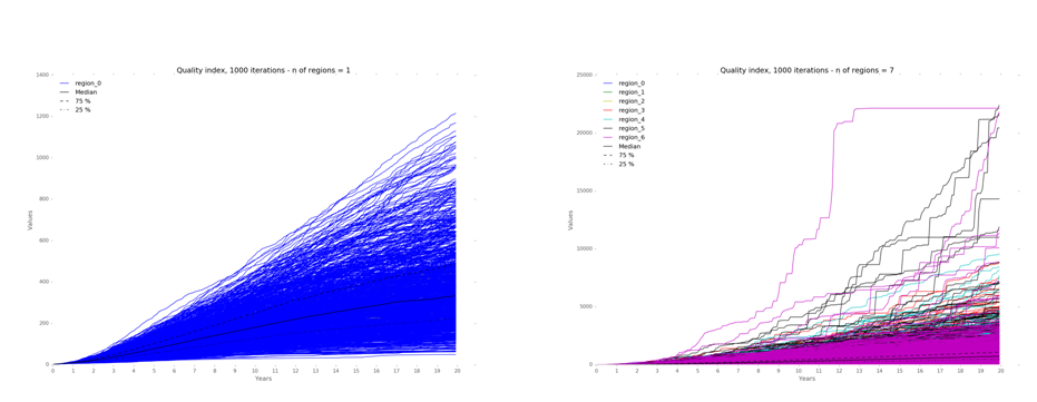
The most thriving economy is the model with seven regions (Figure 2), on average with median GDP 30% higher when compared to the model with four regions. The model with four regions, in turn, achieves results that are 38% above the model with a single region (Table 3). The variability is higher for the model with seven regions, vis-à-vis the model with one region (Figure 3).
| Regions | 0.25 | Median | 0.75 | |
|---|---|---|---|---|
| GINI | 1 | 0.890 | 0.916 | 0.932 |
| 4 | 0.925 | 0.939 | 0.946 | |
| 7 | 0.935 | 0.944 | 0.950 | |
| GDP | 1 | 1,056,341 | 1,568,746 | 2,314,751 |
| 4 | 2,029,562 | 2,904,486 | 3,897,685 | |
| 7 | 2,794,786 | 3,788,903 | 4,501,469 | |
| QLI | 1 | 223.21 | 331.79 | 487.26 |
| 4 | 425.02 | 608.90 | 820.88 | |
| 7 | 562.13 | 761.78 | 945.87 | |
| Families’ wealth | 1 | 589.0 | 19,757.1 | 115,814.6 |
| 4 | 32,126.4 | 253,449.6 | 893,763.6 | |
| 7 | 82,189.9 | 573,573.3 | 1,645,295.6 |
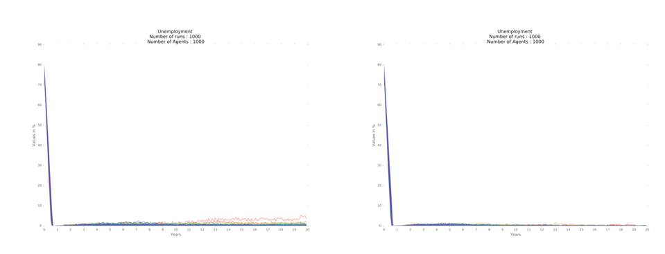
Considering the labor market, the economies converge towards full employment, keeping a cycle of very .low unemployment, throughout the period, for the three regional designs show similar results (Figure 4).
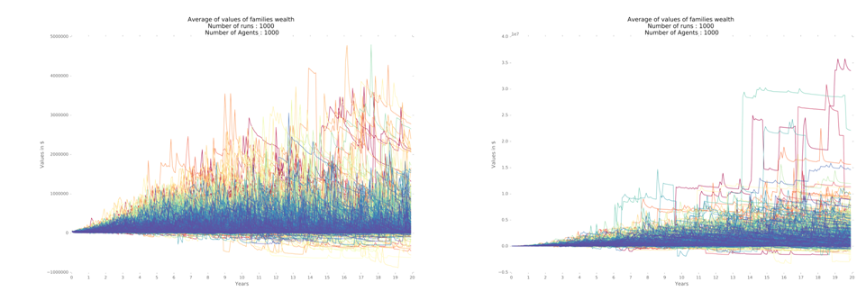
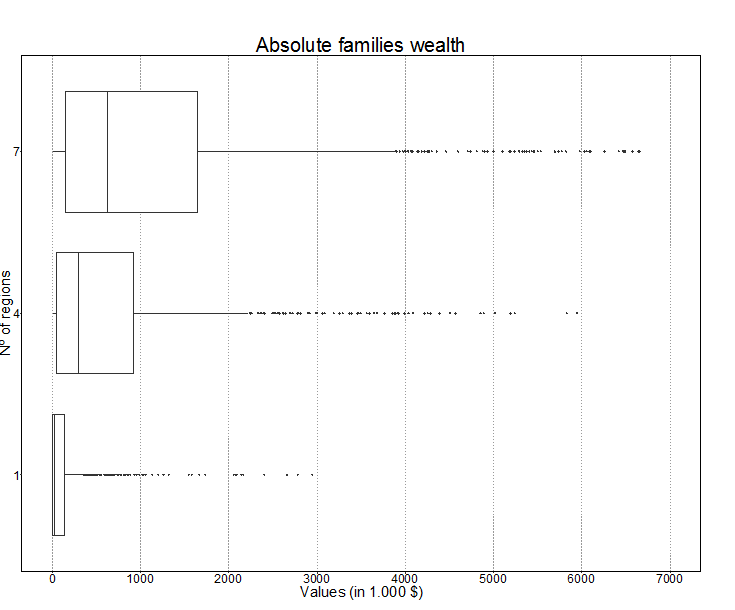
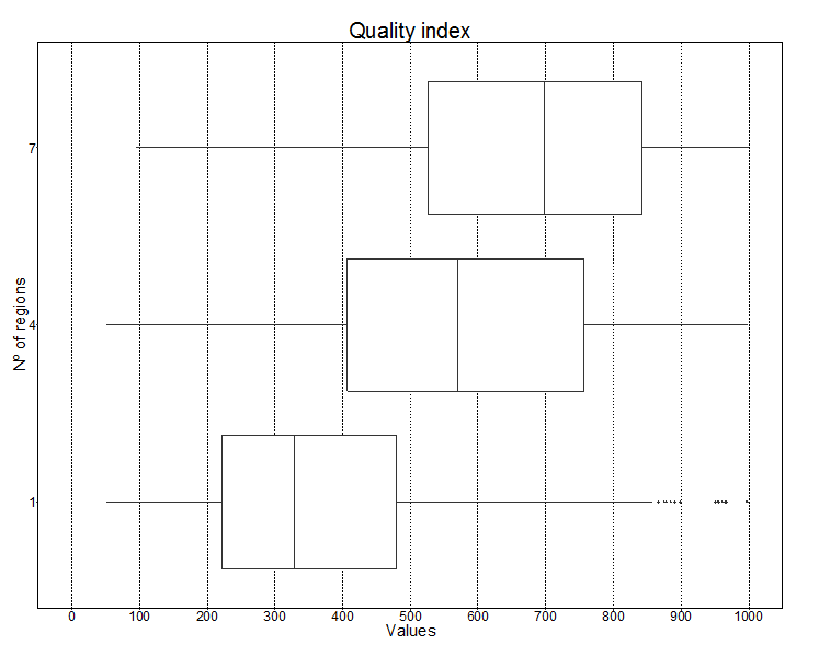
Household income varies significantly among the three regional designs, for one region variation is of lower magnitude when compared to seven regions (Figure 5) through 1,000 iterations. The median, first and third quartiles are higher for the model with seven regions, vis-à-vis the model with only one region (Table 3 and Figure 6).
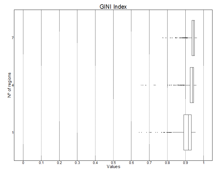
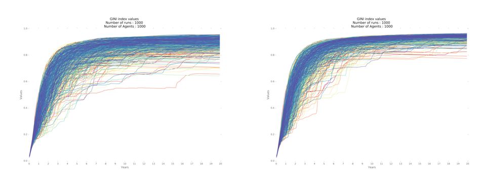
The Gini coefficient is computed on the utility of the families. Utility is directly proportional to the cumulative consumption of the families. The GINI coefficient reaches a higher level in the model with 7 regions when compared to the two other models (Figure 7). Moreover, the behavior of the coefficient in the 1,000 iterations has a similar pattern of variability with slightly higher standard deviation (Figure 8). Hence, it confirms the greater inequality among families in the model with 7 regions.
Finally, the basic indicator to compare the performance of the models is the Quality of Life Index for each simulated design for one region and for seven regions (Figure 9). The median and the first and third quartiles are higher for the model with seven regions vis-à-vis the other models (Figure 10).
The model results indicate that changes in administrative boundaries have led to robust changes among the three considered region design. According to the procedures described, the dynamism of the real estate market, namely, household mobility in the simulations with more than one region, was relevant to the results.
In the absence of a credit market, families with income level below the median become sellers in the real estate market. Thus, these families capitalize on the sale of homes whose prices increased along with the quality of life in the region, and migrate toward regions with poorer quality. This movement is partly counterbalanced by families trying to migrate in search of better quality. As a result, the models with subdivisions lead to regions that are less populated and have better quality of life and at the same time, more populated regions that have worse QLI.
It is noteworthy the tradeoff between the results for the three models. While the model with seven regions is more dynamic, more productive and wealthier, it is also more heterogeneous. The model with one region, in turn, is more harmonic but less vigorous (Table 4).
The underlying assumption of the authors – that the model with one region would be more efficient from the standpoint of conurbation regions – was not observed with the present configuration. Especially given the strength and mobility of the real estate market that concentrates smaller populations in regions with higher quality and larger populations in areas with poorer quality. However, the research question – that is, if administrative boundaries influence the economic and fiscal dynamic of the regions – can be confirmed. Yet, the results indicate the wealth of possibilities of analysis of the economic system from heterogeneous agents and firms in an environment that is continually changing.
Finally, given the process of creating artificial economies, at each loop iteration the agents and firms are completely different. Thus, the next phase of research, which is the model application to real data, will input actual data as attributes of the economy and thus reduce the variability of results.
| Regions | QLI median | QLI sd. | |
|---|---|---|---|
| 1 | Max | 333.5 | 210.9 |
| Min | 333.5 | 210.9 | |
| 4 | Max | 860.2 | 430.2 |
| Min | 423.2 | 198 | |
| 7 | Max | 1,499.2 | 2,047.7 |
| Min | 343.9 | 195.3 |
Sensitivity analysis and robustness – the influence of consumption taxes
The sensitivity analysis is central in building simulation models to ensure that the model is structurally consistent and does not depend solely on a particular parameter, which is adjusted for a specific value. Furthermore, the sensitivity analysis may serve as an analytical tool to show how and with which magnitude certain configurations and model processes change trends and results.
The sensitivity analysis made was based on the variation of the model parameters in 10 different values between their minimum and maximum values (Table 5). As random numbers influence the model results, comparing the results of different iterations (model runs) is only possible if we use the same seed. Thus, if the model is run several times with the same parameter and the same seed, the same results will be produced. Therefore, when the modeler changes the parameters, variations in sensitivity analysis results will be a result of the model structure and not of the random number generator13.
The change of the parameters was performed separately (one parameter at a time) with the other parameters maintained at their default values, defined in a first exploratory analysis.
Given that the premise is to create a model (or simulation machine), the sensitivity analysis furthers our understanding of the model. Here we present the sensitivity analysis for the variation of the value on consumption tax. An appendix presents variations on alpha, beta and other parameters. Of course, we also varied the number of regions (1, 4, 7).
| Parameters | Values | |||||||||
|---|---|---|---|---|---|---|---|---|---|---|
| Alpha | 0.1 | 0.14 | 0.19 | 0.23 | 0.28 | 0.32 | 0.37 | 0.41 | 0.46 | 0.5 |
| Beta | 0.5 | 0.55 | 0.61 | 0.66 | 0.72 | 0.77 | 0.83 | 0.88 | 0.94 | 0.99 |
| Quantity to change prices | 10 | 42.2 | 74.4 | 106.7 | 138.9 | 171.1 | 203.3 | 235.6 | 267.8 | 300 |
| Markup | 0.01 | 0.04 | 0.06 | 0.09 | 0.12 | 0.14 | 0.17 | 0.2 | 0.22 | 0.25 |
| Labor market entry | 0.1 | 0.14 | 0.19 | 0.23 | 0.28 | 0.32 | 0.37 | 0.41 | 0.46 | 0.5 |
| Market size | 10 | 21 | 32 | 43 | 54 | 65 | 77 | 88 | 99 | 110 |
| Real estate entry | 0.01 | 0.02 | 0.03 | 0.04 | 0.05 | 0.06 | 0.07 | 0.08 | 0.09 | 0.1 |
| Tax consumption | 0.01 | 0.06 | 0.11 | 0.16 | 0.21 | 0.25 | 0.3 | 0.35 | 0.4 | 0.45 |
Tax on consumption
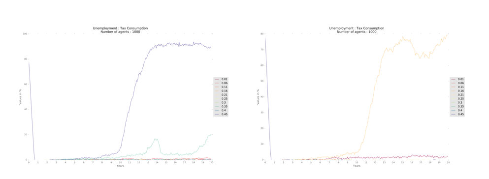
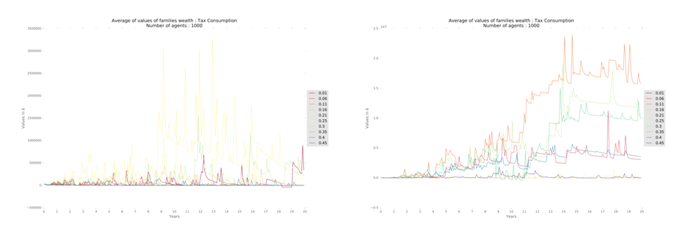
The value of the tax rate influences the economy on many levels. Lower rates lead to lower unemployment, but influence little when below 0.3 (Figure 11). High tax rates bring hyperinflation, widespread unemployment and a significant drop in revenues and profits of firms. However, given that the amounts collected in taxes are applied in the same regions where were collected, QLI improves, and consequently, property prices increase accordingly. Household income (Figure 12) and GDP are higher for intermediate values of tax rate.
Thus, we understand that the variation of the results of the model given by the variation of the parameters is in line with the underlying literature. In addition, there is no change of parameters that cause different or unexpected behavior of the model. Hence, we believe it indicates the robustness of the model, as described.
The methodological approach: possibilities for future research
This section describes various additions to the model that could be implemented with relatively small and simple changes in the current code. Given the seminal methodological trait of this paper, we thought the model should be developed in its simplest form possible, following the KISS logic (‘keep it simple, stupid’). Eventually, it could evolve into the KIDS form (‘keep it descriptive, stupid’), formulated by Edmonds and Moss (2005).
The immediate interest of the authors, it is to apply it for the Federal District region, in Brazil. Empirical data would be used in the initial configuration of the model, namely: actual municipal boundaries, specific spatially-bound demographic patterns, actual companies attributes and location, and supply of skilled labor. The following step would be to validate the empirical model for a given timeline, seeking correlation or similarity between the evolution of observed indicators and those produced by the model. Finally, after validation, the model could be effectively used to implement public policy alternatives.
The actual realm of research possibilities are detailed below, following the KIDS argument of Edmonds and Moss (2005).
- Implement demographic change, with processes that describe birth, deaths and families’ creation in order to become a more dynamic and real model while enabling results for specific demographic cohorts. In addition, inter-temporal analyzes involving inheritance (of wealth or social capital), could also be tested.
- Another relatively simple alternative is the inclusion of updating workers qualification (years of study), deducing investment from their resources.
- The credit market, with production and consumer financing possibility is also relevant to make the model closer to economic reality. The literature is already available (Cajueiro & Tabak 2005, 2008; Tabak et al. 2009)
- Currently, the market for goods is restricted to firms and consumers in the domestic market. However, it could also include firms and governments as buyers (and sellers), enabling analysis of intermediate sectors, as well as foreign buyers allowing the inclusion of an economic measure of exports and trade balance.
- Although distance is already included in the model, the formula could be sophisticated to effectively include the transport system available in the municipalities that are object of study. As a result, accessibility analysis would be systematically integrated with the rest of the economy, as demand and supply of the transport system (for employment purposes).
- The process of imposing a limit by time or distance to daily commute would endogenously enable the creation of a system with several regions, making it simple to study urban hierarchy analysis. In such case, the ‘employment areas’ would be endogenous to the model.
- Firms and their production technologies, decision-making processes and hiring and firing could be drawn from tacit information specific to a particular firm or sector.
- The taxation system of this model is simplistic, with only one tax applied to consumption, typically a value-added tax (VAT) levied on the location of the firm. However, note the reader, that the implementation of the Territorial Taxes on property or on income, or changing VAT to be collected at the destination, i.e., at the consumer’s place of residence, could be easily implemented. Thus, specific research questions of fiscal interest could be investigated.
- Implementation of item 8 would also enable the analysis of the dynamics of taxes across neighboring municipalities with different tax policies.
Indeed, it is worth mentioning the advantage of modularity within the scope of this work. Using the basic model is possible to detail, build, and expand the model module by module, according to the research needs, while ensuring the evolution of the integration of other processes already implemented and validated. Anyway, this list is not exhaustive and only fulfills the job of informing the model expansion opportunities, through enhanced feature of this theoretical and methodological proposal.
Final Considerations
This paper specifies, explains and justifies the steps and processes of the construction of the computational algorithm that prospectively simulates a spatial economy. It adds to the literature (a) on the explicit spatiality of the model, and (b) in achieving a simple model with three markets and conurbated subnational governments. Thus, the model establishes an actual framework for economic simulation and it constitutes itself as a public policy tool.
The model has a dynamic real estate market with prices given by the features of the dwelling and its location; a labor market, with matching mechanism between skilled workers and companies; and a goods market with endogenous price adjustment based on stock. The configuration in different subnational governments, one, four or seven differentiated regions allows for explicit spatial analysis.
The results and trends obtained after 1,000 simulation runs indicate that mobility of families among regions is central to the model with impoverished families migrating to poorly serviced places and, therefore, lower real estate prices; and families that are financially well migrating to better quality areas. Therefore, the model with only one region has a less dynamic economy, although more homogeneous, whereas the model with seven regions shows greater dynamism, but also greater heterogeneity and inequality.
Moreover, it is important to highlight that the results of the model reflect observed behavior for Brazilian metropolises. That is, higher quality of life areas get expensive as public services accumulate. Such increase in prices push people towards areas with lower quality of life, but that are more affordable. Thus, places with low QLI become more populated and those with high QLI have sparser population.
The research question that asked whether the change of administrative boundaries and the consequent change of local tax revenue dynamics, in principle, changes the quality of life of the citizens ‘can be answered affirmatively. Indeed, administrative boundaries – understood as enclosed area of tax collection over economic base and its investment as collective public services – can alter the quality of life of citizens.
The underlying question faced by this paper is the efficiency of the return of taxes to taxpayers. Is there a spatial, political and administrative configuration that is more efficient? This debate should be further discussed by following research.
Finally, this paper contributes to the methodological framework of economic tools, particularly those flexible and forward-looking, with applied realm to public policies of subnational entities.
Acknowledgements
We would like to thank the National Council of Research (CNPq) for their support.Notes
- This concept is detailed in the description of the model, section 2.
- See Pinto's (2014, p.75) discussion: “The decentralization and fragmentation of the territory poses alternatives for consumers of collective services who cannot buy services individually, but may buy a package of services and goods that are more preferable”.
- For a more detailed review, see Winikoff et al. (2012).
- Upon publication, the code will be made available in GitHub and OpenABM.
- For an introduction in Python, see Downey (2012).
- The number of dwellings should always be larger than the number of families, for this version of the model.
- That is, properties prices are defined by their own features, plus local attributes.
- Adapted from Dosi et al. (2009) and Lengnick (2013).
- Bergmann (1974) uses cost and profit information in addition to stock levels to determine price changes. Dawid et al. (2012) use stock levels to define production quantity.
- For this specification, k was set to 0.65.
- We have calculated the bias via a bootstrapping procedure. After 10,000 simulations – given workers' schooling varying from one to 20 years of study – the selected worker had more than 15 years of study in half of the times; more than 10 years of study 75% of the times and above 7 in 90% of the times.
- Neugart et al. (2012) have discussed matching mechanisms for the labor market but ponder that there is insofar no consensus about the best procedure.
- The results of the sensitivity analysis were obtained using a fixed seed.
Appendix: Sensitivity analysis
Alpha
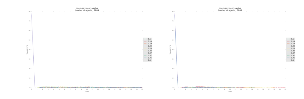
The variation of each of the parameters affects differently the results of the simulations. The alpha parameter – which evaluates worker productivity – for example, leads to higher values of total GDP when values are between .32 and 0.37.
Considering unemployment, the alpha parameter provides full employment, conditioned to the other parameter’s default values. Figure 13 shows that unemployment converges quickly towards full employment. The behavior was similar for all regions.
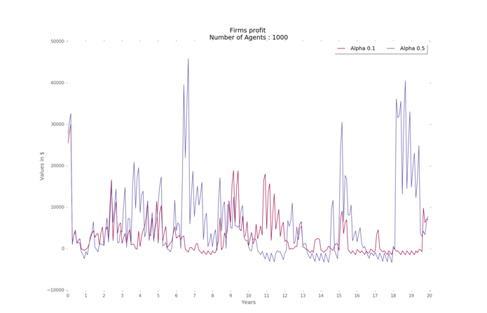
The variation in productivity and unemployment indicate that when worker productivity is very high, there is an excess supply that is not absorbed by the market. However, there is greater variation in firms’ profits when alpha is higher and slightly more stability at lower levels when alpha is smaller (Figure 14). The value of alpha at 0.25 results in a good balance of resources in the economy among firms and households, on average, for all the region designs. Finally, the Gini coefficient is slightly higher for higher values of alpha.
Beta
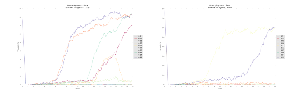
The beta parameter – which controls the propensity to consume of households – heavily influences the economy. In fact, higher values of beta (lower discount at maximum limit of household spending) or lower levels of beta, which restricts consumption, lead to high and persistent levels of unemployment (Figure 15), especially in the model with one region, where the dynamics is more dependent on the goods market.
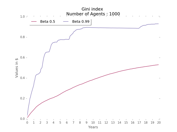
Low values also keep firms’ profits close to zero. The impact of beta in the Gini coefficient is relevant and similar among the regional designs used. For low values of beta and low household consumption, Gini rises gradually, reaching a maximum at about 0.50. However, when beta has a value of 0.99, inequality rises steeply to reach values close to 0.90 at the end of the period (Figure 16).
Other parameters
A sensitivity analysis was performed for each exogenous parameters of the model, with lower relative impact compared to parameters alpha, beta and the tax rate. The level of the inventory that influences prices seem to impact little in prices, except for higher levels. The frequency with which firms enter the labor market affects the speed of adjustment in the labor market. When parameter values are higher – taking longer to enter the labor market – unemployment is only insignificant at the end of the period. When the entry of firms is frequent, full employment is achieved within months. The change in the markup value, i.e., the percentage increase in product prices of firms when their stock is low – does not greatly change the profit levels of the firms. However, very high mark-up rates, lead to uncontrolled inflation after some time. The size of the market checked by consumers when they go shopping interferes only marginally in the results. Finally, the percentage of families entering the housing market seems to have little influence. When all families are on the market all the time, there is a small reduction in household income.
References
ADAMATTI, D. F., Sichman, J. S., & Coelho, H. (2009). An analysis of the insertion of virtual players in GMABS methodology using the vip-Jogoman prototype. Journal of Artificial Societies and Social Simulation, 12(3), 7: https://www.jasss.org/12/3/7.html.
AFONSO, A., Romero, A., & Monsalve, E. (2013). Public Sector Efficiency: Evidence for Latin America (IDB Publications No. 80478). Inter-American Development Bank.
AFONSO, J. R. R. (2014). Imposto de renda e distribuição de renda e riqueza: as estatísticas fiscais e um debate premente no Brasil. Revista da Receita Federal: estudos tributários e aduaneiros, 1(1), 28–60.
ANDERSON, P. W., Arrow, K., & Pines, D. (1988). The economy as an evolving complex system. In The Proceedings of the Evolutionary Paths of the Global Economy Workshop. Santa Fe, NW.
ANDRADE, L. T., & Figueiredo, F. O. V. de. (2005). Vulnerabilidade social e criminalidade na Região Metropolitana de Belo Horizonte. In XII Congresso Brasileiro de Sociologia (p. 19).
ANTINARELLI, M E. P. B. (2012). Federalismo, autonomia municipal e a constitucionalização simbólica: uma análise da dependência financeira dos pequenos municípios mineiros. Revista Da Faculdade de Direito Da UFMG, (61), 445–472.
ARNOTT, R. (1987). Economic theory and housing. In Handbook of Regional and Urban Economics (p. 959–988). Amsterdam: Elsevier Science Publishers.
ARTHUR W. B. (1994) Inductive Reasoning and Bounded Rationality. The American Economic Review, 84(2), 406–411.
AXELROD, R., & Hamilton, W. D. (1981). The evolution of cooperation. Science, 211(4489), 1390–1396. [doi:10.1126/science.7466396]
BAHL, R. (2010). Financing metropolitan areas. In Local government finance (pp. 309–335). Barcelona: UCLG - United Cities and Local Governments.
BARGIGLI, L., & Tedeschi, G. (2014). Interaction in agent-based economics: A survey on the network approach. Physica A: Statistical Mechanics and its Applications, 399, 1–15. [doi:10.1016/j.physa.2013.12.029]
BERGMANN, B. R. (1974). A microsimulation of the macroeconomy with explicitly represented money flows. In Annals of Economic and Social Measurement, Volume 3, number 3 (p. 475–489). NBER.
BLINDER, A. S. (1982). Inventories and sticky prices. The American Economic Review, 334–48.
BLINDER, A. S. (1994). On sticky prices: academic theories meet the real world. In Monetary policy (p. 117–154). The University of Chicago Press: N. Gregory Mankiw.
BOERO, R., Morini, M., Sonnesa, M., & Terna, P. (2015). Agent-based models of the economy: from theories to applications. Palgrave Macmillan. [doi:10.1057/9781137339812]
BOUDREAU, J. W. (2010). Stratification and growth in agent-based matching markets. Journal of Economic Behavior & Organization, 75(2), 168–179. [doi:10.1016/j.jebo.2010.03.021]
BRANDALISE, L. T., Rojo, C. A., da Mata, D. M., & de Souza, A. F. (2012). Simulação de cenários e formulação de estratégias competitivas: o caso do atacado liderança. Revista Gestão & Tecnologia, 12(3), 223–257.
BRUECKNER, J.K. (1987). The structure of urban equilibria: a unified treatment of the Muth-Mills model (Handbook of Regional and Urban Economics). New York, NY: E.S. Mills.
CAJUEIRO, D. O., & Tabak, B. M. (2005). Possible causes of long-range dependence in the Brazilian stock market. Physica A: Statistical Mechanics and its Applications, 345(3), 635–645. [doi:10.1016/S0378-4371(04)01005-2]
CAJUEIRO, D. O., & Tabak, B. M. (2008). The role of banks in the Brazilian Interbank Market: Does bank type matter? Physica A: Statistical Mechanics and its Applications, 387(27), 6825–6836.
CANUTO, O., & Liu, L. (2013). Until debt do us part: Subnational debt, insolvency, and markets, World Bank Publications. [doi:10.1596/978-0-8213-9766-4]
CARLEY, K. M. (1996). Validating computational models. Carnegie Mellon University, p.40 (mimeo).
CARVALHO, G., Oliveira, A., & Oliveira, C. (2015). Cenários de longo prazo para a cafeicultura brasileira: 2006-2015. SOBER Proceedings.
CIARLI, T. (2012). Structural Interactions and Long Run Growth. Revue de l’OFCE, 124(5), 295–345. [doi:10.3917/reof.124.0295]
DAVID, N., Sichman, J. S., & Coelho, H. (2005). The logic of the method of agent-based simulation in the social sciences: Empirical and intentional adequacy of computer programs. Journal of Artificial Societies and Social Simulation, 8(4) 2: https://www.jasss.org/8/4/2.html
DAWID, H., Gemkow, S., Harting, P., & Neugart, M. (2012). Labor market integration policies and the convergence of regions: the role of skills and technology diffusion. Journal of Evolutionary Economics, 22(3), 543–562. [doi:10.1007/s00191-011-0245-1]
DAWID, H., Gemkow, S., Harting, P., Van der Hoog, S., & Neugart, M. (2014). Agent-based macroeconomic modeling and policy analysis: the Eurace@Unibi model. Bielefeld Working Papers in Economics and Management.
DIPASQUALE, D., & Wheaton, W. C. (1996). Urban economics and real estate markets. Englewood Cliffs, NJ: Prentice Hall.
DOSI, G., Fagiolo, G., Napoletano, M., & Roventini, A. (2012). Income Distribution, Credit and Fiscal Policies in an Agent-Based Keynesian Model. SSRN eLibrary. [doi:10.2139/ssrn.1990209]
DOSI, G., Fagiolo, G., & Roventini, A. (2009). The microfoundations of business cycles: an evolutionary, multi-agent model. In U. Cantner, J.-L. Gaffard, & L. Nesta (Orgs.), Schumpeterian Perspectives on Innovation, Competition and Growth (p. 161–180). Springer Berlin Heidelberg. [doi:10.1007/978-3-540-93777-7_10]
DOWNEY, A. (2012). Think Python. United States of America: O’Reilly Media.
EDMONDS, B., & Moss, S. (2005). From KISS to KIDS–an “anti-simplistic” modelling approach. In Multi-Agent and Multi-Agent-Based Simulation, Volume 3415, Lecture Notes in Computer Science, pp 130-144, Springer. [doi:10.1007/978-3-540-32243-6_11]
ELIASSON, G., Olavi, G., & Heiman, M. (1976). A Micro-Macro Interactive Simulation Model of the Swedish Economy: Preliminary Model Specification. IUI Working Paper.
EPSTEIN, J. M., & Axtell, R. (1996). Growing artificial societies: social science from the bottom up. Cambridge, MA: Brookings/MIT Press.
FENG, L., Li, B., Podobnik, B., Preis, T., & Stanley, H. E. (2012). Linking agent-based models and stochastic models of financial markets. Proceedings of the National Academy of Sciences, 109(22), 8388–8393. [doi:10.1073/pnas.1205013109]
FUJITA, M., Krugman, P., & Venables, A. (1999). The spatial economy: cities, regions and international trade. Cambridge, Mass.: MIT Press.
FURTADO, B., Mation, L., & Monasterio, L. (2013). Fatos estilizados das finanças públicas municipais metropolitanas brasileiras entre 2000-2010. In Território metropolitano, políticas municipais (p. 291–312). Brasília: Furtado, Bernardo; Krause, Cleandro; França, Karla.
GAFFEO, E., Delli Gatti, D., Desiderio, S., & Gallegati, M. (2008). Adaptive microfoundations for emergent macroeconomics. Eastern Economic Journal, 34(4), 441–463. [doi:10.1057/eej.2008.27]
GASPARINI, C. E., & Miranda, R. B. (2011). Transferências, equidade e eficiência municipal no Brasil. Planejamento e Políticas Públicas, (36).
GOBETTI, S. W. (2015). Ajuste fiscal no Brasil: os limites do possível. Textos para Discussão, 2037.
GRILLI, R., Tedeschi, G., & Gallegati, M. (2014). Markets connectivity and financial contagion. Journal of Economic Interaction and Coordination, 1–18.
GRIMM, V., Berger, U., Bastiansen, F., Eliassen, S., Ginot, V., Giske, J., et al. (2006). A standard protocol for describing individual-based and agent-based models. Ecological modelling, 198(1), 115–126. [doi:10.1016/j.ecolmodel.2006.04.023]
GRIMM, V., Berger, U., DeAngelis, D. L., Polhill, J. G., Giske, J., & Railsback, S. F. (2010). The ODD protocol: a review and first update. Ecological Modelling, 221(23), 2760–2768. [doi:10.1016/j.ecolmodel.2010.08.019]
GUOCHENG, W., Yuna, S., Jie, W., & Zili, W. (2015). Application analysis on large-scale computation for social and economic systems. International Conference on Systems, Man and Cybernetics, Hong Kong: IEEE SMC.
HASSAN, S., Pavón, J., Antunes, L., & Gilbert, N. (2010). Injecting data into agent-based simulation. In Simulating Interacting Agents and Social Phenomena (p. 177–191). Springer. [doi:10.1007/978-4-431-99781-8_13]
HOLLAND, J. (1992). Complex adaptive systems. Daedalus, 121, 17–30.
HOLLAND, J., & Miller, J. H. (1991). Artificial Adaptive Agents in Economic Theory. The American Economic Review, 81(2), 65–71.
KOESRINDARTOTO, D., Sun, J., & Tesfatsion, L. (2005). An agent-based computational laboratory for testing the economic reliability of wholesale power market designs. In Power Engineering Society General Meeting, 2005. IEEE (p. 2818–2823). IEEE. [doi:10.1109/PES.2005.1489273]
LeBARON, B. (2006). Agent-based Computational Finance (Vol. 2, p. 1187–1233). Elsevier.
LeBARON, B., & Tesfatsion, L. (2008). Modeling macroeconomies as open-ended dynamic systems of interacting agents. The American Economic Review, 246–250. [doi:10.1257/aer.98.2.246]
LENGNICK, M. (2013). Agent-based macroeconomics: A baseline model. Journal of Economic Behavior & Organization, 86, 102–120. [doi:10.1016/j.jebo.2012.12.021]
LÖSCH, A. (1954). The economics of location. New Haven: Yale University Press.
MANKIW, N. G. (2011). Principles of Economics, (6 ed.). South-Western College Pub.
MAROULIS, S., Bakshy, E., Gomez, L., & Wilensky, U. (2010). An agent-based model of intra-district public school choice. Northwestern University Working Papers, 30.
MAROULIS, S., Bakshy, E., Gomez, L., & Wilensky, U. (2014). Modeling the transition to public school choice. Journal of Artificial Societies and Social Simulation, 17(2) 3: https://www.jasss.org/17/2/3.html [doi:10.18564/jasss.2402]
MIDGLEY, D., Marks, R., & Kunchamwar, D. (2007). Building and assurance of agent-based models: An example and challenge to the field. Journal of Business Research, 60(8), 884–893. [doi:10.1016/j.jbusres.2007.02.004]
NADALIN, V. G. (2010). Três ensaios sobre economia urbana e mercado de habitação em São Paulo (tese de doutorado). IPE-USP, São Paulo.
NARDIN, L. G., & Sichman, J. S. (2012). Trust-based coalition formation: A multiagent-based simulation. In Proceedings of the 4th World Congress on Social Simulation.
NEUGART, M., Richiardi, M., et al. (2012). Agent-based models of the labor market. LABORatorio R. Revelli working papers series, 125.
OATES, W. E. (1972). Fiscal Federalism. New York: Harcourt Brace.
OATES, W. E. (1999). An Essay on Fiscal Federalism. Journal of Economic Literature, 37 (3): 1120–49. [doi:10.1257/jel.37.3.1120]
OLSON, M. (1969). The Principle of ‘Fiscal Equivalence’: The Division of Responsibilities among Different Levels of Government. The American Economic Review 59 (2): 479–87.
ORAIR, R. O., Santos, C. H. M., Silva, W. de J., Brito, J. M. de M., Ferreira, A. dos S., Silva, H. L., & Rocha, W. S. (2011). Uma metodologia de construção de séries de alta frequência das finanças municipais no Brasil com aplicação para o IPTU e o ISS: 2004-2010. Pesquisa e Planejamento Econômico, 41(3), 471–508.
PALMER, Rg., Brian Arthur, W., Holland, J. H., LeBaron, B., & Tayler, P. (1994). Artificial economic life: a simple model of a stockmarket. Physica D: Nonlinear Phenomena, 75(1), 264–274. [doi:10.1016/0167-2789(94)90287-9]
PINTO, V. C. (2014). Direito Urbanístico - Plano Diretor e Direito de Propriedade. Revista dos Tribunais.
REZENDE, F. (2010). Federalismo Fiscal: em busca de um novo modelo. In Educação e federalismo no Brasil: combater as desigualdades, garantir a diversidade (p. 71–88). Brasília: Unesco.
REZENDE, F. & Garson, S. (2006). Financing metropolitan areas in Brazil: Political, institutional and legal obstacles and emergence of new proposals for improving coordination. Revista de Economia Contemporanea, 10(1): 5-34. [doi:10.1590/S1415-98482006000100001]
SANTOS, C. H. M. dos O., & Gouvêa, R. R. O. (2014). Finanças públicas e macroeconomia no Brasil: um registro da reflexão do Ipea (2008-2014). Brasília: IPEA.
SCHELLING, T. C. (1969). Models of segregation. The American Economic Review, 488–493.
SCHETTINI, B. P., dos Santos, C. H. M., Amitrano, C. R., Squeff, G. C., Ribeiro, M. B., Gouvêa, R. R. (2012). Novas evidências empíricas sobre a dinâmica trimestral do consumo agregado das famílias brasileiras no período 1995-2009. Economia e Sociedade, 21(3), 607–641. [doi:10.1590/S0104-06182012000300006]
SEPPECHER, P. (2012). Flexibility of wages and macroeconomic instability in an agent-based computational model with endogenous money. Macroeconomic Dynamics, 16(S2), 284–297. [doi:10.1017/S1365100511000447]
STRAATMAN, B., Marceau, D. J., & White, R. (2013). A generic framework for a combined agent-based market and production model. Computational Economics, 41(4), 425–445. [doi:10.1007/s10614-012-9341-z]
TABAK, B. M., Cajueiro, D. O., & Serra, T. R. (2009). Topological properties of bank networks: the case of Brazil. International Journal of Modern Physics C, 20(08), 1121–1143. [doi:10.1142/S0129183109014205]
TESFATSION, L. (2006). Agent-Based Computational Economics: A Constructive Approach to Economic Theory. In Handbook of Computational Economics (Vol. 2, p. 831–880). Elsevier. [doi:10.1016/S1574-0021(05)02016-2]
TIEBOUT, C. M. (1956). A Pure Theory of Local Expenditures. The Journal of Political Economy, 64(5), 416–424. [doi:10.1086/257839]
VAN DER HOOG, S., Deissenberg, C., & Dawid, H. (2008). Production and Finance in EURACE. In Complexity and artificial markets (p. 147–158). Springer. [doi:10.1007/978-3-540-70556-7_12]
WAISELFISZ, J. J. (2012). Mapa da Violência. São Paulo: Instituto Sangari.
WINIKOFF, M., Desai, N., & Liu, A. (2012). Principles and Practice of Multi-Agent Systems. Journal Multiagent and Grid Systems, 8(2). [doi:10.3233/MGS-2012-0188]
YA-QI, W., Xiao-Yuan, Y., Yi-Liang, H., & Xu-An, W. (2013). Rumor spreading model with trust mechanism in complex social networks. Communications in Theoretical Physics, 59(4), 510. [doi:10.1088/0253-6102/59/4/21]
ZHANG, T., Gensler, S., & Garcia, R. (2011). A Study of the Diffusion of Alternative Fuel Vehicles: An Agent-Based Modeling Approach. Journal of Product Innovation Management, 28(2), 152–168. [doi:10.1111/j.1540-5885.2011.00789.x]