An Agent Based Model for a Double Auction with Convex Incentives

Annalisa Fabretti; Stefano Herzel

doi:10.18564/jasss.3246

Introduction

Portfolio managers may be induced to take too risky positions by incentives that are convex functions of the final wealth, because losses do not affect their compensations as much as gains. Because of this feature, Rajan (2006) argued that convex incentive structures can be listed among the causes of instability in highly developed financial markets. Convex incentives have been the subject of several papers who analyzed their connection to the financial crisis of 2007-8 (see e.g. Bebchuk & Spamann 2010; Dewatripont et al. 2010; French et al. 2010; Gennaioli et al. 2012).

Assessing the impact of convex incentives on financial markets is challenging from an empirical point of view because of the difficulty in finding the necessary data. An alternative is to examine experimental evidence, as in Holmen et al. (2014), who found that convex incentives lead to higher market prices. Fabretti et al. (2014) proposed an Agent Based Model (ABM) to examine the laboratory experiments by Holmen et al. (2014) and provided evidence that convex incentives may have a positive effect on prices and a negative one on the overall liquidity of the market. This paper extends the analysis of Fabretti et al. (2014) by examining a longer trading period to study the convergence of market prices in the long run, the implications of agents risk preferences on the submissions of limit and market orders, the effect on the market due to the presence of noise traders and the allocative efficiency of a double auction market in the presence of a convex compensation structure.

We propose a model with artificial agents who may be either rational or irrational. Rational agents make their decisions by maximizing their expected utility, considering their current portfolio, the distribution of the dividend, and the structure of their compensation. We study two compensation structures, the linear one, where the payoff is equal to the final wealth, as it is the case when an agent invests his/her own money, and the convex one, where the payoff is determined by an excess return without sharing of the losses^[1]. Irrational agents are noise traders who do not maximize any utility function but take their decisions randomly. In our setting, convex compensation structure are option-like. The market is organized through a double auction mechanism where traders post their buy or sell orders on the order book or execute their market orders.

We study how risk aversions and compensation schemes of the rational agents, interacting with the actions of noise traders, influence the dynamics of the prices, of the order book and of the overall market liquidity. Moreover, we measure the efficiency of the market, defined by its capacity to reach an equilibrium where the expectations of the rational agents are satisfied, and the final distribution of the wealth among market participants.

We find that convex compensation structures increase prices, spreads and market volatility but that they de-crease trading volumes, which is in line with the predictions of many theoretical models, e.g. Allen & Gorton (1993), Malamud & Petrov (2014) and Sotes-Paladino & Zapatero (2014). We observe that the correlation of final wealth and risk aversion decreases when agents are endowed with a convex contract, because convex incentives increase the risk appetite of the agents. This extends the results of Fabretti et al. (2014) who studied a similar setting, but over a shorter time horizon and without noise traders. The total wealth tend to be transferred from the noise traders to the rational ones, an observation that is in agreement to what predicted by Sandroni (2000) and that contributes to the literature on the effects of noise traders in financial markets, originated by the seminal papers by Long et al. (1990) and Blume & Easley (1992).

As regard to market efficiency, we see that our artificial market is almost immediately allocative efficient when there are only linear contracts, while it takes longer to reach equilibrium when there are convex contracts. This is in line with Gode & Sunder (1993), who showed that double auctions are allocative efficient market protocol. However, as found out by LiCalzi & Pellizzari (2008), the key assumption for allocative efficiency is the “resampling” mechanism. In Gode & Sunder (1993) this mechanism consists in deleting no executed orders after each trade so that all inactive (no having exchanged yet) agents have a new chance to trade; similarly in our setting, at any trading period t, when any agent is called to act, any previous book order by him/her is canceled and he/she can post a new one. As claimed by LiCalzi & Pellizzari (2008) this mechanism "expands the opportunities for trades as well as the pool of potential counterparts", which improves the allocative efficiency.

The analysis of market and limit orders shows that convex compensation structures affect the type of the orders, but not their quantities. In fact, we observe that, by increasing the percentage of convex contracts, the number of limit orders decreases while the number of market orders increases. In line with the fact that convex contracts lead to an overvaluation of the asset, we observe that the majority of the limit orders is on the sell side, while most market orders come from the buy side.

The rest of the paper is organized as follows: Section 2 introduces the model, Section 3 reports our simulations with results while Section 4 presents some conclusions. In Appendix, some details about the analytical study of the agent maximization problem and equilibrium price are reported, although they can be found in Fabretti et al. (2014).

The model

We implement a double auction market with an open order book in which artificially intelligent agents trade on a single security. The security pays, at a future time T, a dividend X that is a random variable defined as

$$X= \left\{ \begin{array}{ccc} X_1 & \text{with probability } & p \\ X_2 & \text{with probability } & 1-p \\ \end{array}\right. ,$$

where $X_1$ and $X_2$ are greater than or equal to zero. Shorting assets and borrowing money are not allowed. Each trading period consists of T trading times in which each trader, randomly selected, can submit a market or a limit orders. We refer to Fabretti et al. (2014) for more details and motivations about this setting.

The agents

We assume that there are N agents trading the asset and that i-th agent is provided, at the initial time 0, with an amount of cash $C_{i,0}$ and $\omega_{i,0}$ shares of the asset. An agent can be either a noise or a rational trader. Rational traders take their decisions by maximizing their expected utility at time T. Rational agents have a Constant Relative Risk Aversion (CRRA) utility function

$$u_{i}(x)=\frac{x^{1-\gamma_i}}{1-\gamma_i},$$

where $\gamma_i$is the parameter of risk preference. Noise traders decide randomly on their trades, only caring of their budget constraints.

Let be the wealth function given by

$$W(\theta,P,C,\omega,X)=C+(\omega+\theta)*X -\theta P. $$

(1)

The final wealth of agent i is

$$W_{i,T}= W(\theta_{i,T},P_{i,T},C_{i,T-1},\omega_{i,T-1},X) $$

where $\theta_{i,T}$ are the units of asset exchanged by agent i at time T for the price $P_{i,T}$, while $C_{i,T-1}$ and $\omega_{i,T-1}$ represent the quantities of cash and asset held at time $T-1$. $W_{i,T}$ is a random variable which becomes known only after the dividends X are distributed. Each rational agent i receives a compensation at time T depending on his/her final wealth after the dividend distribution. If agent i has a linear contract, he/she receives the amount $W_{i,T}$; if he/she has a convex contract, he/she receives a fixed amount, while if $W_{i,T}$ is greater than a given level K, she also gets an extra proportional to the surplus. The formal specifications of the contract functions are

$$\label{contract} f_i(W_{i,T})= \left\{ \begin{array}{cc} W_{i,T} & \text{linear contract } \\ \phi+\delta \max(W_{i,T}-K,0) & \text{convex contract} \\ \end{array}\right. $$

(2)

where $\phi$, $\delta$ and K are contractually specified constants.

At time t, the trader i enters into the market with an amount of cash $C_{i,t-1}$ and $\omega_{i,t-1}$ units of the asset, and determines the amount of units $\theta_{i,t}^*$ to be exchanged at a price P by maximizing his/her expected utility subject to the budget constraints, that is

$$\begin{eqnarray}\label{agent_problem} \max_{\theta_{i,t}} E[ u_i \left( f_i\left(W(\theta_{i,t},P,C_{i,t-1},\omega_{i,t-1},X)\right) \right)] \\ C_{i,t-1}-\theta_{i,t} P \ge 0 \nonumber \\ \omega_{i,t-1} + \theta_{i,t} \ge 0 \nonumber \end{eqnarray}$$

(3)

Note that the agents are myopic, because they optimize their portfolio without considering the possibility of trading at future times. A short discussion of the solution of (3) is contained in the Appendix A to this paper.

Simulations

The market is organized as a double auction, where agents can submit either market or limit orders. A rational trader entering into the market checks the best quotes available in the book and then decides, by comparing the respective utilities, whether to place a market order (buy or sell), or a limit order with an offer that improves the current trading book with a lower bid or a higher ask price. If the agent is a noise trader, the three decisions (buy, sell, or limit order) are taken randomly with equal probability, while the quantity to be traded is chosen from a uniform distribution with support given by considering both the budget constraints and, in the case of a market order, the bid or asked shares.

The simulation algorithm proceeds as follows:

Trader i is randomly selected among those who have not yet traded in the present round.
Any previous book order by trader i, if still present in the book, is canceled^[2].
The trader decides (rationally or randomly according to the type) whether to submit a sell order, a buy order, or a limit order.

Rational and noise traders

A rational trader decides whether to submit a sell order, a buy order, or a limit order by comparing the expected utilities of three alternatives

Selling at the current bid price P^b the number of units equal to the minimum between the units demanded at P^b and the units hold by the trader.
Buying at the current ask price P^a the number of units equal to the minimum between the units offered at P^b and c/P^b, where c is the money hold by the trader.
Holding her current portfolio until time T.

If the maximal expected utility is given by a), the trader submits a sell order, if it is b) a buy order, if it is c) a limit order. The specifications of the orders are determined as follows:

(Submission of a sell order). Let P^b(t) be the current bid price. Agent i solves Problem (3) with P =P^b(t). If the optimal solution $\theta_i^*$ is a negative value then the agent places the order, otherwise the agent does not sell any asset and a new agent enters the market or a new round starts. If the quantity posted in the book is greater (in absolute value) than $\theta_i^*$, the quantity $\theta_i^*$ is exchanged, otherwise the agent’s demand is only partially satisfied and the next bid in the order book is examined.
(Submission of buy order) The same procedure is repeated by taking P = P^b(t), the current ask price. If the optimal solution $\theta_i^*$ is a positive value then the agent places the order. If the quantity posted in the book is greater (in absolute value) than $\theta_i^*$, the quantity $\theta_i^*$ is exchanged, otherwise the agent’s demand is only partially satisfied and the next ask in the order book is examined.
(Submission of a limit order) A price P_r is chosen randomly from a uniform distribution between the current bid and ask price. The agent solves problem (3) with P = P_r and, if the optimal quantity $\theta_i^*$ is different from zero, posts a book order, either buy or sell, according to the sign of $\theta_i^*$.

A noise trader selects randomly with equal probability one of the following:

Selling, at the current bid price P^b, a random quantity^[3] (within the interval going from 0 to the minimum between the total number of his/her units $\omega$ and the outstanding lot demanded at P b).
Buying, at the current ask price P^a, a random quantity (within the interval going from 0 to the minimum between the outstanding lot offered at P^b and c /P^b, where c is the money hold by the trader).
Posting a limit order with a random quantity (within his/her budget constraints) at a random price between the bid and the ask prices.

Market and Equilibrium prices

The market price P_t is the mean of all the traded prices recorded during time t. In the case of no trades, P_t is taken as the closing mid price, that is the mean of the last ask and bid prices. We will compare P_t to the equilibrium price $P^*_t$ at time t, that is the price which clears the market, i.e. the value P that satisfies

$$\sum_{i=1}^N \theta^*_{i,t}(P)=0, $$

(4)

where $\theta^*_{i,t}(P)$ is the optimal demand for agent i at time t and at price P. Of course, only rational agents are utility maximizers and are considered for the computation of the equilibrium price. Note that the functions $\theta^*_{i,t}(P)$ are not increasing, but they may not be continuous. Therefore, it is possible that there is a point P at which the total demand changes sign and then Equation (4) does not have a solution. In this case, we take such a point, that is the price which maximizes the exchanges, as the equilibrium price. In general, the equilibrium price has to be determined through a numerical procedure. Appendix B contains more details on this issue.

To measure the total welfare, we compute, at any time t, the total expected utility

$$U_t=\sum_{i=1}^N E [u_i(f_i(W(\theta=0,P=0,C_{i,t},\omega_{i,t},X)))],$$

(5)

and we compare it to the total equilibrium utility, that is the total expected utility that may be reached in case of exchanges at $P^*_t$, the equilibrium price computed at time t,

$$U_t^*=\sum_{i=1}^N E [u_i(f_i(W(\theta^*_i(P^*_t),P^*_t,C_{i,t},\omega_{i,t},X)))].$$

(6)

Simulations

We divide our analysis into four points. The first one focuses on the overall effect on the market of the presence of irrational traders. The second one studies the correlation between agents portfolios and their risk aversion. The third one compares market prices to equilibrium prices and total utility to equilibrium utility. The fourth one examines market and limit orders.

We restrict the analysis on risk averse agents assigning risk preference parameters $\gamma_{i}$ randomly from a uniform distribution between 0 and 10. Table 1 shows the parameters of the simulations (agents’ endowments, type, risk preferences, contracts, initial endowments and convex contract parameters), which are the same used by Holmen et al. (2014) and Fabretti et al. (2014). We remark that the values assigned to the parameters of the contract $\phi$, $\delta$ and $K$ and to the initial endowments $\omega_0$ and $C_0$ are such that an agent with a linear contract has the same expected payoff as an agent with a convex contract, if they both keep their initial portfolio. This ensures that, on average, the sum of all the final compensations is constant, independently on the ratio between convex and linear contracts, allowing us to compare the prices under different distributions of the contracts among the agents. We also changed the parameters in several other tests (not reported in the paper) to make sure that our qualitative considerations are robust with respect to the choice of the parameters.

**Table 1:** The parameters used for the simulations. $C_{0}$ and $\omega_{0}$ are the initial endowments, the same for all the traders. This choice implies that the expected payoff of an agent with a convex contract who does not perform any trade is the same as that of an agent with a linear contract.
Name/Symbol	Description	Value
X₁; X₂	dividend values	15; 65
p	dividend probability	0.8
C₀	initial cash	2000
$\omega_{0}$	initial number of asset	40
$\phi$	fixed payoff in the convex contract	1600
$\delta$	fee in the convex contract	0.4375
K	benchmark	2000

The effect of noise traders

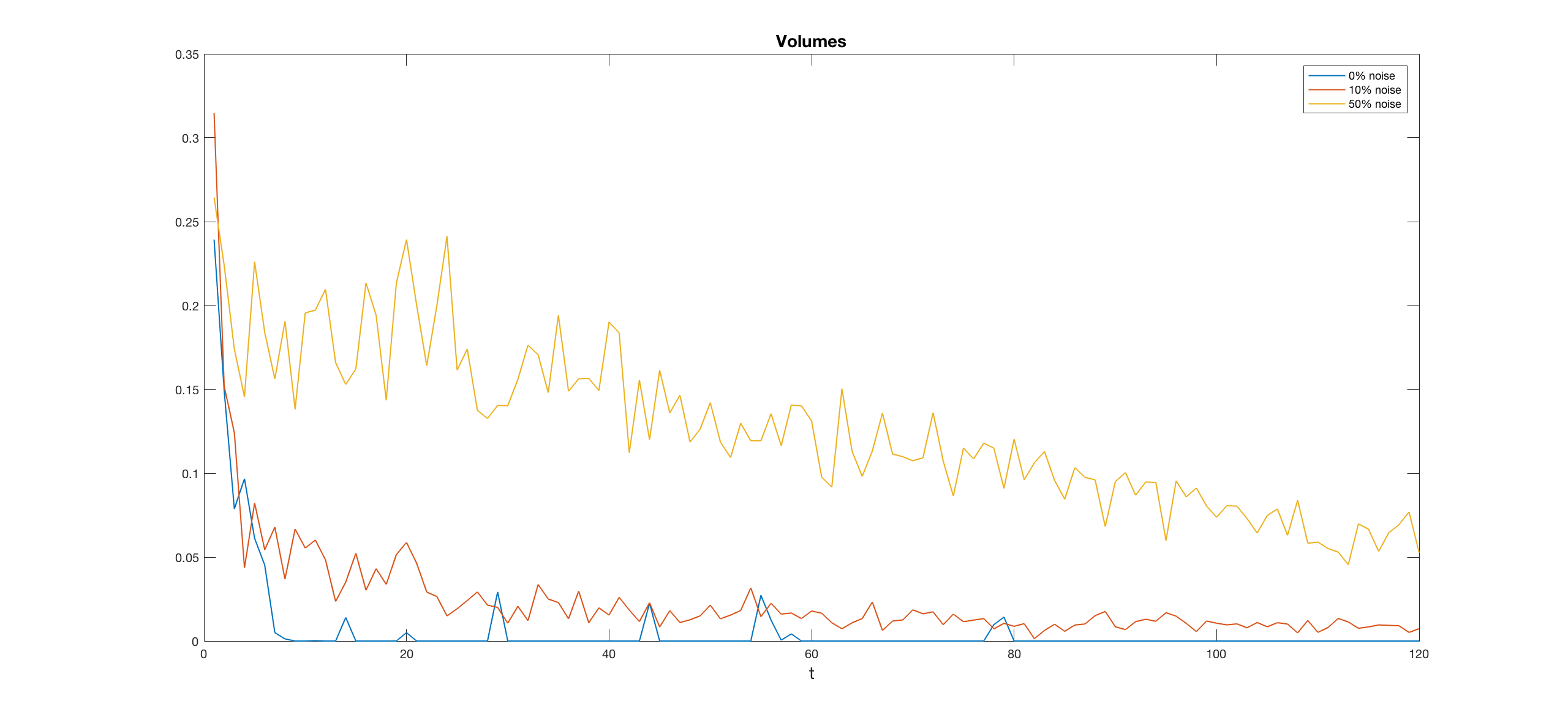
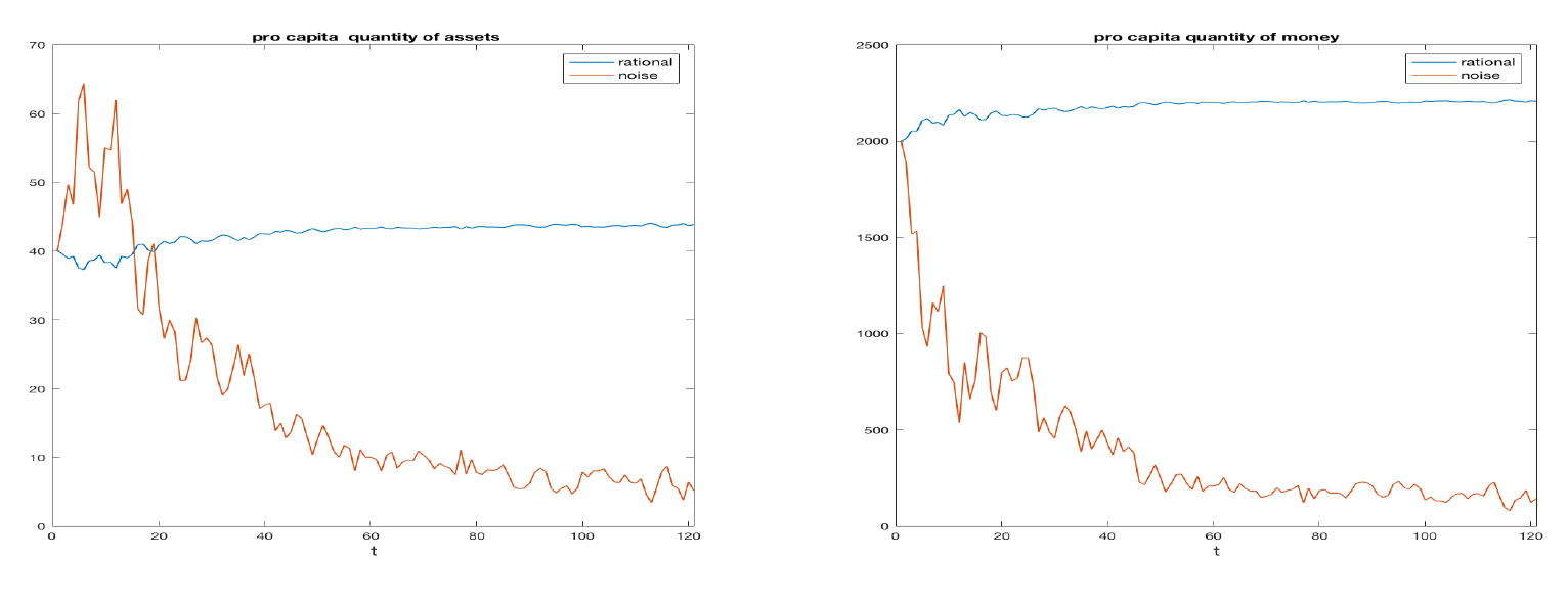
Figure 1 shows the average percentage volume exchanged across simulations as a function of time for three cases, corresponding to 50%, 10% and 0% of the traders being noise ones. In this experiment, we kept the number of convex contracts equal to 50% of the total. We performed 1000 simulations, with T = 100 and N_agents = 100. For each of the three cases, we see that volumes decrease with time, indicating that after a certain point, agents almost stop their trading. In general, and not surprisingly, noise traders increase the volumes of exchanges. To study the distribution of wealth between noise traders and rational ones we report in Figure 2 the average units of assets (left) and the average amount of cash (right) per capita as a function of the time, for the case of 10% of the traders being noise ones. We note the transfer of wealth from the noise traders to the rational ones. This is in line with Sandroni (2000) who studied the conditions for the extinction of noise traders in a competitive market.

**Figure 1**. Volumes are reported for three percentage of noise agents, 0%, 10% and 50%. As expected, volumes increase as noise agents percentage increase. In this plot, the percentage of convex contract is 50.

**Figure 2**. Average wealth per capita of noise and rational traders as a function of time. The left plot represents the units of asset, the right one the cash. Noise traders are 10% of the total. Contracts are half linear half convex.

Correlation between risk aversion and wealth

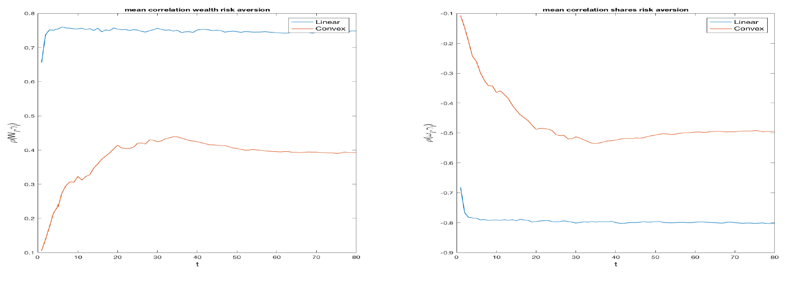
To study how the specification of the contract affects the decisions of the rational traders, we computed, for each simulation and for each time t, the correlations between the risk aversions and the cash or the units of assets hold by each rational agent. We represent the mean values across the simulations of the two correlation for each t in Figure 3 for the cases of all linear contracts and all convex contracts. For both contracts, the mean correlation is always positive for the cash (left) and negative for the units of asset (right). This is expected, since higher risk aversion should lead to a position with more cash and less assets. We also see that convex contracts exhibit a lower correlation (in absolute value), which is sometimes not even significantly different from zero. This means that convex incentives strongly affects the choices of the traders, by weakening the influence of their risk aversions. We note that the correlation starts from zero, since the initial endowments are constant among agents and then it converges towards a constant level. In the linear case, the stable level is reached earlier.

**Figure 3**. Correlation at each time t between risk aversion and cash (left hand side) or units of asset (right hand side).

Market Prices and Equilibrium Prices

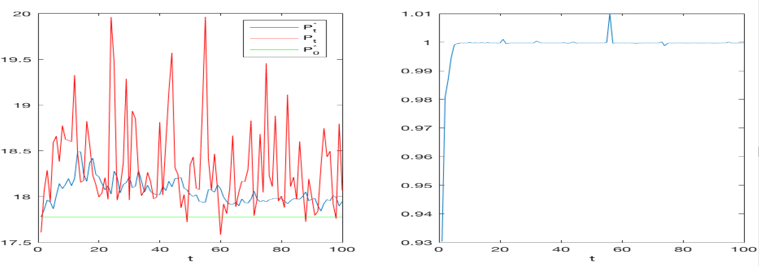
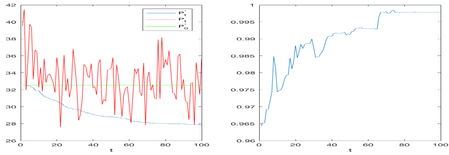
To evaluate the efficiency of the double auction market and the influence of linear and convex contracts, we observe the market prices $P_t$ and compute the equilibrium prices $P^*_t$ and the corresponding total equilibrium utility $U^*_t$ as well as the total utility $U_t$. In a first set of 1000 simulations, we considered 90 rational traders endowed with a linear contract and 10 noise traders. In the second set, the rational traders had a convex contract. Figures 4 and 5 refer, respectively, to the linear and to the convex cases. Each figure reports, on the left, the average market price $P_t$ across all simulations, the equilibrium price $P^*_t$ and a constant line representing the equilibrium price at time 0, on the right, the average across all the simulations of the ratio between $U_t$ and $U^*_t$. Observing the figures on the left, we see that the prices for the linear case are much lower than those of the convex one. This is because the convex contract increases the demand for the risky asset, boosting its price. In the linear case, the market prices bounce around the equilibrium price. In the convex case, they tend to be above it and have wider oscillations. This fact may be a consequence of the characteristics of the demand functions, continuous for the linear contracts and discontinuous for the convex ones, see Figure 10 in Appendix A. Holders of the convex contract tend to assume more extreme positions, proposing and accepting exchanges at prices higher than equilibrium. The Figures on the right show that in both the cases, the ratio of the two expected utilities converge to one, meaning that the market mechanism is efficient and reaches a global welfare. However, we note that the convergence is faster in the linear case. As already observed in the previous analysis of the correlations (Figure 3), the presence of convex contracts make the market more unstable and slower in reaching a steady state.

**Figure 4**. On the left hand side, the market price is plotted with the static equilibrium and the dynamic equilibrium for T = 100, *N_agents* = 100, all linear contracts, 10% of noise traders. On the right hand side, the ratio between the total expected utility and the total equilibrium utility. Values approaching 1 means that the market is allocative efficient.

**Figure 5**. On the left hand side, the market price is plotted with the static equilibrium and the dynamic equilibrium for T = 100, *N_agents* = 100, all convex contracts, 10% of noise traders. On the right hand side, the ratio between the total expected utility and the total equilibrium utility. Contrary to the linear case, values approach 1 only on the long run.

The order book analysis

To analyze the order book quantities and their dependence on convex contracts, we simulated a market with 100 traders, varying the proportion of convex contracts between 0 and 1, while keeping noise traders percentage equal to 10%. Parameters are as given in Table 1. For any percentage of convex contracts we made 30 simulations and for each simulation we recorded the following quantities:

LOs: the total number of limit orders;
MOs: the total number of market orders;
MOBs: the total number of market orders from the buy side;
MOSs: the total number of market orders from the sell side;
LOBs: the total number of buy limit orders;
LOSs: the total number of sell limit orders;
LOBEs: the total number of executed buy limit orders;
LOSEs: the total number of executed sell limit orders.

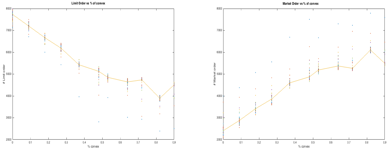
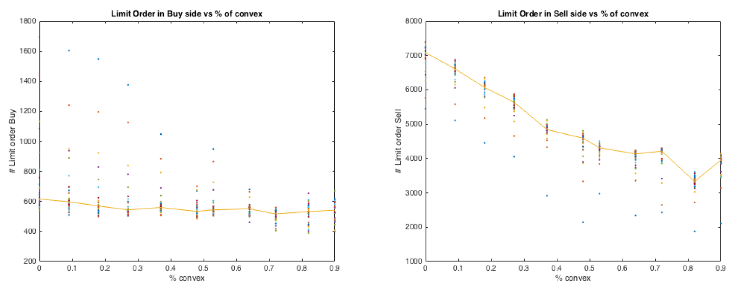
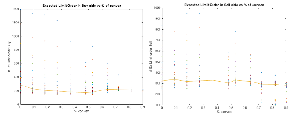
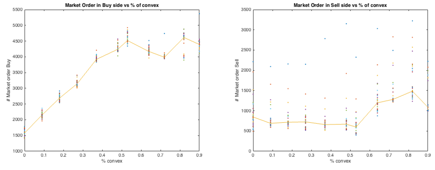
The main effect of a convex incentive is increasing the greed of the traders. This is evident when examining the number of limit and market orders versus the proportion of convex contracts. Indeed, Figure 6 shows that the number of limit orders decreases with the number of convex contracts, while market orders increase with it. Overall, the total amount of limit and market orders is independent of the percentage of convex contracts. Agents with convex contracts are more impatient and prefer submitting market orders rather than posting limit orders. Figure 7 shows how limit orders are distributed between bid and offer. We see that only the number of limit orders on the sell side reacts to the increase of convex contracts, while the number of those on the buy side remains constant. However, when we observe the number of executed limit orders, see Figure 8, we see that changing the ratio of convex contracts has no impact, both on the buy and on the sell side. This means that one of the effects of convex contracts is that of decreasing the number of the non-executed selling orders, as the traders submit offers at prices that are in general too high. Interestingly, we see that market orders exhibit an opposite behavior. In fact, see Figure 9, the number of market orders on the buy side increases with the percentage of convex contracts, while the number of market orders on the sell side stays almost constant. Agents endowed with convex contract tend to buy more than sell. We can observe that when the percentage of convex contract is above 50%, market orders on the sell side react weakly, while market order on the buy side become flatter. This can be a side effect because when more agents have similar demand functions, fewer exchanges take place. Such effect may also be visible in the right panel of Figure 7, where the number of sell limit orders decreases at a lower rate as the percentage of convex contracts approaches 100%. In conclusion, the order book analysis confirms that convex contracts do change the way agents post their orders as shown by the analysis in Appendix A. In particular, Figure 10 shows that a convex contract pushes a risk averse trader towards a demand similar to that of a more risk loving agent: convex contracts reduce risk aversion!

**Figure 6**. The number of limit orders (left panel) and the number of market orders (right panel) for 30 simulations plotted versus the percentage of convex contracts. The solid line is the median.

**Figure 7**. The number of buy (left panel) and sell (right panel) limit orders in 30 simulations versus the percent-age of convex contracts. The solid line is the median.

**Figure 8**. The number of executed buy limit orders (left panel) and executed sell limit orders (right panel) in 30 simulations versus the percentage of convex contract. The solid line is the median.

**Figure 9**. The number of buy market orders (left panel) and sell market orders (right panel) in 30 simulations versus the percentage of convex contract.

Conclusions

With our agent based model, we investigated the impact of convex contracts on the price dynamics and on the order book. We found that convex contracts produce higher prices and larger deviation of prices from the rational equilibrium (the price that clears the market when only rational traders are involved). However, we showed that our artificial double auction market is efficient as it permits convergence to a global welfare but the presence of convex contracts make such a convergence slower. Furthermore, our analysis on correlation shows that convex contracts have a strong influence on the decisions of the traders, dominating the effect of risk aversion.

The structure of the order book is strongly affected by the presence of convex contracts; in fact, they reduce the number of limit orders submitted on the sell side, while increasing the number of market orders from the buy side. Convex contracts encourage traders to buy more aggressively, increasing the total demand and consequently the market prices. The analysis of the order book shows that prices increase in presence of convex contract because convex contract pushes agents to buy more and to sell less, and to buy in a rush, using market orders rather than limit orders.

In conclusion, we remark that our model examined the effects of one particular kind of convex compensation, which is the option-like structure, which flattens bad outcomes, and linearly rewards good ones. This is the structure that is mostly used for real markets. We believe that our qualitative results still hold for the case of other convex structures, but this should be verified with further tests. Another important limitation of the present analysis is the assumption of myopic agents who optimize their portfolio as if there were only one period to go. By introducing expectations on the evolution of market prices and on the probability of a limit order to be executed, one could try to model a more complex and maybe more realistic model, where the agent perform a dynamic optimization and are not myopic but far-sighted.

Acknowledgements

A previous version of this paper was presented at the 11th edition of the Artificial Economics Conference, held in Porto on 3-4 September 2015. We would like to thank Tim Verwaart and Pedro Campos for editing the special section for JASSS and an anonymous referee for many helpful comments. This research was supported by the Swedish Research Council (grant 2015-01713).

Appendix

Appendix A: Rational demands

In this section, we analyze the optimization problem of the rational agent to give some insights on the optimal demand function and how it changes according to the contract type. Then we study the equilibrium price aggregating the agents’ optimal demand. Recall that the rational trader solves the problem (3). We consider separately linear and convex contract functions, starting from the linear case.

Let $\nu(\theta,P)$ be the first derivative with respect to $\theta$ of the expected utility of the final wealth $W(\theta,P)$, that is

$$\nu(\theta,P)=\frac{\partial}{\partial \theta}E [u(W(\theta,P))].$$

For any given price $P$, the function $\nu(\theta,P)$ is decreasing with respect to $\theta$ when the utility function is concave (risk-averse agent) while it is increasing for a convex utility. In the risk-averse case, the optimal demand $\theta^*$, that is the solution to problem (3), either satisfies the First Order Condition (FOC)

$$\nu(\theta,P)=0,$$

when it belongs to the feasible interval $[-\omega , \frac{C_0}{P} ]$. More precisely, it is equal to the lower bound $-\omega$ when the marginal expected utility $\nu(-\omega,P)$ is negative, it is equal to the upper bound $\frac{C_0}{P}$ when $\nu(\frac{C_0}{P} ,P)$ is positive, for all the remaining cases it lies within the feasible interval.

Thus, the optimal demand is the continuous function

$$\theta^*(P)=\left\{\begin{array}{ccc} \frac{C_0}{P} & \text{if} & P \le P^d\\ z(P) & \text{if} & P \in(P^d,P^u) \\ -\omega & \text{if} & P \ge P^u\\ \end{array}\right.$$

(7)

where $z(P)$ satisfies the FOC

$$\nu(z(P),P)=0,$$

$P^d$ is the solution to

$$\nu(-\omega ,P)=0.$$

When the agent is not risk averse, that is when his utility is a convex function, his optimal demand is

$$\theta^*(P)=\left\{\begin{array}{ccc} \frac{C_0}{P} & \text{if} & P \le P_{s} \\ -\omega & \text{if} & P \ge P_{s}\\ \end{array}\right.$$

(8)

where the switching price $P_{s}$ satisfies

$$E \left[u \left(W\left(\frac{C_0}{P},P\right)\right)\right]=Eu\left[ \left(W(-\omega,P) \right)\right].$$

(9)

Consider our case with a linear contract and a Constant Relative Risk Aversion (CRRA) we have

$$\nu(\theta,P)=E[(W_0+(\omega+\theta)X-\theta P)^{-\gamma} (X-P)].$$

In the risk-averse case, that is for $\gamma$ positive, it is easy to obtain $P^u=E[X]$ and

$$P^d=\frac{E[X^{1-\gamma}]} {E[X^{-\gamma}]}.$$

The demand function is

$$\theta^*(P)=\left\{\begin{array}{ccc} \frac{C_0}{P} & \text{if} & P \le \frac{E[X^{1-\gamma}]} {E[X^{-\gamma}]}\\ z(P) & \text{if} & P \in(\frac{E[X^{1-\gamma}]} {E[X^{-\gamma}]},E[X]) \\ -\omega & \text{if} & P \ge E[X]\\ \end{array}\right.$$

(9)

When the agent is risk-neutral, i.e. when $\gamma=0$, we get

$$P^u=P^d=E[X]$$

and the optimal demand function becomes

$$\theta^*=\left\{\begin{array}{ccc} \frac{W_0}{P} & \text{if} & P < E[X] \\ -\omega & \text{if} & P > E[X] \\ \end{array}\right.$$

Note that in the case $P=E[X]$, the agent is indifferent between buying or selling any amount of the asset and Problem is solved by any feasible $\theta$.

When the contract function is convex and the agent is risk-averse, the expected utility in Problem (3) is piece-wise concave as a function of $\theta$. The reason of the piece-wise concavity stems from the fact the contract function in this case is piece-wise linear. Since the asset $X$ assumes only two values, the expected utility has two nodes, corresponding to the values of $\theta$ satisfying

$$W_0+(\omega+\theta )X_i-\theta P= K, \quad i=1,2$$

In this case, the optimal demand $\theta^*(P)$ may coincide with the boundaries of the feasibility interval. This leads to an optimal demand function always discontinuous, which can be found only numerically. It is defined as in equation (8) for any value of the parameter gamma.

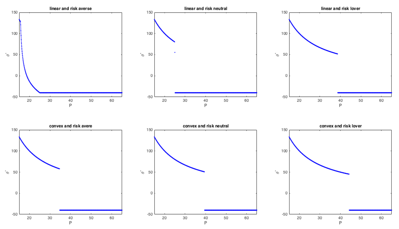
Figure 10 represents the optimal demand functions in all cases, linear contract first line and convex contract second line for different levels of risk preference. The demand function is continuous for a risk-averse agent, but it is discontinuous for a risk-neutral and a risk-seeking agent. The discontinuity point is the highest price $P_{s}$ at which the agent is willing to invest all the money in the risky asset. It can be identified by solving Equation (9). The value of $P_{s}$ depends on the risk preferences and it decreases with the level of risk preference $\gamma$. When the incentive is convex, the optimal demand function is always discontinuous, independently of the risk preferences. By comparing the plots in the linear and convex case in Figure 10, we found that the convex incentive increased the demand of the risky asset for each level of risk propension.

**Figure 10**. On the left hand side, the market price is plotted with the static equilibrium and the dynamic equilibrium for T = 100, *N_agents* = 100, all convex contracts, 10% of noise traders. On the right hand side, the ratio between the total expected utility and the total equilibrium utility. Contrary to the linear case, values approach 1 only on the long run.

Appendix B: The equilibrium price

We can consider theoretical the equilibrium price only when all the traders are rational. The equilibrium price is the price which clears the market, that is the value $P$ that solves the Equation (4)

The aggregate demand function is a not increasing function of $P$, with a number of points of discontinuity that is less than or equal to the total number of agents. Given that the aggregate demand is discontinuous, Equation (4) may not have a solution, and hence an equilibrium price may not exist. However, we can always identify the value, where the aggregated demand changes its sign. This price, denoted by $P_{eq}$ represents the price that maximizes the volume of exchanges between the agents. We call it the "quasi-equilibrium" price. Of course, any equilibrium price is also a quasi-equilibrium price.

For the existence of an equilibrium price, there must be a sufficient degree of heterogeneity among agents. We assume that agents have the same initial endowment ($C_0$ units of cash and $\omega$ units of asset). Therefore, if they also have the same level of risk preference and the same contract function, they will make the same choices and obviously no price can clear the market (however, also in this case, there would exist a quasi-equilibrium price). When agents’ preferences or contracts exhibit enough variation among agents, the market clearing condition (4) could be satisfied.

To clarify this point, let us consider a simple example with only two agents whose demand functions are

$$\theta^*_i(P)=\left\{\begin{array}{ccc} \frac{W_0}{P} & \text{if} & P \le P_{si}\\ -\omega & \text{if} & P > P_{si} \end{array}\right.$$

with $P_{s1} \leq P_{s2}$. By aggregating the demands we get

$$\sum_{i=1}^2 \theta^*_i(P)=\left\{\begin{array}{ccc} 2\frac{C_0}{P} & \text{if} & P \leq P_{s1} \\ \frac{C_0}{P} -\omega & \text{if} & P_{s1} < P \leq P_{s2} \\ -2\omega & \text{if} & P > P_{s2} \\ \end{array}\right.$$

The aggregate demand is equal to zero only if $P_{s1} \neq P_{s2}$, that is when the two agents have different preferences. In such a case, the equilibrium price $P_{eq}$ exists and is equal to $\frac{C_0}{\omega}$ if and only if $P_{s1} < P_{eq} < P_{s2}$, thus it depends on the utility functions and on the type of the contract through the values $P_{si}$.

It is possible to generalize the previous argument to a set of $N$ agents with discontinuous demand functions given by

$$\sum_{i=1}^2 \theta^*_i(P)=\left\{\begin{array}{ccc} 2\frac{C_0}{P} & \text{if} & P \leq P_{s1} \\ \frac{C_0}{P} -\omega & \text{if} & P_{s1} > P \leq P_{s2} \\ -2\omega & \text{if} & P > P_{s2} \\ \end{array}\right.$$

$$\theta^*_i(P)= \frac{C_0}{P}{\bf 1}_{P>P_{si}} - \omega {\bf 1}_{P>P_{si}} \quad, i = 1, \dots, N$$

where ${\bf 1}_{A}$ is the indicator function of the set $A$. Assuming without loss of generality that the sequence of nodes $P_{si}$ is increasing, the equilibrium price exists and is given by

$$P_{eq} = \frac{N-\kappa}{\kappa} \frac{W_0}{\omega},$$

for an integer $\kappa$ between 1 and N-1, if and only if

$$P_{s\kappa} > P_{eq} > P_{s\kappa+1}.$$

Model Code

The model is publicly available in CoMSES Computational Model Library at this address: https://www.openabm.org/model/4984/version/1/view.

Notes

This setting is equivalent to consider two types of agent, an investor who invests her own wealth and a portfolio manager who invest money on behalf of others. Under this interpretation this model offers a tool to study the impact of intermediation on financial markets.
This rule was inserted to simplify the optimization problem faced by the trader, but it is also important to enhance the allocative efficiency of the market, see LiCalzi & Pellizzari (2008).
Here and in what follows, when not explicitly indicated we mean the uniform distribution.

References

ALLEN, F. & Gorton, G. (1993). Churning bubbles. Review of Economic Studies, 60, 813–836. [doi:10.2307/2298101]

BEBCHUK, L. & Spamann, H. (2010). Regulating bankers pay. Georgetown Law Journal, 98, 247–287.

BLUME, L. & Easley, D. (1992). Evolution and market behavior. Journal of Economic Theory, 58(1), 9–40. [doi:10.1016/0022-0531(92)90099-4]

DEWATRIPONT, M., Rochet, J. & Tirole, J. (2010). Balancing the Banks: Global Lessons from the Financial Crises. Princeton, NJ: Princeton University Press.

FABRETTI, A., Garling, T., Herzel, S. & Holmen, M. (2014). Convex incentives in financial markets: An agent-based analysis. Available at SSRN: http://ssrn.com/abstract=2529902.

FRENCH, K., Baily, M. N., Campell, J. Y., Cochrane, J. H., Diamond, D. W., Duffie, D., Kashyap, A. K., Mishkin, F. S., Rajan, R. G., Scharfstein, D. S., Shiller, R. J., Shin, H. S., Slaughter, M. J., Stein, J. C. & Stulz, R. M. (2010). The Squam Lake Report: Fixing the Financial System. Princeton, NJ: Princeton University Press.

GENNAIOLI, N., Shleifer, A. & Vishny, R. (2012). Neglected risks, financial innovation, and financial fragility. Journal of Financial Economics, 104, 452–468. [doi:10.1016/j.jfineco.2011.05.005]

GODE, D. & Sunder, S. (1993). Allocative efficiency of markets with zero-intelligence traders: Market as a partial substitute for individual rationality. Journal of Political Economy, 101, 119–137.

HOLMEN, M., Kirchler, M. & Kleinlercher, D. (2014). Do option-like incentives lead to overvaluation? Evidence from experimental asset markets. Journal of Economic Dynamics and Control, 40, 179–194. [doi:10.1016/j.jedc.2014.01.002]

LICALZI, M. & Pellizzari, P. (2008). Zero-intelligence trading without resampling. In Complexity and artificial markets, (pp. 3–14). Springer Berlin Heidelberg.

LONG, J. B. D., Shleifer, A., Summers, L. H. & Waldmann, R. J. (1990). Noise trader risk in financial markets. Journal of Political Economy, 98, 703–738. [doi:10.1086/261703]

MALAMUD, S. & Petrov, E. (2014). Portfolio delegation and market efficiency. Working Paper Swiss Finance Institute, EPF Lausanne.

RAJAN, R. G. (2006). Has financial development made the world riskier? European Financial Management, 12, 499–533 [doi:10.1111/j.1468-036X.2006.00330.x]

SANDRONI, A. (2000). Do markets favor agents able to make accurate predictions? Econometrica, 68(6), 1303–1341

SOTES-PALADINO, J. M. & Zapatero, F. (2014). Riding the bubble with convex incentives. Marshall Research Paper Series Working Paper FBE, 06. [doi:10.2139/ssrn.2471082]