Can Redistribution by Means of a Progressive Labor Income-Taxation Transfer System Increase Financial Stability?

Introduction

The recent financial crisis in the USA led to a major downturn of the world economy. With the benefit of hindsight, many factors have been identified as leading to the crisis. Amongst others the increase of income inequality was frequently mentioned by many popular commentators (see e.g. Rajan 2010 or Reich 2010). Their main rationale is that in the presence of low interest rate levels financial intermediaries started to expand the activities of house financing for the group of low-income households (the so-called subprime segment). This shift to risk was backed by government officials, opaque financial innovations for risk transfer, and special bankruptcy rules in the US allowing for only adhering with collateral and not with personal wealth. The increased collateral value of the house was also employed to lever up for other forms of consumption (rather than housing) and thereby allowing low-income individuals to keep up with the Joneses in terms of consumption. As the house prices collapsed many individuals were confronted with the need to massively delever resulting in the severe worldwide economic downturn.

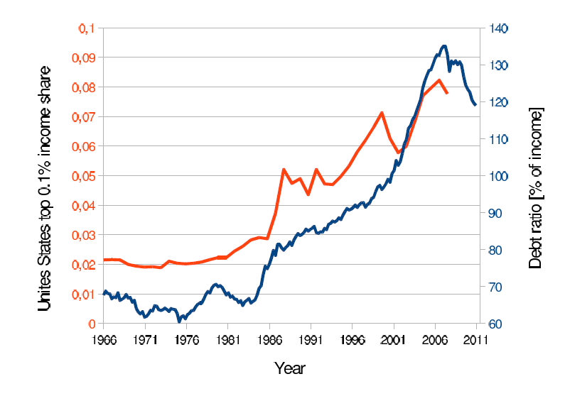
The empirical evidence for the USA suggests a relationship between private debt and inequality. Figure 1 presents the share of the top 0.1% - as a measure of inequality - and the share of private debt (household and non-profit organizations) to disposable personal income. There is a significant positive correlation between the two measures amounting to 0.95.

Theoretical models try to capture the underlying mechanism. It has been studied in some theoretical models using either Dynamic Stochastic General Equilibrium (DSGE) methodology (Kumhof et al. 2015) or the Agent-Based Model (ABM) approach (e.g. König and Größl 2014) or Cardaci (2014). The latter approach seems highly fruitful for the considered questions as this modeling in particular embraces heterogeneity and social interaction which are in the core of the underlying issue. Moreover, the issue of instability is not ruled out by assumption. The model considered in this paper was introduced in Fischer (2013). In this paper, numerical simulations suggested a positive relationship between inequality and financial stability. This paper recaptures the model and enhances the latter paper substantially by showing various robustness checks and in particular pointing to the underlying mechanism using closed-form solutions of (a slightly simplified) version of the model.

From the perspective of low-income individuals the gap between desired consumption level (the proverbial Joneses) and current labor income increases with inequality. Debt provides a short-term solution to the issue. The latter is willfully supplied by high income individuals making them build up high net-worth positions. The higher net worth increases speculation in financial markets, which can produce price bubbles in the model due to the complex interaction of chartist and fundamentalist rules. Higher prices also relax the collateral constraint and increase borrowing. Once the price bubble of risky assets burst, massive deleveraging sets in. Thus, the markets of risky assets and consumption goods are related in a non-trivial manner.

The second contribution of the paper comes from a policy perspective. Given the discussion about the financial crisis and the documented massive increase in inequality (e.g. Piketty 2014), there was a call for higher taxation (e.g. Diamond and Saez 2011). Given the above argument higher redistribution of labor-income - being the original source of inequality in the model - is expected also to enhance financial stability. Thus, it is expected that the research question asked in the title of the paper should be answered in an affirmative way. Yet, the paper provides a cautious note on this question. We discuss a self-financing labor income-taxation and transfer system. While the tax - by taking from the rich - reduces speculation on asset markets, it has some adverse welfare effects. In particular, the redistribution leads to an increase in the relative consumption level requiring a higher level of debt, leading to a potential increase in financial instability due to overborrowing of low-income individuals. Higher borrowing increases the rate of interest. The increased borrowing costs in turn lead to a higher borrowing implying the possibility of unstable Ponzi-Schemes. Moreover, we show that the lower level of income inequality (flow), is eventually accompanied by higher levels of net-worth inequality due to increased borrowing.

The remainder of this paper is organized as follows. Section 2 presents the baseline model and discusses the relationship between inequality and financial stability using both simulations and the underlying mechanisms. In Section 3 the modeling of the tax system is introduced and investigated by means of numerical simulations in Section 4. The final section wraps up.

Results in the Baseline Model

This section presents the basic underlying model also featured in Fischer (2013). The mechanisms leading to financial (in)stability are discussed in section about financial instability, using a simplified version of the model. Section 3.4 presents a simulation study discussing the role of inequality on financial stability in a calibrated version of the model. The robustness of the model results is checked in Section 3.17.

The Model

This section describes the underlying model. The code is available online. We discuss a dynamic model of \(i=1, \cdots, N\) heterogeneous households at periods \(t=1,\cdots, T\) that receive an exogenous labor income \(y_{i}\) that is unequally distributed. Households employ this labor income for consumption \(c_{i,t}\). Moreover, they buy a certain amount of risky assets \(d_{i,t}\).

The general timeline of the model is documented in Figure 2. Based on their current wage income \(y_{i}\), their current risky asset holdings at current prices \(q_{i,t}P_t\), and their indebtedness \(D_{i,t}\) households make their decisions about consumption which determine their (dis)savings. Some very low income agents might be forced to decrease their consumption. As soon as all \(N\) costumers have made their consumption/investment plans, markets for risky assets and savings decide new prices in order for markets to clear. At the end of every simulation period cumulated measures such as Gross Domestic Product (GDP) as well as distributional indices such as the Gini-coefficient of net worth are calculated.

The flow equation is given as follows:

$$ \Delta{D}_{i,t}=D_{i,t+1}-D_{i,t} = -\underbrace{(y_{i} - c_{i,t} - P_t d_{i,t})}_{\textrm{savings}} + r_t D_{i,t}. $$

(1)

If total income exceeds income, households are net savers and accumulate claims \(D_{i,t}<0\)). In the opposing case, households accumulate debt \(D_{i,t}>0\)). Initially, agents are endowed with zero debt \(D_{i,0}=0\)). The risky assets are traded at the current market price \(P_t\). The interest rate \(r_t\) for debt/claims increases with excess supply of savings. Any (temporary) imbalance in the savings market is assumed to represent a current account surplus (in the case of excess savings) or - in the opposing case - a current account deficit that is passively filled by foreigners. On an individual level net worth is computed as follows:

$$ W_{i,t}=P_t q_{i,t}-D_{i,t}, $$

(2)

where \(q_{i,t}=q_{i,t-1}+d_{i,t}\) represents the amount of risky assets which are activated at the current market price in the balance sheet. In fact, net worth is the current value of asset (being the wealth) net of debt.

The consumption is modeled following D’Orlando and Sanfilippo (2010), who present a Keynesian ad-hoc consumption function founded on behavioral theory:

$$ c_{i,t}= \bar{c}+ c_y \cdot max \{ 0;(y_{i}-r_t D_{i,t}) \} + c_w \cdot max \{0; W_{i,t}\}, $$

(3)

with different Marginal Propensities to Consume (MPCs) for different input factors \(0<c_w<c_y<1\)) and a subsistence level of consumption. One key assumption of our model is that the latter is derived from a relative consumption motive (Duesenberry 1949) and is computed as follows:

$$ \bar{c}=quantile_j(y_{i}). $$

(4)

The quantile \(j\) describes the minimum income that households want to consume. This level therefore crucially depends on the income distribution. In fact, this is a minimum consumption level uniform for all individuals. This can be considered the income level of the proverbial Joneses no family wants to fall short off with respect to consumption in order to indicate to their peers (Duesenberry 1949).

In a next step, households decide on how much to invest in risky assets. In our model, risky assets can be taken as collateral against which to borrow. To form the demand for risky assets, we closely follow the literature on Heterogeneous Agent Models (HAMs) in financial markets to model a market with endogenous boom/bust behavior. Households decide how many risky assets to buy based upon the result of a optimization with Constant Relative Risk Aversion (CRRA) of \(\varrho\):

$$ P_t q_{i,t}=\frac{E_t^k(p_{t+1}-p_{t})-r_{t}}{\varrho \sigma^2}\cdot W_{i,t} \; . $$

(5)

We use the nomenclature of upper case letters for real prices \(P_t\) and lower case letters for log-prices \(p_t\equiv\ln(P_t)\). The difference of log-prices in a first order approximation equals the expected return of the risky asset.

It is well-known that the share of risky assets decreases with the product of risk aversion \(\varrho\) and the volatility of the stock prices \(\sigma^2\). There are different formation mechanisms in order to form the level of price expectations \(E^k(p_t-p_{t-1})\). In our model, demand does not depend on wealth but on net worth \(W_{i,t}\) to control for the effect of debt. Agents decide to buy risky assets when they expect their prices to increase in the future, in time of low risk aversion \(\varrho\), and especially in times of low interest rates \(r_t\). The latter effect not only captures the effect that borrowing is cheap, but also that saving the money in other investment opportunities yields low returns.

There are two different paradigms for forming expectations - a stabilizing fundamental approach and a trend-following chartist approach. Fundamentalists expect prices to converge to their fundamentals and trade with an aggressiveness \(\beta_F>0\):

$$ E_t^F(p_{t+1}-p_{t})=\beta_F (f_t-p_t) \; . $$

(6)

We assume that the fundamental value is constant in time and normalize it to one \((F_t\equiv F \equiv 1\)) making the log-fundamental value zero \((f=\ln(F) \equiv 0\)).

Chartists on the other hand follow the recent trend with aggressiveness \(\beta_C>0\):

$$ E_t^C(p_{t+1}-p_{t})=\beta_C (p_t-p_{t-1}) \; . $$

(7)

As a result, the expectation of increasing prices can not only be due to a fundamental underpricing (as considered by fundamental traders), but also due to a self-fulfilling trend following strategy.

The weight of each strategy varies in time and is computed according to the Multinominal Logit Model giving the weight of a specific strategy \(k\) based on its attractiveness \(A_t^k\) (Manski et al. 1981):

$$ w_t^k=\frac{\exp(\gamma A_t^k)}{\sum_{i=1}^2 \exp(\gamma A_t^i)} \; . $$

(8)

The parameter \(\gamma\) can be interpreted as the degree of rationality, where for \(\gamma=0\) all strategies always have equal weight and for \(\gamma \rightarrow \infty\) agents always switch to the currently best strategy.

Following a very popular modeling strategy e.g. laid out in Hommes et al. (2009), the attractiveness of a trading strategy \(k\) \(A^k_t\) is computed as follows:

$$ A_t^k=\frac{E_t^k(p_{t+1}-p_{t})}{\sigma^2\varrho }(p_{t+1}-p_{t}-r_{t})+\lambda A_{t-1}^k \; $$

(9)

which - given the demand for assets in equation 5 - can be thought of as the return on investment. The latter is in particular high if agents are able to predict the market correctly and timely. The parameter \(0<\lambda<1\) can be thought of as the memory of the agents where low values reflect myopic trading.

Finally, there is always a certain degree of noise demand \(d_t^{noise} \sim N(0,\sigma^2_{noise})\) in the market. Noise trading results from idiosyncratic asset demand. A tangible example would be the case where a household becomes parents and has to sell some of their financial assets in order to cover for the respective expenses. Noise trading makes up a large chunk of overall financial market trading (Black 1986). The overall expected return is given by:

$$ E_t(p_{t+1}-p_{t})= w_t^CE_t^C(p_{t+1}-p_{t})+w_t^FE_t^F(p_{t+1}-p_{t})+d_t^{noise} \; . $$

(10)

In fact, it is a weighted average of the fundamental and chartist strategy (and noise trading).

It is important to point out that agents delegate their portfolio composition to some professional individuals (e.g. fund managers) who distribute portfolio share in risky and risk-free assets in a rational manner as laid out in Merton (1971), but follow some rules of thumb when forming expectations (eq. 7 and 6). Thus, despite \(N\) agents there are only \(n=2\) trading rules. The individual consumption follows the rule of thumb logic presented in eq. 3 and is individual.

The maximum level of debt is given by a collateral constraint allowing:

$$ D_{i,t} \leq D_{i,t}^{max}=(1-m) P_t q_{i,t}. $$

(11)

In this case \(m\) reflects the required equity ratio. More generally, this can even be thought of as the measure of financial development, for which low values represent highly evolved financial markets.

Agents can be classified into classes depending on the ability to consume. (i) Upper class agents are net savers, whereas the (ii) middle class and the (iii) lower class are net debtors. Agents can be ranked according to their labor income going from low to high. The net asset accumulation for high income households, as well as the net debt for low and middle income households, results from the combination of an exogenous subsistence level of consumption \(\bar{c}\) and MPCs smaller than one. We assume that the initial endowment of assets is perfectly correlated with the (non-time varying) labor income \(q_{i,0}=H y_i\) by means of a heritage \(H>1\). As a result, the lowest income agents face a binding collateral constraint, cannot borrow up and thereby fail to realize their consumption plans. In contrast to this, the middle class are indebted, but can, however, realize all their consumption plans, resulting in three different classes. Thus, the binding borrowing constraint is what distinguishes low class from middle class agents. In the model - and in line with empirical evidence (Doepke et al. 2006) - the middle class hold the highest amount of debt. This is because - in contrast to upper-class agents - they demand debt and - in contrast to lower-class agents - are not constrained in their ability to lever up.

The reaction of the agents classified as lower class when required to deleverage is important for the aggregate dynamics. Delevering is in particular prevalent in asset bust when the value of the collateral decreases. The level of deleveraging is given by:

$$ \Delta {D}_{i,t}=\Delta {D}_{i,t}^{max}=(1-m)P_t q_{i,t}-D_{i,t}<0. $$

(12)

Using equation 1 with the assumption that lower-class agents do not trade in asset markets (\(d_{i,t}=0\)), we assume the following consumption function:

$$ c_{i,t}=max \{\Delta {D}_{i,t}+y_{i}-r_t D_{i,t},0 \}, $$

(13)

implying that agents never end up with the unrealistic result of negative consumption. Moreover, these agents refrain from participating in the market for risky assets. This is in line with the empirical study of Shorrocks (1982) showing that the share of risky assets increases with wealth. More recent and similar evidence for the USA is reported in Saez et al. (2016). Note that we exclude the interesting case of fire sales, which present another important mechanism that can generate instability at the interaction of both markets.

Finally, we have to define market clearing. Following the well-established approach in ABMs (cp. e.g. Chiarella et al. 2006) we assume that prices are computed using a market-maker approach. The log-price is computed according to:

$$ p_{t+1}=p_t+ \frac{\mu}{N} \sum_{i=1}^N \frac{E_t(p_{t+1}-p_{t})-r_{t}}{\varrho \sigma^2} W_{i,t}=p_t+ \frac{E_t(p_{t+1}-p_{t})-r_{t}}{\varrho \sigma^2} \frac{\mu}{N} \sum_{i=1}^N W_{i,t}, $$

(14)

for which \(\mu\) represent the illiquidity of the market. In particular, high values of \(\mu\) can be considered as very illiquid markets, meaning that temporary market imbalances (either excess supply or demand) lead to strong price changes and thus also to high price volatility.

The clearing of the debt/savings market is made in a similar way:

$$ r_{t+1}=r_t \exp\left( \frac{\mu_r}{N} \sum_{i=1}^N \Delta{D}_{i,t}\right)=r_0 \exp \left( \frac{\mu_r}{N} D_t \right). $$

(15)

This implies a positive relationship between the excess supply of debt and the interest rate being its price. We assume that savings markets are more liquid than markets for risky assets \((\mu_r<\mu)\). The formulation with the exponential operator (respectively with the log-prices in the former case) guarantees positive values for interest rates (respectively prices).

In the following we discuss how financial (in)stability becomes manifest in the model.

Financial (In)Stability in the Model

As we have two markets - the market for credit/claims and the market for risky assets - financial stability has two forms. The stability condition for the market for risky asssets can be approximated by:

$$ \sigma^2{\varrho}>0.5 \mu \bar{W}_t\beta_C, $$

(16)

where instability increases in the presence of chartist trading \(\beta_C>0\)) for low risk aversion \(\varrho\), high volatility \(\sigma^2\) in the market for risky assets, illiquid markets (high \(\mu\)) and high mean net worth \(\bar{W}_t\). The latter increases if a high amount of upper-class agents exists who accumulate a large amount of claims. As a result high inequality accompanied by a large share of upper-class agents destabilizes the market for risky assets and thereby leads to financial instability.

On the other hand, a high amount of low income agents leads to the fact that the economy accumulates large amounts of debt, making the level of the interest rate increase, further requiring a higher amount of debt, possibly resulting in unstable Ponzi schemes and thereby presenting another form of financial instability. The Ponzi scheme can be hindered by high equity requirements \(m\) providing an upper cap for the level of debt (cf. eq. 11). Note, however, that the equity requirement also depends on endogenous variables - in particular the price level \(P_t\) of collateral. An asset price boom - that in this model can result from fundamental news, low interest rates, or a self-sustaining trend following trading strategy - can soften the collateral requirements. If this is followed by an asset price bust, many households end with too large a level of debt and are required to deleverage. In contrast to the first form of instability focusing on the upper part of the income distribution, the latter crucially depends on the low income households.

Thus, finally inequality and financial stability are interconnected in a non-trivial way, requiring numerical solutions to explain their concrete interplay.

Exemplary Simulations of the Model

For the simulations we assume that labor income follows a log-normal distribution:

$$ y_{i} \sim L(\mu, \sigma_y) = L(\log(\bar{y}), \sigma_y). $$

(17)

In a first-order approximation, the resulting Gini-coefficient of this particular distribution can be described as a function of \(\sigma_y\) only:

$$ Gini(y) \approx\frac{\sigma_y}{\sqrt{\pi}}\approx 0.564 \sigma_y. $$

(18)

Therefore this popular measure of inequality can be controlled by the single parameter \(\sigma_y\). Concretely we assume \(\sigma_y=1\) implying \(Gini(y)\approx 0.56\) broadly in line with empirical evidence for the USA (Wolff 2013).

Table 1: Benchmark simulation parameters and initial conditions

Category	Symbol	Description	Value
Distribution	\(y_0\)	Median labor income	5
	\(\sigma_y\)	Inequality of labor income	1
	\(H\)	Heritage	20
Durable market	\(\beta_F\)	Aggressiveness of fundamental traders	1
	\(\beta_C\)	Aggressiveness of chartist traders	1
	\(γ\)	Rationality	200
	\(λ\)	Memory	0.98
	\(\tilde{\rho}\)	Pseudo risk aversion	20
	\(\sigma^2_{noise}\)	Variance of noise trading	0.05
Consumption	\(j\)	Quantile of subsistence consumption	0.2
	\(c_y\)	Marginal propensity to consume out of income	0.5
	\(c_w\)	Marginal propensity to consume out of net worth	0.01
Collateral constraint	\(m\)	Equity requirement	0.2
Markets	\(\mu\)	Market illiquidity for durables	0.01
	\(\mu_r\)	Market illiquidity for durables	0.005
Initial conditions	\(r_0\)	Initial interest rate	0.02
	\(D_{i,0}\)	Initial debt for all agents	0
	\(P_0\)	Initial price level in durable market	\(1 \equiv F\)

Rather than performing an econometric calibration we decided to rely on a reasonable tuning of the model allowing it to generate realistic features. The model not only requires making assumptions about the value of parameters but is also sensitive to the assumed initial conditions. Our tuning heavily relies on the closed-form solutions. The simulation parameters and initial conditions are presented in Table 1. Figure 3 presents the simulations result regarding inequality for the case of \(N=1,000\) agents.

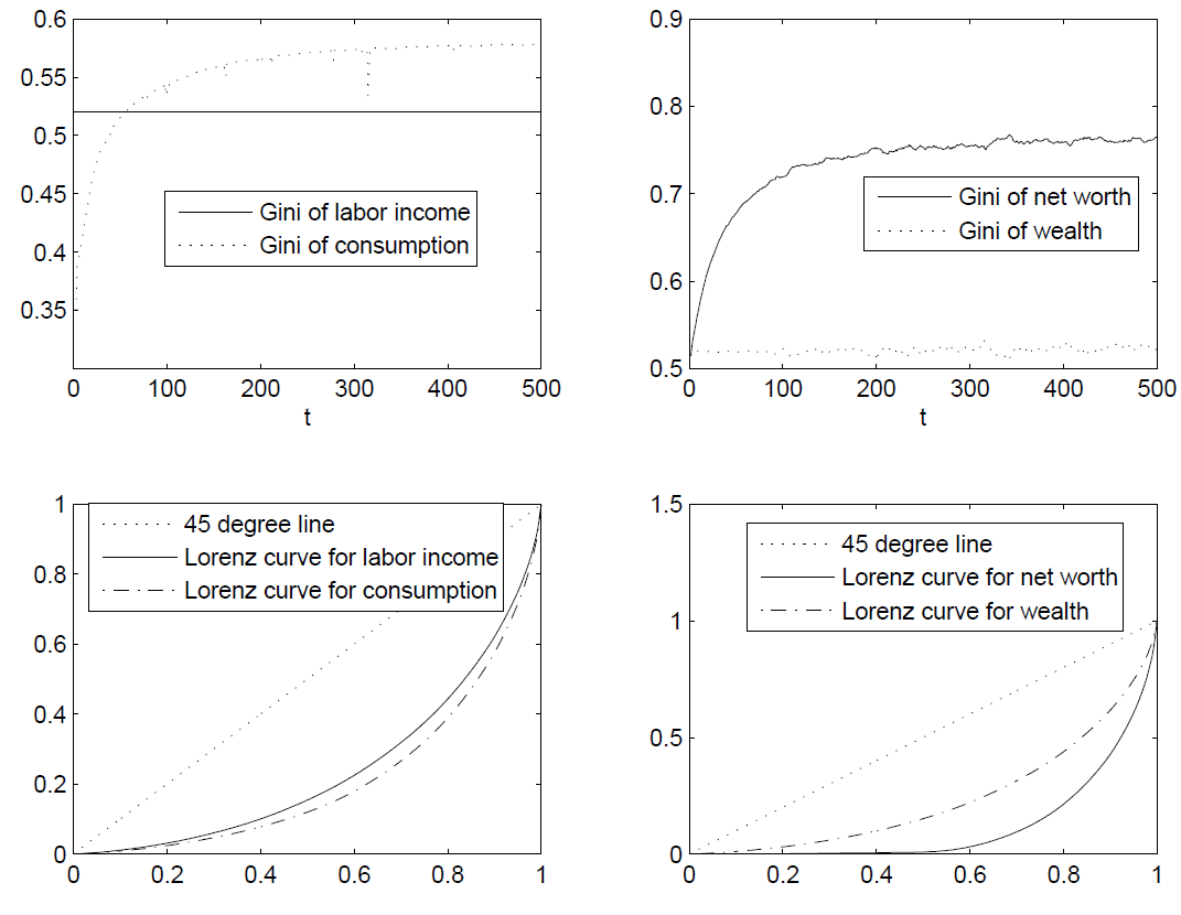
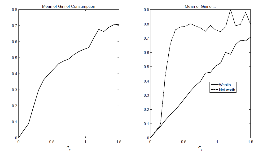
In our model the labor income as initial source of income inequality is constant in time (see Figure 3). Wealth inequality varies in time, yet the mean of income inequality and wealth inequality are identical. This can be linked to the fact that - in a CRRA world - portfolio structuring is independent of the level of wealth and our assumption that the initial distribution of wealth is directly related to the distribution of income.

Due to the initial condition of zero debt, the Gini of net worth starts at the identical level as wealth, but increases to a higher level due to the mutual accumulation of debt and claims. As suggested by empirical findings, the inequality of net worth (stock) is higher than the inequality in income (flow) (cp. e.g., Davies and Shorrocks 2000). In fact, in the recent crisis the Gini of net worth for the USA increased to a level of 0.87 (Wolff 2013), implying that our model even understates the true level of net worth inequality. The evolution of net worth inequality is an emergent behavior in the model propagated by debt. As net worth now, however, also affects consumption, this leads to the fact that consumption inequality in a dynamic process increases to a level above labor income inequality.

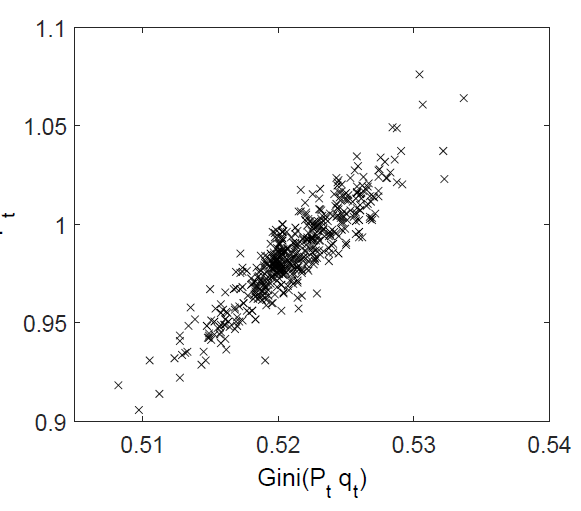
While the mean of wealth inequality is identical to income inequality, there is a positive correlation between the overall current price level and current wealth inequality as presented in Figure 4, implying that booms increase inequality of wealth. In a nutshell, the underlying rationale is that high-income individuals - not being in debt - have a higher equity ratio allowing for a stronger participation in booms. Low-income individuals face a binding collateral constraint which prevents them from levering up. It is only near the peak of the cycle, when prices are already high and the collateral constraint is very lax, that low-income individuals are able to go long in the asset market. However, by being amongst the last to jump the bandwagon they also suffer most from reevaluation losses in the subsequent bust. This is in line with the empirical evidence of Roine et al. (2009) showing that inequality increases in times of high asset prices and vice versa.

The model allows us to vary the degree of inequality - in a ceteris paribus manner - and discusses its impact by changing the value of the standard deviation of labor income \(\sigma_y\). In empirical discussions quantifying the effect of inequality is very difficult as it is interspersed with a variety of different factors that feed back in various directions. A natural experiment - satisfying the ceteris paribus assumption - is also hard to imagine in this domain, making the theoretic discussions still the most valuable tool for analyzing the effect of inequality.

It is important to note that we only have a finite sample of \(N=1,000\) agents. The draw from the distribution can vary severely. To control for this effect, we simulate each case multiple times and also aggregate along this dimension.

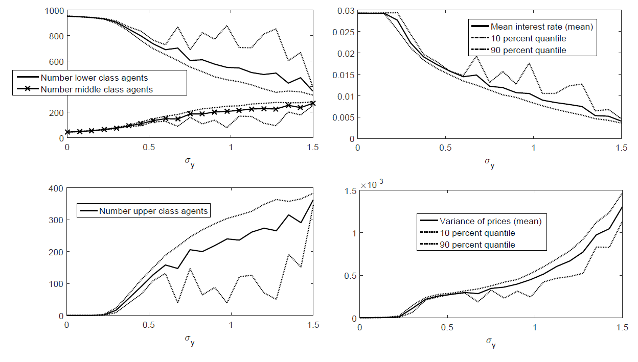
First of all, higher inequality changes the distribution of agents with respect to class (see Figure 5). More inequality leads to more upper-class agents.

Somewhat surprisingly, we have fewer lower-class agents and more middle-class agents. The latter factor can, however, be explained by the changing value of the relative consumption level. The rationale is that a higher inequality decreases the relative consumption level if \(j<0.5\) for a log-normal distribution. Since in our case we assume \(j=0.2\) this level decreases. Or put more bluntly, the reference level of consumption - the Joneses with whom all other agents try to keep up (Duesenberry 1949) - has a lower income in a more unequal society.

In effect, less debt is accumulated, interest rates decrease, but the volatility in markets for risky assets increases. The accumulation of capital available for speculative purposes due to a strong share of high-income individuals is the driving force behind this result. Note also that we find a direct negative relation between inequality and the equilibrium level of interest rates. The rationale is that the market for debt is mainly driven by supply, which increases with higher inequality.

The non-smooth behavior of the quantiles can be traced back to the presence of price bubbles - which is the (financial) instability in the model. As already discussed in the price boom, all agents lever up substantially decreasing the number of high class agents (cf. lower left panel of Figure 5). Meanwhile, the collateral constraint of low income relaxes making them also middle class (cf. upper left panel of Figure 5). The increased debt accumulation also manifests itself in the increased level of interest rate (cf. upper right panel of Figure 5).

We assume an exogenous increase in the inequality of labor income. As initial asset endowment is assumed to be perfectly correlated with the inequality of wealth, it equals the inequality of labor income. Other forms of inequality, however, grow at a different pace. As agents accumulate debt and claims net worth increase to a higher level (cf. Figure 6). This also feeds back to inequality of consumption which increases stronger than the income inequality. We can rank different economic figures according to their inequality:

$$ Gini(W)>Gini(C)>Gini(Y)=Gini(Pq), $$

(19)

with net worth being the most unequal measurement and the (exogenously assumed) factor of wealth and labor income are most equally distributed.

Robustness Check

The parameters associated with the risky asset trading are well tested in the literature of concerning the fundamental-chartist model (for an overview e.g. refer to Lux 2009; Chiarella et al. 2009; Hommes et al. 2009). Thus, the key novel parameters in our study are the ones related to consumption (i.e. \(j\), \(c_y\), and \(c_w\)). Essentially, all latter parameters increase the desire to consume and thus reshuffle a lot of agents to a lower class for a given income. Exemplarily, we show the simulation results for a variation of \(c_y\) here, while keeping all other parameters fixed as reported in Table 1. The higher demand for debt in order to increase consumption has the effect of increasing the interest rate on debt (cf. Figure 7).

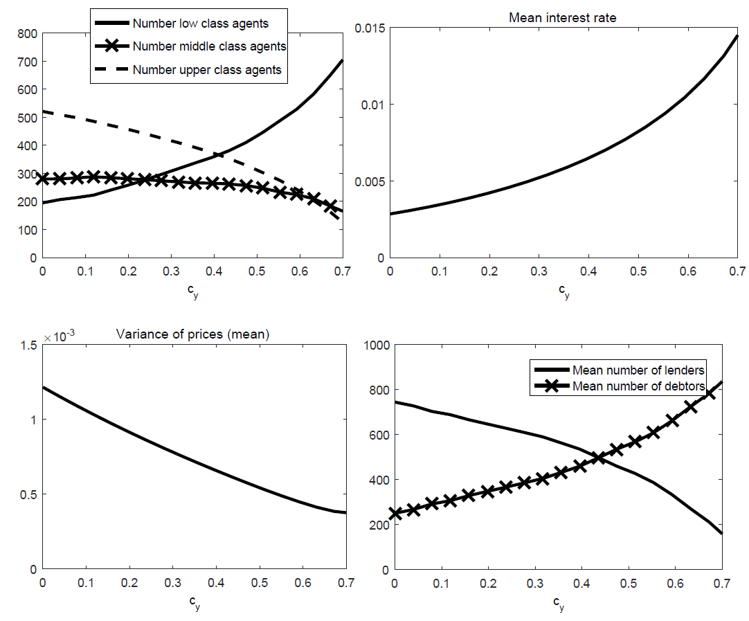
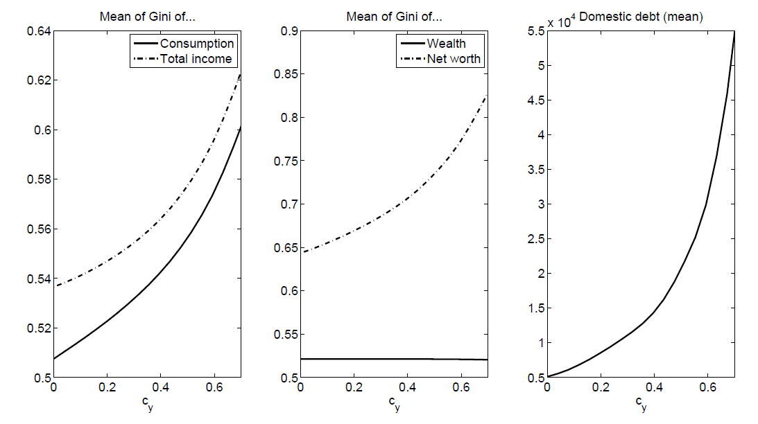
Meanwhile, the increased consumption decreases trading in the risky asset and thus also decreases volatility of asset prices (cf. the lower panel of Figure 7). As these agents employ debt in order to finance this consumption the net worth inequality increases (cf. Figure 8). The same holds true for the inequality of total income (\(y_{i}-r_tD_t\)) which also depends on debt. Essentially, changing the parameter changes the magnitude results of the model, while maintaining the overall mechanisms as stretched out in the previous discussion.

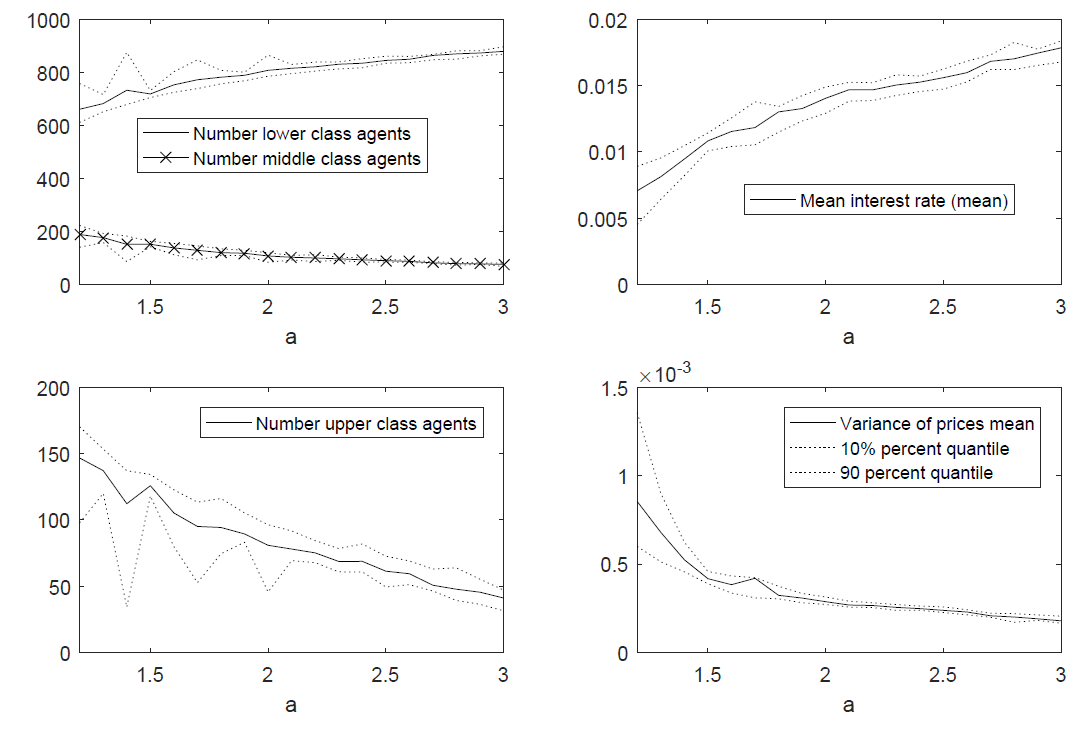
As a further robustness check, we also vary the concrete distribution. It is well-known since the investigations of Pareto (1896) that the upper tail of the income distribution is not well described by the log-normal distribution which we employed so far. The latter is well-described by a Power-law (or Pareto-distribution) with a cumulative probability density function:

$$ F(y)=1- \left(\frac{\tilde{y}}{y}\right)^{a}, $$

(20)

for \(a>1\). We set the mode of the Pareto-distribution \(\tilde{y}\) such that the mean for both distribution remain identical in order to have similar scales and vary \(a\). It is well-known that the Gini-coefficient is given by:

$$ Gini(y)=\frac{1}{2a-1}, $$

(21)

thus decreasing with \(a\). A reasonable value for the tail-coefficient is \(a=1.5\) implying a income share of the top 10% (top 0.1%; cf. Figure 1 ) of 46.4% (10%) and a Gini of 0.5.

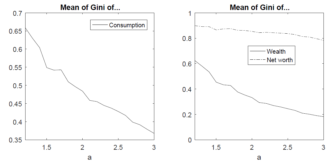
We vary the value of \(1.2<a<3\) and report the results in Figure 9. Qualitatively, the results are identical to the case with a log-normal distribution. Higher inequality - i.e. lower values of \(a\) - are accompanied by more upper class agents and (slightly) more middle class agents, making all individuals better off class-wise. The higher saving by the top income holders pushes down the interest rates and the volatility in financial market increases. Note that the measure is highly sensitive around the values of \(1.2<a<1.5\) for which the inequality (as measured by the Gini-coefficient) severely increases from approx. 0.5 to 0.7. As before, higher income inequality (modeled by lower values of \(a\)) also increases inequality of consumption, wealth, and net worth (cf. Figure 10).

Redistribution in the Model Economy

The model can account for several stylized facts of real economies. Moreover - and as already set forth in an earlier publication (Fischer 2013) - the model generates a positive relationship between inequality and financial instability. A natural solution to the problem therefore would be to introduce a taxation and transfer system that redistributes between agents, not only to combat inequality but also financial instability. Section 4.2 presents our modeling of a simple linear redistributive tax system and discusses it based upon numerical simulations in Section 4.10.

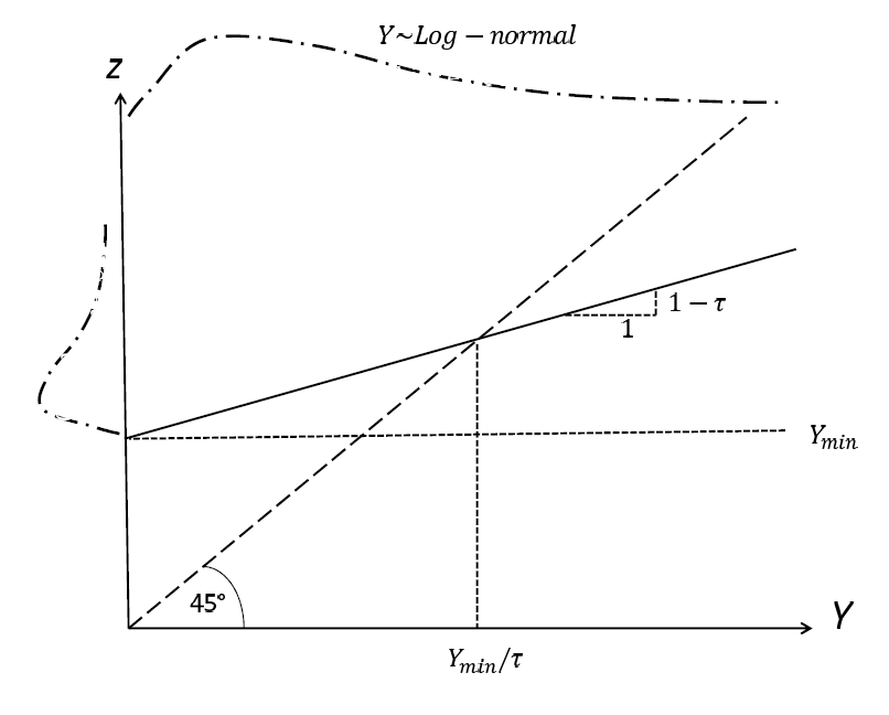
We assume that taxes are only imposed on labor income which we assume to be the exogenous source of income inequality. All individuals are subject to a flat income tax with a tax rate \(\tau\), while also receiving a basic income \(y_{min}\). The individual income after taxes \(z_i\) is thus given by:

$$ z_i=(1-\tau) y_i+y_{min}. $$

(22)

A different reading is that of a tax-free level \(y_{TF}\) that is exempt of taxation:

$$ z_i=(1-\tau)(y_i-y_{TF})+y_{TF}. $$

(23)

Comparing the two equations it is clear that \(y_{TF}=\frac{y_{min}}{\tau}\). Thus, the minimum income is always lower than the tax free income. The relationship between market income \(y_i\) and income after taxes and transfers \(z_i\) is depicted in Figure 11. This combined (linear) system of taxes and transfers is close to the negative income tax as proposed by Friedman (1962). In the public economics literature, the level \(y_{min}\) is also referred to as the demogrant, this being a minimum income level that is guaranteed to all individuals regardless of their respective labor income.

We want to assume a Robin Hood-tax whose only aim is to redistribute between individuals. The self-financing of the system requires:

$$ 0 \stackrel{!}{=} \sum_{i=1}^N (\tau y_i-y_{min})= \tau N \bar{y}- N y_{min}=N (\tau \bar{y}-y_{min}) \rightarrow \tau= \frac{y_{min}}{ \bar{y}}. $$

(24)

In this case, \(\bar{y}=\sum_{i=1}^N\frac{y_i}{N}\) is the mean income. The financing condition links the tax rate \(\tau\) and the minimum income \(y_{min}\) and thus only leaves one degree of freedom for shaping the tax system.

Table 2: Redistribution in various countries (Data source: OECD 2012)

Country	Redist
Mexico	0.02
USA	0.11
Canda	0.13
Japan	0.15
Spain	0.16
Sweden	0.22
France	0.22
Germany	0.23
Finland	0.25

A measure for the relative degree of redistribution \(Redist\) is the log-difference between the Gini-coefficient before (\(GBT\)) and after taxes and transfers (\(GAT\)):

$$ Redist=\log(GBT)-\log(GAT)=\log\left(\frac{GBT}{GAT}\right). $$

(25)

Table 2 presents some empirical evidence for the ratio.

This ratio is easy to transfer to our model. As shown in equation 18 (in a first-order approximation) for a log-normal distribution the Gini-coefficient is proportional to the standard deviation \(Gini(y) \sim \sigma_y\)). Due to the linearity property we have \(\sigma_z=(1-\tau) \sigma_y\). As a result:

$$ \log \left( \frac{GBT}{GAT}\right) \approx \log \left(\frac{\sigma_y}{(1-\tau) \sigma_y} \right)=\log \left( \frac{1}{1-\tau} \right) \approx \tau, $$

(26)

making the tax-rate \(\tau\) a simple index of redistribution. Given the empirical evidence presented in Table 1 values ranging up to \(\tau=0.35\) are empirically meaningful and chosen for testing the model in the following.

Effect of Taxation

In this section we present simulation results for the case with a tax on labor income \(y\). In this section, we take the benchmark model and vary the parameter \(\tau\) in a ceteris paribus fashion for reasonable levels of \(0<\tau<0.35\) as presented in Table 2. For this section, we assume that - rather than being formed on the distribution of the market income \(y_i\) - the subsistence level of consumption depends on the distribution of the post-tax income \(z_{i,t}\):

$$ \bar{c}=quantile_j(z_{i,t}). $$

(27)

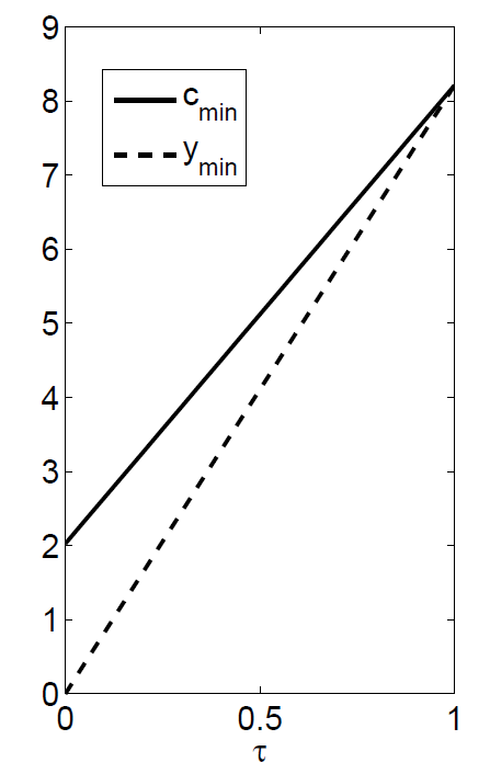
This assumption is essential for the results. As the post-tax income determines the available income for all agents, it is also the underlying variable for deriving the subsistence level of consumption. As shown in Figure 12, an increase in the tax level \(\tau\) increases the income level of the low-income households, also leading to a higher subsistence level of consumption. This is one of the central problems in redistributing flow income in the presence of relative consumption. The relative position of individuals does not change, while the minimum consumption level even increases. In fact, as also shown in Figure 12, the minimum consumption level is always above the minimum income provided by the tax system. Even though the gap between minimum income and minimum consumption narrows, it still persists (only converging to zero for an egalitarian society with \(\tau=1\)), requiring debt financing of consumption for some individuals.

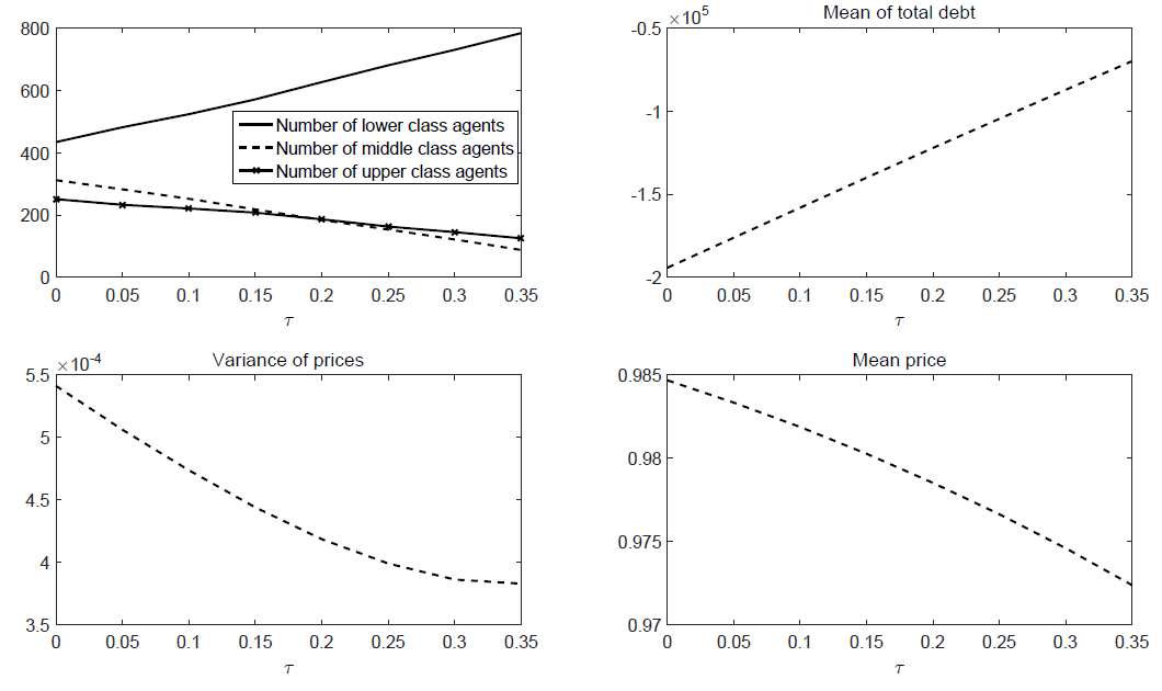
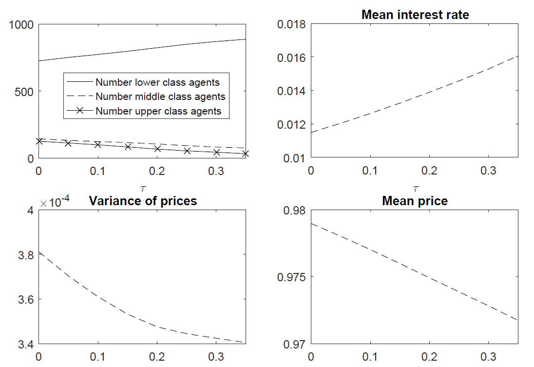
As shown in Figure 13, the Robin Hood-tax reduces the number of high-income households by taking from the rich. The social function of high-income households in the model context is to provide debt for lower income households. As the upper-class households vanish, the net-supply of debt decreases, accompanied by high interest rates. The high interest rate furthermore lowers the disposable income of lower income households, leading to an actual increase in lower-class households. Therefore, and somehow surprisingly, in a society with relative consumption, an income tax not only transforms upper-class into middle-class households, but also leads to the fact that middle-class households turn into lower-class households. As a result, the situation with taxes class-wise is Pareto inferior to a situation without taxes.

As presented in Figure 13, taxes reduce price volatility for risky assets and decrease their overall prices. This is because the share of upper-class agents participating in speculation in markets for risky assets decreases.

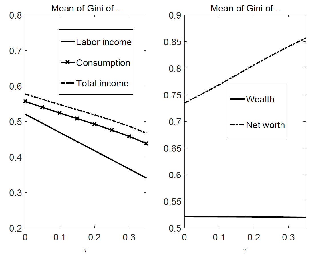
Finally, we can make a statement about different forms of inequality in the tax-regime case (see Figure 14). As already stated, the flat tax rate and labor income inequality can be related in a simple linear manner. Inequality of consumption, however, is above labor income inequality. In this region, the gap between these two forms of inequality increases due to consumption out of net worth (stock) as well as the total income inequality stemming from capital income. This effect can be attributed to the higher net worth (stock) inequality (documented in the right panel of Figure 14). Thus, the inequality of total income (i.e. capital and labor income \(x_i=y_i-rD_i\)) also decreases less than the inequality of (pure) labor income. While the tax is able to address the effects of flow inequality, the resulting increase in mutual debt/credit positions eventually increases the stock value of net worth inequality.

It is interesting to compare the approach with taxation - as presented in Section 3.4 - to the approach with an exogenous variation of inequality as presented in section "Exemplary Simulations of the Model". In this case as well, all agents are worse off in terms of class. Yet, for the exogenous variation we not only lower the level of income inequality, but also the level of wealth inequality, which we assume to be perfectly correlated (cf. Figure 6). The higher inequality of debt - due to a higher conspicuous consumption level in more egalitarian societies - is quantitatively less important than the lower inequality of wealth. As a result the distribution of net worth is more egalitarian for the case of an exogenous decrease in inequality in contrast to the case with higher labor taxes \(\tau\).

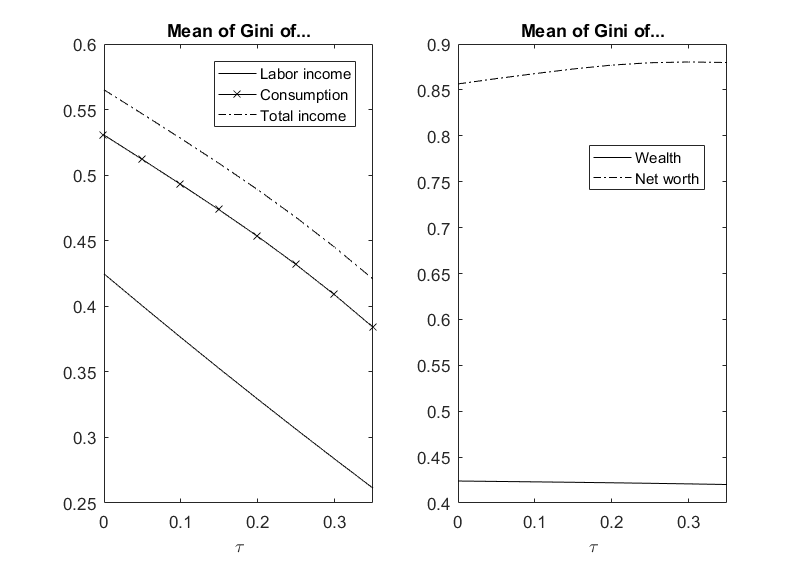
As a robustness check we also run the simulation for the case where the income distribution is described by a Pareto-distribution. We rerun the case for the realistic value of \(a=1.5\) and show that qualitatively the results o changing the tax rate \(\tau\) remain unchanged (cf. Figure 15). In general, the increase in net worth inequality is less pronounced (cf. Figure 16). On the other hand, the wealth inequality in general is higher than in the log-normal specification.

All in all, the redistributive tax is successful in lowering income inequality and thereby also in reducing the number of high-income individuals who engage in potentially destabilizing speculation in the markets for risky assets. On the other hand, the tax can transform a surplus economy in the presence of strong conspicuous consumption into a deficit economy that accumulates large amounts of debt. Moreover, lower income (flow) inequality is accompanied by higher net worth (stock) inequality and therefore has unintended consequences.

Conclusion

This paper argued that higher redistribution by means of taxing labor income can have unintended adverse effects. As the reference level of consumption increases a higher level of debt is required. This not only implies a higher inequality of net worth, but also a potential hazard to financial stability.

Recently some popular advocates (in particular Piketty 2014) proposed a substantial tax on capital (income). In the model at hand this would directly impact on the distribution of net worth and thereby also reduce financial instability as it counteracts the income flow from poor to rich resulting from the debt/claim-relationship. However, there is a well-established literature that opposes any tax on capital income (Atkinson et al. 1976; Judd 1985; Chamley 1986). The key argument of these models is that a tax on the stock of capital distorts the consumption-savings decision in favor of current consumption and decreases the stock of capital leading to lower aggregate output. As we do not have productive capital and growth in our model, this effect cannot be considered in the model at hand.

Note that we only discussed a very stylized and simple quasi-linear taxation and transfer mechanism. A useful extension would be to employ a more realistic real progressive system of taxation and transfers with increasing marginal tax rates. This, moreover, could take advantage of the richness of the ABM methodology not requiring for simple closed form solutions. Another useful extension would be to impute factual micro-data of the distribution of income to quantitatively evaluate policies. We leave this to future research.

References

AITCHISON, J. & Brown, J. A. C. (1957). The Lognormal Distribution, with Special Reference to Its Use in Economics. New York: Cambridge University Press.

ATKINSON, A. B., Piketty, T., & Saez, E. (2011). Top Incomes in the Long Run of History. Journal of Economic Literature, 49(1), 3-71.

ATKINSON, A. B. & Stiglitz, J. E. (1976). The design of tax structure: Direct versus indirect taxation. Journal of Public Economics, 6(1-2), 55-75. [doi:10.1016/0047-2727(76)90041-4]

BLACK, F. (1986). Noise. Journal of Finance, 41(3), 529-43. Board of Governors of the Federal Reserve System (2011). Statistical Database, http://www.federalreserve.gov/apps/fof/.

BORDO, M. D. & Meissner, C. M. (2012). Does inequality lead to a financial crisis? Journal of International Money and Finance, 31(8), 2147-2161. [doi:10.1016/j.jimonfin.2012.05.006]

CARDACI, A. (2014). Inequality, Household Debt and Financial Instability: An Agent-Based Perspective. Imk report 99e, income and wealth distribution in Germany: A macro-economic perspective.

CHAMLEY, C. (1986). Optimal Taxation of Capital Income in General Equilibrium with Infinite Lives. Econometrica, 54(3), 607-22. [doi:10.2307/1911310]

CHIARELLA, C., Died, R., & He, X.-Z. (2009). Heterogeneity, Market Mechanisms, and Asset Price Dynamics. In T. Hens & K. R. Schenk-Hoppé (Eds.), Handbook of Financial Markets: Dynamics and Evolution (pp. 277 - 344). San Diego: North-Holland.

CHIARELLA, C., He, X.-Z., & Hommes, C. (2006). A dynamic analysis of moving average rules. Journal of Economic Dynamics and Control, 30(9-10), 17291753. [doi:10.1016/j.jedc.2005.08.014]

DAVIES, J. B. & Shorrocks, A. F. (2000). The distribution of wealth. In A. Atkinson & F. Bourguignon (Eds.), Handbook of Income Distribution, volume 1 of Handbook of Income Distribution chapter 11, (pp. 605-675). Amsterdam: Elsevier.

DIAMOND, P. & Saez, E. (2011). The Case for a Progressive Tax: From Basic Research to Policy Recommendations. Journal of Economic Perspectives, 25(4), 165-90. [doi:10.1257/jep.25.4.165]

DOEPKE, M. & Schneider, M. (2006). Inflation and the Redistribution of Nominal Wealth. Journal of Political Economy, 114(6), 1069-1097.

D’ORLANDO, F. & Sanfilippo, E. (2010). Behavioral foundations for the Keynesian consumption function. Journal of Economic Psychology, 31(6), 1035-1046. [doi:10.1016/j.joep.2010.09.004]

DUESENBERRY, J. (1949). Income, saving and the theory of consumer behavior. Cambridge, MA: Harvard University press (Oxford University press).

FISCHER, T. (2012). News Reaction in Financial Markets within a Behavioral Finance Model with Heterogeneous Agents. Algorithmic Finance, 1(2), 123-139.

FISCHER, T. (2013). Inequality and Financial Markets - A Simulation Approach in a Heterogeneous Agent Model. In A. Teglio, S. Alfarano, E. Camacho- Cuena, & M. Gines-Vilar (Eds.), Managing Market Complexity - The Approach of Artificial Economics, Lecture Notes in Economics and Mathematical Systems, volume 662 (pp. 79-90). Springer.

FISCHER, T. (2015). Inequality and Financial Stability in an Agent-Based Model. Dissertation, Technische Universität Darmstadt.

FRIEDMAN, M. & Friedman, R. (1962). Capitalism and Freedom. Economics Politics. Chicago: University of Chicago Press.

HOMMES, C. & Wagener, F. (2009). Complex Evolutionary Systems in Behavioral Finance. In T. Hens & K. R. Schenk-Hoppé (Eds.), Handbook of Financial Markets: Dynamics and Evolution (pp. 217 - 276). San Diego: North-Holland. [doi:10.1016/B978-012374258-2.50008-7]

JUDD, K. L. (1985). Redistributive taxation in a simple perfect foresight model. Journal of Public Economics, 28(1), 59-83.

KÖNIG, N. &Größ, I. (2014). Catching up with the Joneses and Borrowing Constraints: An Agent-based Analysis of Household Debt. Macroeconomics and Finance Series 2014.04, Hamburg University, Department Wirtschaft und Politik.

KUMHOF, M., Rancière, R., & Winant, P. (2015). Inequality, Leverage, and Crises. American Economic Review, 105(3), 1217-45.

LUX, T. (2009). Stochastic Behavioral Asset-Pricing Models and the Stylized Facts. In T. Hens & K. R. Schenk-Hoppé(Eds.), Handbook of Financial Markets: Dynamics and Evolution (pp. 161 - 215). San Diego: North-Holland. [doi:10.1016/B978-012374258-2.50007-5]

MANSKI, C. F. & McFadden, D. (1981). Structural analysis of discrete data with econometric applications. Cambridge, Mass: MIT Press.

MERTON, R. C. (1971). Optimum consumption and portfolio rules in a continuous-time model. Journal of Economic Theory, 3(4), 373-413. [doi:10.1016/0022-0531(71)90038-X]

OECD (2012). Statistical database of the Organisation for Economic Co-Operation and Development (last accessed on 11/11/2014)

OKUN, A. (1975). Equality and Efficiency: The Big Tradeoff. G - Reference, Information and Interdisciplinary Subjects Series. Washington, D.C.: Brookings Institution.

PARETO, V. (1896). Cours d’Economie Politique. Geneve: Droz.

PIKETTY, T. (2014). Capital in the twenty-first century. Boston: Harvard University Press. [doi:10.4159/9780674369542]

RAJAN, R. (2010). Fault lines : how hidden fractures still threaten the world economy. Princeton: Princeton University Press.

REICH, R. B. (2010). Aftershock : the next economy and America’s future. Alfred A. Knopf, New York, 1st edition.

ROINE, J., Vlachos, J., & Waldenström, D. (2009). The long-run determinants of inequality: What can we learn from top income data? Journal of Public Economics, 93(7-8), 974-988.

SAEZ, E. & Zucman, G. (2016). Wealth Inequality in the United States since 1913: Evidence from Capitalized Income Tax Data. The Quarterly Journal of Economics, 131(2), 519-578. [doi:10.1093/qje/qjw004]

SHORROCKS, A. (1982). The Portfolio Composition of Asset Holdings in the United Kingdom. Economic Journal, 92(366), 268-84.

WOLFF, E. N. (2013). The Asset Price Meltdown, Rising Leverage, and the Wealth of the Middle Class. Journal of Economic Issues, 47(2), 333-342.