
Introduction
The most shocking economic crisis of this century took place on 2008 after Lehman Brothers bankruptcy. This unexpected event has reinforced the interest on systemic risk in the scientific community, and different studies on the stability, resilience, and optimal structures of financial systems have arisen as an attempt to describe the causes of the present crisis and also to prevent possible future financial shocks (see Gai & Kapadia 2010; Haldane & May 2011; Allen et al. 2012; Mishkin 2012; Acemoglu et al. 2013, among many others). The resilience of the financial system under different kinds of shocks, however, was an important subject of research long before the last financial crisis. Liquidity shocks, contagion, or the role of interbank market in the propagation of liquidity failures are among the most studied phenomena in systemic risk (see, for example, Allen & Gale 2000; Freixas et al. 2000; Ashcraft & Duffie 2007). In particular, the interbank market plays a crucial role in the liquidity needs of financial institutions. They often ask for punctual financial resources to address their liquidity needs, and the complex structure of the interbank market, with a huge number of institutions involved and an intense transaction activity, is usually able to absorb the perturbations caused by the default of a bank (Mishkin 2007). However, the conditions under which interbank lending markets can attenuate liquidity perturbations remain elusive.
Nowadays, banks use electronic markets for multilateral trading in the interbank market, which makes circulation of liquidity more efficient, like classical clearing houses did in the past century. The first electronic market for interbank deposits was e-MID, born in 1990 from the Bank of Italy and the Italian banking community. Since then, large-value payment (LVP) systems have evolved and banks can now have access to many facilities to ease interbank trading[1]. These LVP systems allow the collection of a database of transactions that can be analyzed in order to shed more light into the dynamics of the interbank market, to establish proper regulations that minimize systemic risk.
To this end, attempts to apply network theory to the analysis of trading data have proliferated among researchers and central banks (ECB 2010, is an example of the interest shown by high institutions in this interdisciplinary area). In this direction, the work by Boss et al. (2004) was “the first to provide an empirical analysis of the structural features of a real-world interbank network using concepts from modern network theory”. Results from the analysis of realized interbank transactions could be compared with other empirical data and could be used for modeling interbank contagion processes. Other investigations of this kind using data from other LVP systems are Soramäki et al. (2007); Iori et al. (2008); Bastos e Santos & Cont (2010); Martínez-Jaramillo et al. (2012); Fricke & Lux (2015).
As we show below, the similarity between the measured properties of these LVP systems suggests that, however heterogeneous the systems might seem, they share a common structure that could be modeled or reproduced as a first step to find a source of policy recommendations and improve interbank market stability. This paper is the first that collects and compares empirical results from interbank markets around the world in order to do that.
The road map proposed in the literature for applying network theory to the interbank market is the following. Every loan agreement in the interbank market is a transaction where an amount is settled between a lender and a borrower at some interest rate (Mishkin 2007). Each transaction can then be represented by a directed link with a weight which is the amount of the loan. Intra-day analysis of the interbank market shows a large volume of transactions per day. Interbank networks can thus be constructed from daily transactions or from the aggregation of these transactions over longer periods.
The main network property transferred from empirical interbank data to theoretical works is the distribution of the number of borrowers and lenders (in the network literature, these quantities are known as in- and out-degree distributions; see a rigorous definition in Appendix A). Empirical studies reveal that the degree distribution appears to be long tailed[2]. As a result, most theoretical works have dealt with static interbank networks, therefore assuming fixed in time borrower-lender relationships, even in situations of financial distress (Iori et al. 2006; Gai & Kapadia 2010; Loepfe et al. 2013; Georg 2013), in order to study default cascades. Despite the value of these investigations, this assumption could lead to erroneous conclusions in the assessment of system resilience since, as explained above, interbank networks are usually the aggregated result of high-frequency dynamic trading.
Since the market structure emerges endogenously, it should be obviously modeled as an agent-based dynamic process, opposed to a static, exogenous network approach. This paper proposes a minimal, stochastic, consistent agent-based model of the inter-bank network, which can be used as a benchmark for both theoretical models and empirical data. Our modeling approach is based on data from the balance sheets of banks in the Bankscope database, namely the ones relative to the total assets, the inter-bank assets and the interbank liabilities of each bank at the end of the year. A detailed statistical analysis of this database, together with simple hypotheses regarding the way in which transactions take place, leads to our model. The model is minimal as it makes simple assumptions and does not define complicated actions between the agents. It is also stochastic as our lack of information on agent strategies and transaction data is supplied with randomness. The main assumption of the model is that interbank assets and liabilities are to be compensated, as far as possible, in each trading round. Although admittedly simple, our model is consistent as it reproduces qualitatively the basic topological network properties measured in real LVP systems.
The paper is organized as follows: in Section 2 we describe the Bankscope dataset and analyze the observed distributions and correlations of interbank assets, liabilities and total assets. In Section 3 we present the network model, which involves three different scenarios for assets and liabilities generation, as well as the way in which links (loans) are drawn depending of bank positions. In Section 4 we show that our minimal model is able to capture the basic structure reported on empirical studies, and we end this contribution with several conclusions and prospects (Section 5).
Data Analysis
This work relies on data from the Bankscope database[3], which gathers information of financial statements, ratings and intelligence of over tens of thousands of banks around the world. We retrieved records from 32505 banks, which consist of end-of-year data from 2008 to 2015, both inclusive, regarding the size of the banks (total assets, TA), interbank assets (loans and advances to banks, LAB) and interbank liabilities (deposits from banks, DB). We exclude central banks and clearing houses from the analysis, as they are not driven by the same dynamics in contagion processes as the rest of institutions do.
The large majority of the records have positive data in both interbank assets and liabilities. The amount of interbank assets that belong to records with no DB only represents the 2.44% of all the LAB, and the amount of DB from records with no LAB is the 0.42% of the total.
We thus analyze data with strictly positive TA, LAB and DB, which rendered 51269 records to analyze along the 2008-2015 period (the same institution can be recorded repeatedly in different years). Systematically, the overall amount of interbank liabilities exceeds the total interbank assets, as can be seen in Table 1, which unveils the existence of other lenders not reported in the database. The interbank market that we can model with these data is, therefore, an open system embedded in the world interbank market.
| Year | IB assets (\(\times 10^{12}\) USD) | IB liabilities (\(\times 10^{12}\) USD) | Net IB (\(\times 10^{12}\) USD) | Min. external IB (%) |
| 2008 | 16.59 | 20.68 | -4.09 | -24.62 |
| 2009 | 17.12 | 20.73 | -3.61 | -21.08 |
| 2010 | 13.81 | 18.29 | -4.48 | -32.46 |
| 2011 | 13.95 | 18.23 | -4.28 | -30.67 |
| 2012 | 14.3 | 17.75 | -3.46 | -24.18 |
| 2013 | 14.36 | 18.09 | -3.74 | -26.02 |
| 2014 | 12.66 | 16.56 | -3.9 | -30.81 |
| 2015 | 2.93 | 3.15 | -0.22 | -7.58 |
Figure 1 shows some interesting features of the distributions of TA, LAB and DB (see caption for details). Since LAB is part of TA, LAB < TA must hold for each entity and, if it is solvent, the same is true for DB < TA, which make distributions to be far from bivariate log-normal distributions, although marginal distributions might seem close to log-normal functions.
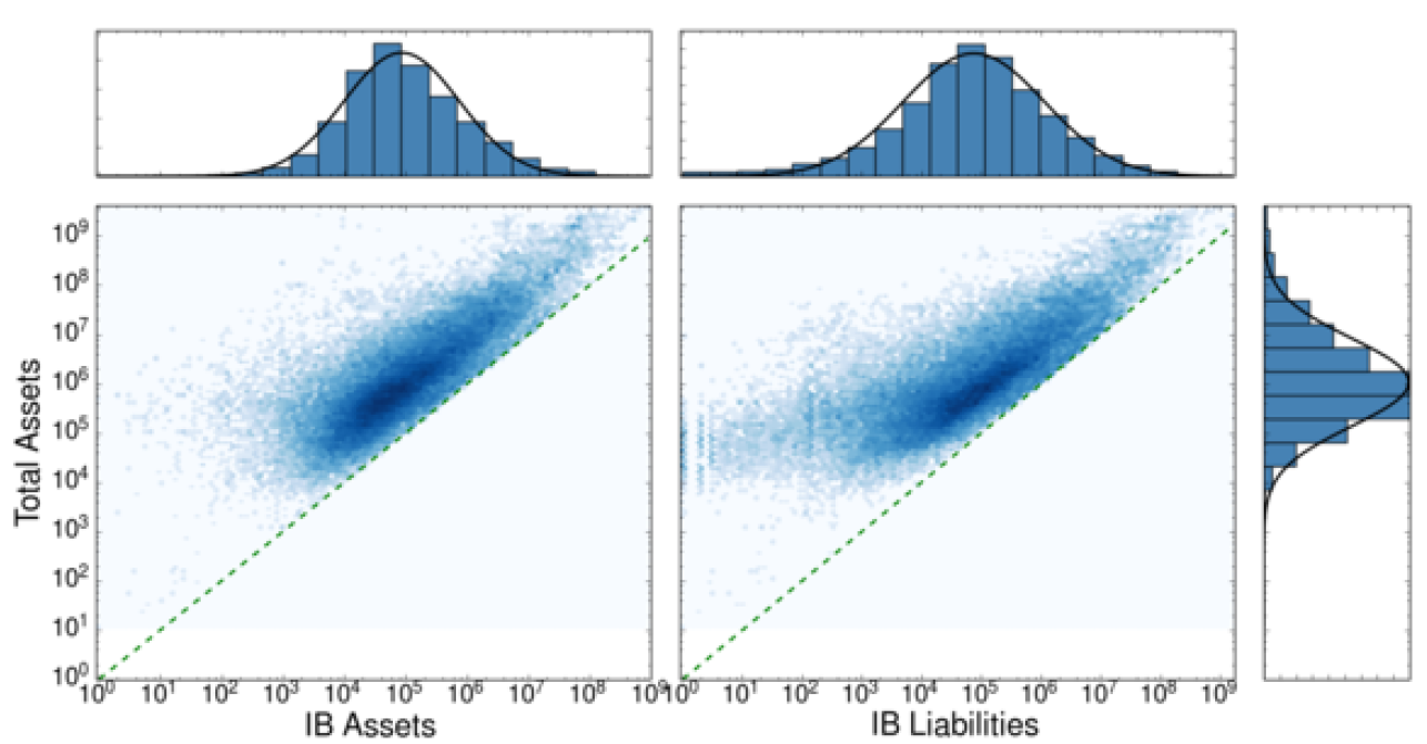
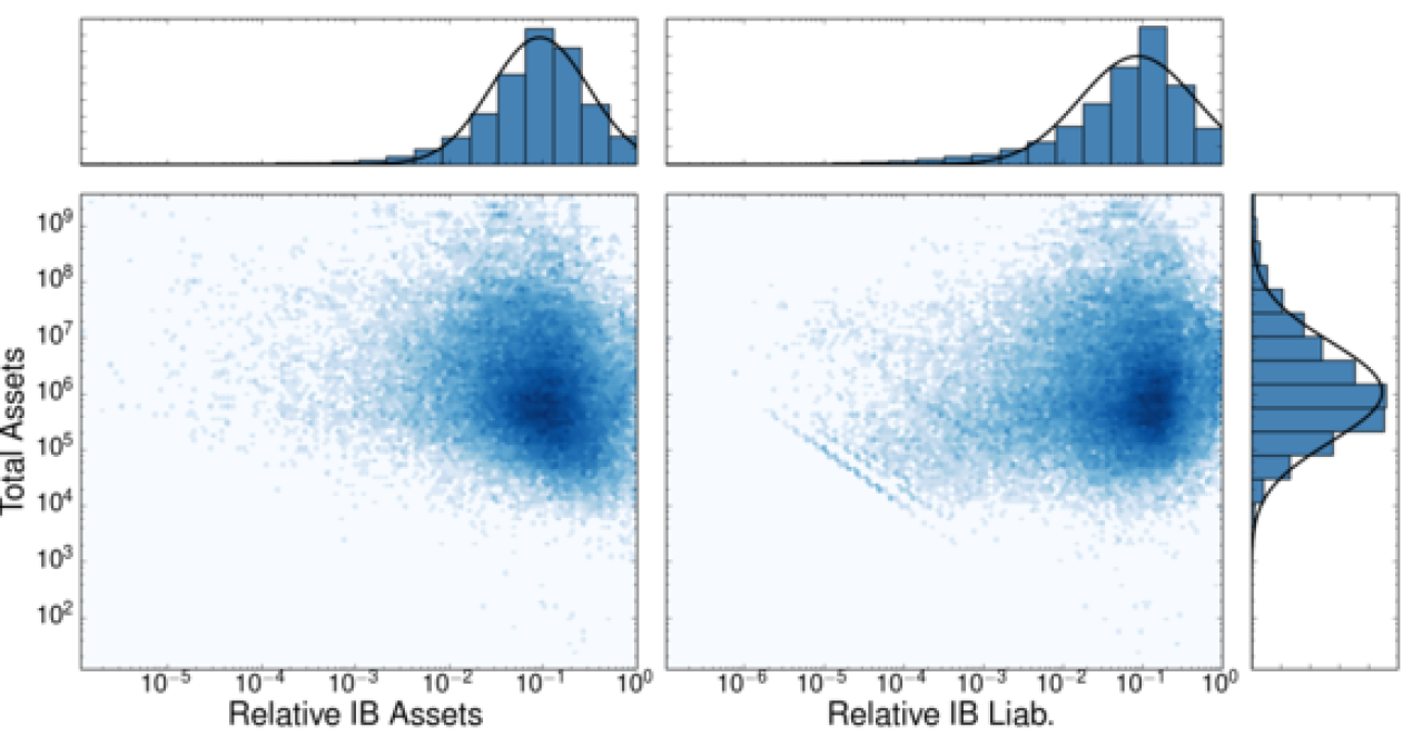
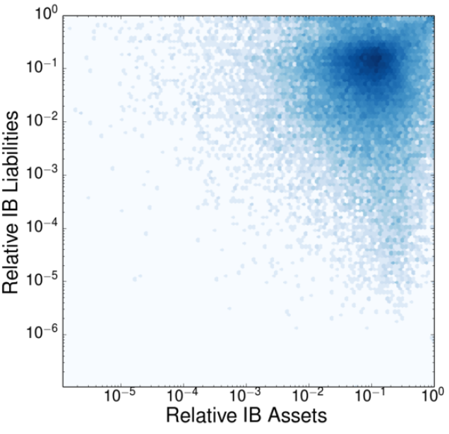
In order to soften the strong correlation between TA and LAB (DB), we introduce the relative variable \(x\) = LAB/TA (\(y\) = DB/TA), whose distribution is shown in Figures 2 and 3. As a side effect, the truncation of the bivariate distributions is apparent in the marginal distributions of \(x\) and \(y\). More importantly, we observe that correlations between TA and the relative variables \(x\), \(y\) are weak (see Figure 2). The linear correlation analysis between scaled variables is detailed in Table 2.
| Linear model in log-log scale | r2 | p-value |
| Relative IB assets (\(x\)) vs. total assets | 0.042 | 0 |
| Relative IB liabilities (\(y\)) vs. total assets | 0.012 | 0 |
| Relative IB assets (\(x\)) vs. relative IB liabilities (\(y\)) | 0.00 | 0.051 |
Network Model
In this section we define the model that generates interbank networks. The set of TA, LAB and DB data described in Section 2 allows for the definition of our model of the interbank system as follows.
We consider a banking system formed by \(N\) banks. Bankscope reports the balance sheets of financial institutions at December, 31st each year. We used these yearly data as a proxy for the positions of banks in the interbank market at any day. The position of bank \(i\) (\(i=1,\ldots,N\)) in the interbank market is defined by variables \((a_i, l_i)\), where \(a_i\) stands for the interbank assets (LAB) and \(l_i\) is the amount of interbank liabilities (DB) of the bank. As shown in Figure 1, these variables cannot be drawn independently of the size (TA) of bank \(i\), \(z_i\).
Assets and liabilities generation
The triplet \((x_i, y_i, z_i)\), with \(x_i=a_i/z_i\)and \(y_i=l_i/z_i\), is the set of random variables used to generate \(a_i\) and \(l_i\) for bank \(i\). We use relative variables instead of drawing directly \(a_i\) and \(l_i\) because relative variables are weakly correlated to bank sizes. In order to assess the importance of variable correlations, we used in the simulations three different ways of generating the triplets \((x_i, y_i, z_i)\).
Full correlation (FC). For each bank \(i\) we sample \(z_i\) from to empirical marginal distribution of bank sizes, \(P(z)\), obtained from the Bankscope dataset. Then we calculate empirical joint conditional probabilities \(P(x, y\vert z_i)\) and, from them, draw the pairs \((x_i, y_i)\). Conditional probabilities are calculated as the distributions obtained by restricting to all bank sizes \(z_i\) that verify \(0.95z\le z_i\le 1.05 z\). This method generates samples of the joint distribution \(P(x,y,z)\) of the original data. Algorithm 1 describes the details of this method.
Half correlation (HC). This case also uses the empirical marginal distribution of bank sizes and, for each \(z_i\), we calculate conditional empirical probabilities \(P(x\vert z_i)\) and \(P(y\vert z_i)\) from the Bankscope dataset to independently draw variables \(x_i\) and \(y_i\). Here we are assuming zero correlation between variables \(x\) and \(y\). This method generates samples with the same joint, marginal distributions \(P(x,z)\) and \(P(y,z)\) as the original data.
No correlation (NC). In this case, \(x_i\), \(y_i\) and \(z_i\) are independently drawn according to the marginal empirical distributions \(P(x)\), \(P(y)\), and \(P(z)\) obtained from the Bankscope database. Here we assume zero correlation between all variables.
Algorithm 1 Pseudocode for the random generator with full correlation.
▷ Global variables: datax – Empirical list of relative interbank assets (LAB/TA) of banks datay – Empirical list of relative interbank liabilities (DB/TA) of banks dataz – Empirical list of sizes (TA) of banks 1: function initialize(file) 2: datax, datay, dataz = loadDataFromFile(file) 3: end function 4: function generateBankSizes(size) 5: ta = randomSample(dataz, size) 6: return ta 7: end function 8: function generateInterbankFC(totalAssets) 9: lab = emptyList( ) 10: db = emptyList( ) 11: for each z in totalAssets do 12: indices = List of indices of dataz whose values are between 0.95z and 1.05z 13: i = randomChoice(indices) 14: appendToList(lab, datax[i]*z) 15: appendToList(db, datay[i]*z) 16: end for 17: return lab, db 18:end function
Algorithm 2 Pseudocode of the random generator of the interbank positions in the half correlated method.
8: function generateInterbankHC(totalAssets) 9: lab = emptyList( ) 10: db = emptyList( ) 11: for each z in totalAssets do 12: indices = List of indices of dataz with values between 0.95z and 1.05z 13: i = randomChoice(indices) 14: appendToList(lab, datax[i]*z) 15: j = randomChoice(indices) 16: appendToList(db, datay[j]*z) 17: end for 18: return lab, db 19:end function
Algorithm 3 Pseudocode of the random generator of interbank positions in the uncorrelated method with empirical marginal distributions.
8: function generateInterbankNC(totalAssets) 9: lab = emptyList( ) 10: db = emptyList( ) 11: for each z in totalAssets do 12: x = randomChoice(datax) 13: appendToList(lab, x*z) 14: y = randomChoice(datay) 15: appendToList(db, y*z) 16: end for 17: return lab, db 18:end function
Random network generation
The positions of interbank assets and liabilities of each bank were generated with one of the methods mentioned above. We do not try to model how these quantities arise, only the way in which a network of interbank interactions can be constructed from them. As we show in the pseudocode below, the rationale behind our method to generate the interbank network amounts to randomly compensate the differences between assets and liabilities through a number of loans. At the end of the simulation, a network with all the interbank interactions is obtained.
Algorithm Pseudocode of the algorithm used to simulate the interbank network.
▷ Global variables: IBassets – List of interbank assets IBliabs – List of interbank liabilities G – Graph representing the interbank network 1: function chooseLenders(borrower, L) ▷ Given a borrower bank with liquidity needs and a list of available banks with an excess of liquidity, this function chooses sequentially at random the lenders from the available banks and calculates the loan by using all the available resources from the lender, if necessary, until the liquidity needs of the borrower bank are fulfilled. Self loans are not allowed. ▷ Inputs: borrower – The borrower bank L – List of banks with strictly positive IBassets ▷ Returns: lenders – List of all the banks that lend liquidity to the borrower amounts – List of loans, one for each lender 5: lenders = emptyList( ) 6: amounts = emptyList( ) 7: while L not empty and L != oneElementList(borrower) do 8: lender = randomChoice(L, exclude = borrower) 9: appendToList(lenders, lender) 10: if IBliabs[borrower] > IBassets[lender] then 11: appendToList(amounts, IBassets[lender]) 12: IBliabs[borrower] = IBliabs[borrower] - IBassets[lender] 13: IBassets[lender] = 0 14: removeFromList(L, lender) 15: else 16: appendToList(amounts, IBliabs[borrower]) 17: IBassets[lender] = IBassets[lender] - IBliabs[borrower] 18: IBliabs[borrower] = 0 19: break 20: end if 21: end while 22: return lenders, amounts 23:end function 24:function networkGeneration( ) ▷ This function chooses sequentially at random all the banks with liquidity needs (borrowers). For each borrower, it calls to chooseLenders to get the list of lenders and amounts lent, and then it adds the corresponding links, transactions and loans to network G (global variable). Links go from borrowers to lenders. 25: L = list of all banks 26: B = shuffle(list of all banks) 27: for each borrower in B do 28: lenders, amounts = chooseLenders(borrower, L) 29: for each lender, amount in (lenders, amounts) do 30: if not existsLink(G, borrower, lender) then 31: addLink(G, borrower, lender) 32: end if 33: addTransaction(G, borrower, lender) 34: addLoan(G, borrower, lender, amount) 35: end for 36: end for 37:end function 38:function simulation(N, nR, model) ▷ Inputs: N – Number of banks in the interbank market nR – Number of rounds to generate the interbank network model – FC, HC or NC model used to generate bank positions ▷ Initialize variables 39: bankSizes = generateBankSizes(N) ▷ Generates the total assets of banks 40: G = initializeNetwork(N) 41: IBassets0, IBliab0 = generateInterbank(bankSizes, model) ▷ nR rounds of trades, aggregating data in G in each round 42: for n = 1 to nR do 43: IBassets = multiplyList(IBassets0, 1/nR) 44: IBliab = multiplyList(IBliab0, 1/nR) 45: networkGeneration( ) 46: end for 47:end function
In brief, our algorithm for daily network generation works as follows. First we generate \(N\) random bank sizes and, according to the rules defining models FC, HC or NC, we draw their relative bank positions \((x_i,y_i,z_i)\). From these we calculate the pairs \((a_i,l_i)\) of assets and liabilities for each entity. At the beginning of the algorithm, these quantities represent the liquidity excess and the liquidity needs of each bank, which the algorithm will transform into loans and advances to banks (interbank assets) and deposits from banks (interbank liabilities). In order to do that, along a given number of \(n_R\) rounds, we run over the set of borrower banks (i.e., those with \(l_i>0\)) and draw directed links from borrowers to available lenders (those with \(a_i>0\)) at random. Given a borrower \(i\) and a lender \(j\), if the lender can cover all the liabilities of the borrower at the transaction attempt (i.e., if \(a_j\ge l_i\)), then a transaction covering the total amount takes place, the lender's surplus is updated to be \(a_j-l_i\) (this amount forms a loan to be included in the balance sheet of bank \(j\) as an asset and of bank \(i\) as a liability), and the liquidity needs of the borrower are set to zero. If the condition \(a_j\ge l_i\) does not hold, an amount \(a_j\) is lent from lender to borrower and surpluses and deficits are updated accordingly (lender's surpluses to zero and borrower's liquidity needs to \(l_i-a_j\)), requiring the borrower to try to compensate its liquidity needs from another lender chosen at random from all the available lenders. In each network generation, the order in which transactions are established is purely random. Networks are aggregated over the total number of rounds. Our model is basically null with regard to the identities of banks that are interacting with each other. The only rule of this model is to try to compensate, by making liquidity needs of borrowers equal to zero, as many bank debts as possible.
Since interbank positions are randomly drawn, the sum of all interbank assets does not necessarily equals the overall aggregation of interbank liabilities. This is due to the fact that available trade data in the Bankscope database provides only a partial picture, since there are other financial institutions not reported in the database that contribute to the global interbank market.
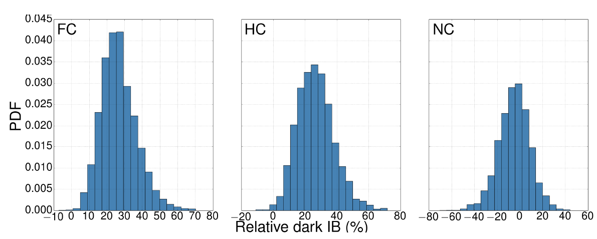
The distribution of the relative size of this “dark market” is shown in Figure 4 (see caption for details), whereas Table 3 provides some quantitative indicators of the distribution shape. We observe that correlated models (both FC and HC) systematically generate, in agreement with Table 1, interbank markets with an excess of liabilities that must be compensated by the dark interbank market. Model NC, however, ignores correlations and generates on average the same excess of interbank assets and liabilities. These differences arise because relative assets and liabilities (\(x\), \(y\)) are weakly correlated with bank sizes (\(z\); see the two first rows in Table 2) but are multiplied by \(z\) to get absolute values for interbank assets and liabilities afterwards. Such scaling with size amplifies the initially small differences in the distributions of relative interbank assets and liabilities generated according to this model (note that FC and HC models assume these correlations to be non-zero). Importantly, Table 3 shows that the distributions for the FC and HC models are almost identical and we can, therefore, assume no correlation between the relative variables \(x\) and \(y\) but non-zero correlation with bank sizes. In Appendix B we get the same picture in this respect after the analysis of network properties. Therefore, in the rest of this contribution we use FC and HC models indistinctly, and disregard the NC model.
The empirical networks reported in this manuscript are associated to political regions with a large historical background. Banks probably tend to trade among each other within the same region and, if they cannot fulfill their liquidity requirements, trade with other institutions outside their countries. This propensity to intra-region interactions surely leads to a community structure within the global interbank network that our model does not account for, not at least explicitly. However, we can manage to overcome that issue by simulating interbank networks with the same size as the empirical ones which we compare our model with. This way, our model reproduces the regional trading preferences of financial institutions by trying to cancel out each other's interbank positions between them and, when no more lending within the modeled network is possible, by resorting to the external interbank market. Therefore, the existence of the dark market outside the model is clearly justified.
| Model | Dark IB (\(\times 10^{12}\) USD) | Rel. dark IB (%) | ||||
| mean | std | mean | std | \(\alpha\)2.5 | \(\alpha\)97.5 | |
| FC | 3.72 | 1.30 | 26.75 | 10.11 | 9.34 | 49.72 |
| HC | 3.80 | 1.56 | 26.62 | 11.55 | 6.74 | 51.59 |
| NC | 1.12 | 3.04 | 5.21 | 13.87 | 33.52 | 21.39 |
As bank positions are obtained from data and the size of the network is fixed, our “minimal” model has only one adjustable parameter, which is the number of trading rounds in a single day, \(n_R\). Our model assumes that interbank trading is divided into an (average) number of trading rounds per day, fixed for all banks, that determines the average amount of money lent or borrowed by each bank —the larger the number of rounds the lesser the amount. The effect of that parameter in model outcomes is explained in detail in Appendix B, along with a description of how some topological properties of our model networks depend on network size, \(N\), the number of trades per day, \(n_R\), and the correlation method used (FC or HC).
Our algorithm for interbank network generation makes some unrealistic assumptions. Borrower banks choose at random lender banks, regardless the loan interest, historical background or previous lenders they chose. On the other hand, lenders always accept the loans using all of their potential resources regardless of the amount requested or the borrower rating. Our model, therefore, considers no prices, no strategic preferences, nor risk aversion. However, as shown below, and despite these assumptions, comparison with real data is quite good. Posterior refinements of the model could incorporate some of these features, although it is remarkable that such a minimal model performs considerably well when confronted to empirical data reported in the literature.
In the following section we analyze the similarities of model networks with empirical network magnitudes measured in the interbank literature.
Comparison with Empirical Data
In this section we test model predictions against data reported for empirical interbank networks. Comparison with empirical data is not a straightforward process. Since there is no standard procedure in data acquisition, network analysis depends heavily in the way interbank assets and liabilities are defined, the maturities that are considered, or the network aggregation across time ranges. For instance, the works by Iori et al. (2008) and Fricke & Lux (2015) only took into account overnight loans, whereas we consider all maturities. In addition, these two contributions report important differences in network properties, although they both studied the Italian interbank market over different periods. These differences point to the degree of accuracy of the data definition and retrieval.
Moreover, the way network properties are presented in the papers analyzed here also affects the accuracy of our data acquisition procedure. We used a digitization tool (Rohatgi 2015) to acquire reported data from article figures. When fat-tailed probability density functions (PDF) are depicted in logarithmic scale, usually the tail of the distribution is very noisy and data acquisition can be inaccurate. In those cases, only the left-most part of the distribution is reliable when transforming it into a complementary, cumulative distribution function (CCDF) defined as the probability \(P(X\ge x)\). Similarly, reported CCDF data in logarithmic scale may yield inaccurate PDF plots. We have used CCDFs in order to compare model outcomes with real observations, as they have less noise in the right tail. Notice also that any CCDF must be equal to 1 at the lowest value of the variable, although this is not the case in some empirical CCDFs reported (see below), which rises some concerns about the accuracy of the data.
Table 4 shows some features of the empirical data used for model validation, namely: the country, the period studied, the network size, the Interbank market features considered, and the set of analyzed network properties. The table illustrates the heterogeneity in data definitions, measured network properties and distribution formats (PDF, CCDF) used to present them. Thus, a thorough comparison of any model with these data becomes a hard task. Differences in the properties between our model and empirical data can arise because of model assumptions, because the Bankscope data used to generate model networks differs greatly from those used in empirical studies or, as mentioned above, because of errors arising in data acquisition from figures.
As a consequence, we have not tried to fit simultaneously a subset of empirical network properties. Instead, we show how our minimal model reproduces qualitatively and, sometimes even quantitatively, some of the properties observed in empirical works. This basically means that a random sampling of interbank positions from Bankscope, a simple rule to compensate interbank assets and liabilities, and a single tunable parameter \(n_R\) (the average number of daily trading rounds) is enough to re produce global trends in network properties. For that purpose, we have fixed network sizes to match those of empirical networks and considered a number of trades per day \(n_R\) that yielded better agreement with reported network properties. As for the correlation method, since both the FC and HC methods used to produce interbank positions yield to similar outcomes, the comparison with empirical data has been conducted using only the HC model.
| Reference | Country | Period | Network size | Interbank market features considered | Network properties |
| Boss et al. (2004) | Austria | 2000-2003 | 900 | Austrian interbank market based on Austrian Central Bank data Links go from borrowers to lenders Quarterly single month periods | Figure 1(b): Exposures (histogram*) Figure 3(a): In-degree (histogram*) Figure 3(b): Out-degree (histogram*) |
| Soramäki et al. (2007) | USA | 2004Q1 | 5086±128 | Interbank payments transferred between commercial banks over the Fedwire® Funds Service Links go from borrowers to lenders Daily networks | Figure 8: Out-degree (PDF*) Figure 9: Nearest successor out-degree vs. out- degree Figure 11 (top, right): Out-transactions (PDF*) Figure 11 (bottom, left): Loan sizes (PDF) Figure 11 (bottom, right): IB assets (PDF) |
| Iori et al. (2008) | Italy | 1999-2002 | 215-177 | All the overnight e-MID transactions Links go from lenders to borrowers Daily networks | Figure 5 (top, right): In- and out-transactions, 2002 Figure 5 (bottom, right): In- and out-degree, 2002 (DDF) Figure 9: Average nearest neighbors degree vs. degree (undirected) |
| Bastos e Santos & Cont (2010) | Brazil | Nov-2008 | 2409 | Fixed-income instruments, borrowing and lending, derivatives and foreign exchange Links go from borrowers to lenders One single-day network | Figure 3: In-degree (CCDF) Figure 4: Out-degree (CCDF) Figure 6: Exposures (CCDF) Figure 7: Clustering vs. degree (undirected, scatter plot) |
| Martínez-Jaramillo et al. (2012) | Mexico | 2005-2010 | 27-40 | All the possible deposits, credits and loans, including credit lines, and excluding FX exposures for the banks which use the services provided by the Continuous Linked Settlement Bank, obtained from the SPEI data Undirected links Daily networks | Figure 10 (a): Degree (CCDF) Figure 10 (b): Exposures (CCDF) Figure 12 (a): Average nearest neighbors degree |
| Fricke & Lux (2015) | Italy | 1999-2010 | NA | Networks based on the Italian e-MID data for overnight loans Links go from lenders to borrowers Daily and quarterly networks | Figure 7 (left): In-degree (CCDF) Figure 7 (center): Out-degree (CCDF) Figure 13 (left): In-transactions (CCDF) Figure 13 (center): Out-transactions (CCDF) |
Figure 5 shows how our model can reproduce empirical in-degree distributions. Most of the empirical interbank networks exhibit a long-tailed degree distribution, which is recovered by our model. Other authors (Iori et al. 2008; Fricke & Lux 2015) report distributions with shorter tails (Figure 5); in those cases our model could be used to reproduce in-degrees at certain intermediate ranges. The same comments apply for out-degree distributions.
We observe in Figure 5 (bottom panels) that empirical in- and out-transactions for the Italian e-MID interbank market (Iori et al. 2008; Fricke & Lux 2015) differ each other by one order of magnitude. Our model, nevertheless, reproduces qualitatively the Italian interbank market and quantitatively the case of the USA (Soramäki et al. 2007), see the panel for out-transactions.
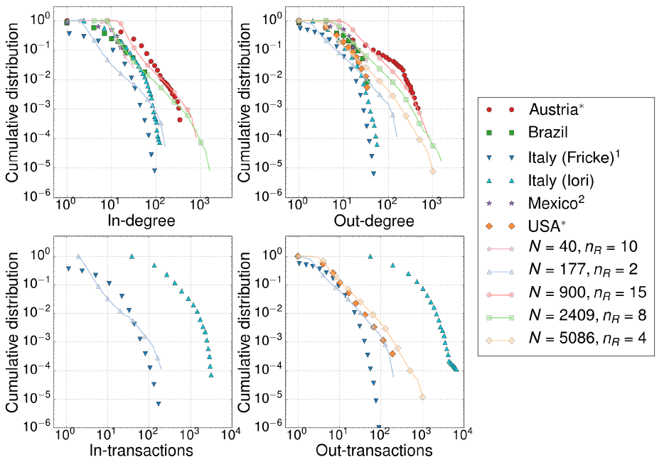
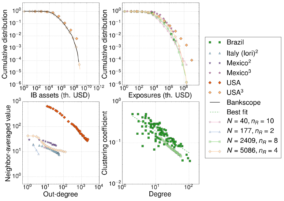
As expected, the distribution of total interbank assets (which coincides with the distribution of LAB in the Bankscope database) is recovered by our model, and agrees very well with the empirical data of the USA interbank network reported by Soramäki et al. (2007) — see Figure 6. Other properties very well reproduced by our model are the distribution of exposures (the total amount lent between each pair of banks) in Mexico (Martínez-Jaramillo et al. 2012), USA (Soramäki et al. 2007) and Brazil networks (Bastos e Santos & Cont 2010), as well as the clustering coefficient of the Brazilian inter-bank market. The empirical disassortativity observed in Mexico (Martínez-Jaramillo et al. 2012) and Italy (Iori et al. 2008) are qualitatively captured by our simple model, although for the USA market (Soramäki et al. 2007) predictions depart largely from empirical observations.
Conclusions
In this contribution we have introduced a network model for interbank markets using a simple agent-based algorithm for generating daily, temporal transaction networks. To that end, we have used interbank positions of financial institutions from end-of-year balance sheets of the Bankscope database, which is available for researchers in many institutions world wide.
Our model is based on three variables to define bank positions, namely: total assets, interbank assets and interbank liabilities. An analysis of these variables shows that the correlation between interbank assets and liabilities emerges from the scaling of these quantities with bank sizes (total assets). Another key ingredient in our model is randomness. Banks with liquidity needs borrow from banks with liquidity surpluses uniformly at random until their needs are fulfilled, after a number of repeated transaction attempts. Financial institutions do not work that way, obviously. Our model lacks of other realistic features, such as profit maximization, risk aversion or other strategic decisions. However, the networks generated fit qualitatively basic empirical properties reported in the literature. This result yields important implications. First, our model could be used as a benchmark of the interbank market, a null model that can be compared with more realistic models. Here we have analyzed basic topological properties and we have shown that the model qualitatively reproduces them on the basis of very simple rules. This methodology would allow to discriminate magnitudes and mechanisms that are relevant to interbank systems from others that can be explained by our simple model. For example, we have not analyzed how our model accounts for the local, motif structure of empirical interbank networks (Squartini et al. 2013). Given that our model captures basic properties itself, it could be used as a null model to test the degree of significance of the observed frequencies of motifs in real networks. We believe that this benchmark is of paramount importance in the development of interbank network modeling, as it rules out models that may comply with some data from real LVP systems whose results do not significantly differ from those of our model. A second implication is that the properties usually measured in empirical networks can be accounted through a minimal set of basic rules, so other magnitudes are to be analyzed in forthcoming studies. More complex, realistic models replicating the properties exposed in this manuscript with the same accuracy as ours cannot be considered better, unless additional quantities are further considered. These new properties could be used to reject our model and to test more realistic assumptions. Either way, it would mean a step forward in the knowledge of interbank networks as a way to study, for instance, important aspects that cause systemic or liquidity risks.
We followed a top-down approach to generate model networks. Starting from a set of interbank assets and liabilities, our basic assumption to draw links in model networks is the requirement that interbank assets and liabilities compensate each other through interbank transactions. In other contexts, a simple rule like this has been used, for example, to generate good approximations for predator-prey interaction networks in ecology (Williams & Martinez 2000; Camacho et al. 2002; Stouffer et al. 2006; Capitán et al. 2013) or contact networks in language biogeography (Capitán et al. 2015; Capitán & Manrubia 2015). However, the knowledge of actual daily loans in the interbank market would allow for a bottom-up approach. In that case, fine-tuned models considering individual strategical decisions that generate each transaction between banks could be developed. Trading preferences, according to asymmetric differences arising in actual bank transactions, or other kind of biases regarding rating or price (among many others) could be studied in depth in this framework. Still, in such models, the aggregation of actual transactions between banks would certainly yield similar empirical joint distributions of interbank assets and liabilities reported here. In addition, note that the scaling of the liquidity needs and surpluses with the size of banks should be relevant in order to obtain the desired correlation between interbank assets and liabilities.
An important prospect of our work is related to data sources. It seems reasonable that any modeling approach to describe banking networks should be based on reliable data from financial transactions. However, transactions data in electronic markets are not publicly available, not even for most of the researchers. The few people that can access these data sets are bound by the rules of professional conduct and secrecy to ensure the confidentiality of the data. This constitutes a drastic limitation when it comes to devise data-driven models useful to derive reliable predictions regarding the resilience of interbank markets and the assessment of potential contagion. We have overcome this problem using the Bankscope database, but a modeling approach based on daily transaction data (not only end-of-year balances) of real systems would be optimal. Cross-disciplinary researchers are used to introduce or improve models to explain real data whenever the theory or the numerical results fit some expected behavior. Scientific method, however, proceeds the other way round. It is not only about the ability to explain some empirical data. It is also the capability of testing the predictions of our models, and this can only be done if appropriate data are available. If we want to understand the underlying drivers that shape interbank networks and ensure the stability of the banking system, additional empirical information should be made public and available to researchers.
Acknowledgements
We thank three anonymous referees for comments and suggestions. JAC and JG are supported by the Spanish ’Ministerio de Economía y Competitividad’ projects CGL2015-69034-P and MTM2015-63914-P, respectively.Notes
- Some examples are CLS, TARGET/TARGET2, FEDWIRE, CHAPS Sterling, CHIPS or SPEI, among others
- Some authors report power-law (i.e., scale free) distributions (Boss et al. 2004; Soramäki et al. 2007), whereas others fit data to log-normal distributions (Fricke & Lux 2015) to interbank transaction data. Knowing that data can sometimes give ambiguous results in both directions (Clauset et al. 2009), we just stick to a broader term and refer to them as long-tailed distributions.
- Bureau van Dijk’s Bankscope® (http://bankscope.bvdinfo.com).
Appendix
A: Network properties
Some basic network properties have been analyzed in previous empirical work on the network structure of interbank markets (Boss et al. 2004; Soramäki et al. 2007; Iori et al. 2008; Bastos, Santos & Cont 2010; Martínez-Jaramillo et al. 2012; Fricke & Lux 2015). Here we briefly define those quantities for the sake of completeness. Topological properties of interbank networks include:
Degree distribution. For a bank \(i\), its in-degree is the number of banks in the network for which at least a loan from \(i\) has been recorded. Multiple loans from bank \(i\) to bank \(j\) can occur but only a single directed link from \(j\) to \(i\) is considered for in-degree computations. Similarly, the out-degree of bank \(i\) is the number of banks from which it has received at least one loan. Empirical studies for different regional interbank networks show that in- and out-degree distributions are long tailed (Boss et al. 2004; Iori et al. 2008; Bastos, Santos & Cont 2010; Martínez-Jaramillo et al. 2012; Fricke & Lux 2015).
Distribution of the number of transactions. For a bank \(i\), the number of in-transactions is the number of loans that \(i\) has performed. The number of out-transactions of bank \(i\) is the number of loans it has received. Reported empirical transaction volumes for the USA interbank market display a power-law distribution (Soramäki et al. 2007). However, Iori et al. (2008) find exponential distributions.
Exposure distribution. The exposure \(e_{ij}\) between banks \(i\) and \(j\) is defined as the sum of all the loans that have occurred with \(i\) as a borrower and \(j\) as a lender within a trading day. The analysis of the distribution of exposures in empirical networks reported long-tailed distributions for this quantity (Boss et al. 2004; Soramäki et al. 2007; Bastos e Santos & Cont 2010; Martínez-Jaramillo et al. 2012).
Nearest-neighbor averaged out-degree vs. out-degree. For each node, we calculate the average out-degree over nearest neighbors, and average that value over all the nodes with the same out-degree. This is a measure of network assortativity. References like Iori et al. (2008), Soramäki et al. (2007) and Martínez-Jaramillo et al. (2012) have studied this kind of degree-degree correlations in empirical data, showing that interbank networks can be classified as disassortative, i.e., banks with high degree tend to be connected to nodes with low degree, and vice versa.
Clustering coefficient. To measure the clustering coefficient, we ignore the directionality of links and regard the network as undirected. Empirical studies proceeded in this way (Bastos, Santos & Cont 2010). For an undirected graph, the clustering coefficient of node \(i\) is defined as the number of edges observed between pairs of neighbors of \(i\) standardized to the maximum value this quantity may take, \(k_i(k_i-1)/2\), where \(k_i\) is the degree of node \(i\). It has been shown that empirical clustering coefficient declines with node degree (Bastos e Santos & Cont 2010).
B: Model analysis
Here we analyze model predictions for the network properties used in Section 4 to compare empirical networks with model outputs. Analyzed properties include distributions of in- and out-degree, in- and out- transactions and of exposures, as well as neighbor-averaged out-degree and clustering coefficient. See Appendix A for a description of these properties. Network properties were averaged over 100 model realizations.
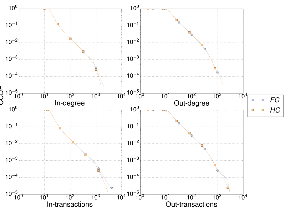
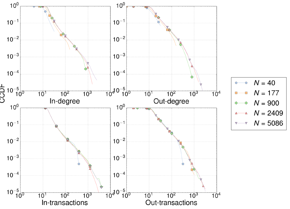
Effect of correlation. In order to study the importance of the empirical correlation observed for interbank variables (see Section 2), we constructed a number of network realizations for the correlated, random data generation schemes (FC and HC) described in Section 3.1. We did not use de NC model since it yields unrealistic interbank positions (see Table 3). Figures 7 and 8 show that both correlated methods do not condition significantly network topologies, not at least for the properties usually studied in the literature. The weak correlation between relative interbank assets (\(x\)) and liabilities (\(y\)) is only apparent in the left most part of the neighbor-averaged out-degree (Figure 8, left). These differences tend to disappear for larger networks.
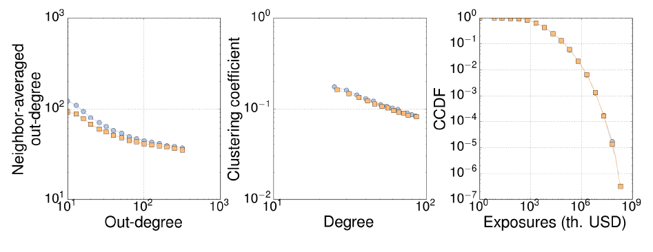
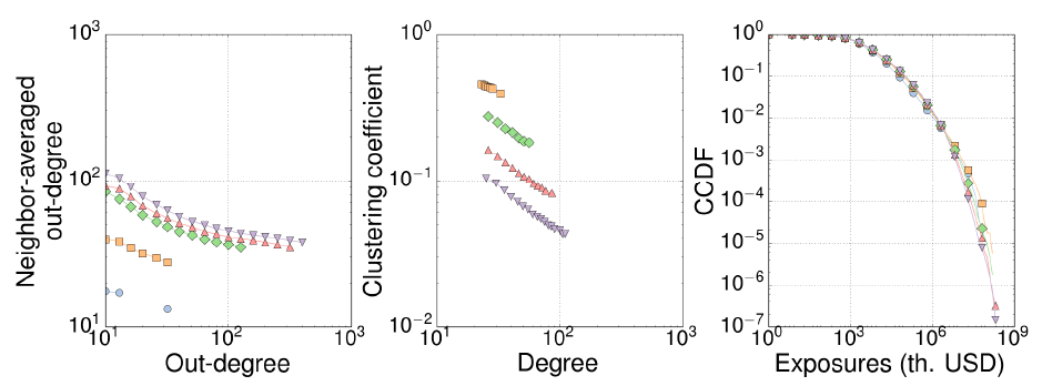
Effect of network size. All interbank networks reported in empirical works only have access to a small fraction of the total, world-wide interbank network. Our simulations in Section 4, therefore, consider network sizes that match the size of empirical networks (see Table 4). Figures 9 and 10 show that CCDF distributions (in- and out-degree, in- and out-transactions, and exposures) only differ due to a finite size effect, which appears as the cut-off of distributions. Those differences condition the average value of the out-degree and, as a consequence, assortativity (Figure 10, left) grows with network size. Clustering coefficient (Figure 10, center) decreases as network grows since the probability of creating triangles by chance also declines with network size.
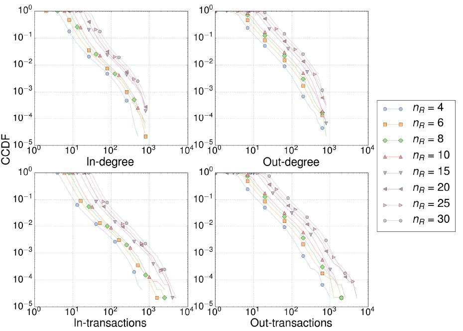
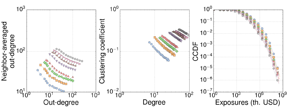
Number of rounds. Our model considers an average number of trading rounds per day, \(n_R\), which agrees with empirical observations of multiple transactions between banks within the same day (Soramäki et al. 2007). For the sake of simplicity, we assume that there is a fixed number of transactions for every bank, instead of regarding it as a random variable. As shown in Figures 11 and 12, this parameter influences all the magnitudes by increasing the number of links and the number of transactions per bank, as well as decreasing the amount of loans (exposures). It is, thus, an important parameter that deserves more attention in further improvements of the model. Additional, free-access data regarding the actual number of transactions between banks would be certainly helpful to tackle this point.
References
ACEMOGLU, D., Ozdaglar, A. & Tahbaz-Salehi, A. (2013). Systemic Risk and Stability in Networks. American Economic Review, 105(2), 564–608. [doi:10.1257/aer.20130456]
ALLEN, F., Babus, A. & Carletti, E. (2012). Asset commonality, debt maturity and systemic risk. Journal of Financial Economics, 104(3), 519–534.
ALLEN, F. & Gale, D. (2000). Financial contagion. Journal of Political Economy, 108(1), 1–33. [doi:10.1086/262109]
ASHCRAFT, A. B. & Duffie, D. (2007). Systemic illiquidity in the federal funds market. American Economic Review, 97(2), 221–225.
BASTOS e Santos, E. & Cont, R. (2010). The brazilian interbank network structure and systemic risk. Tech. Rep. 219, Banco Central do Brasil Working Paper Series.
BOSS, M., Elsinger, H., Summer, M. & Thurner, S. (2004). Network topology of the interbank market. Quantitative Finance, 4, 677–684.
CAMACHO, J., Guimerà, R. & Amaral, L. A. N. (2002). Analytical solution of a model for complex food webs. Physical Review, E 65, 030901(R). [doi:10.1103/PhysRevE.65.030901]
CAPITÁN, J. A., Arenas, A. & Guimerà, R. (2013). Degree of intervality of food webs: From body-size data to models. Journal of Theoretical Biology, 334, 35–44.
CAPITÁN, J. A., Axelsen, J. B. & Manrubia, S. (2015). New patterns in human bio-geography revealed by networks of contacts between linguistic groups. Proceedings of the Royal Society B, 282, 20142947. [doi:10.1098/rspb.2014.2947]
CAPITÁN, J. A. & Manrubia, S. (2015). Demography-based adaptive network model reproduces the spatial organization of human linguistic groups. Physical Review, E 92, 062811.
CLAUSET, A., Shalizi, C. R. & Newman, M. E. J. (2009). Power-law distributions in empirical data. Siam Review, 51(4), 661–703. [doi:10.1137/070710111]
ECB (2010). Recent advances in modelling systemic risk using network analysis. Workshop summary, European Central Bank.
FREIXAS, X., Parigi, B. M. & Rochet, J.-C. (2000). Systemic risk, interbank relations, and liquidity provision by the central bank. Journal of Money, Credit, and Banking, 32(3), 611–38. [doi:10.2307/2601198]
FRICKE, D. & Lux, T. (2015). On the distribution of links in the interbank network: evidence from the e-mid overnight money market. Empirical Economics, 49, 1467– 1495.
GAI, P. & Kapadia, S. (2010). Contagion in financial networks. Proceedings of the Royal Society of London A, 466, 2120, 2401-2423. [doi:10.1098/rspa.2009.0410]
GEORG, C.-P. (2013). The effect of the interbank network structure on contagion and common shocks. Journal of Banking & Finance, 37(7), 2216–2228.
HALDANE, A. G. & May, R. M. (2011). Systemic risk in banking ecosystems. Nature, 469(7330), 351–5. [doi:10.1038/nature09659]
IORI, G., De Masi, G., Precup, O. V., Gabbi, G. & Caldarelli, G. (2008). A network analysis of the Italian overnight money market. Journal of Economic Dynamics and Control, 32, 259–278.
IORI, G., Jafarey, S. & Padilla, F. G. (2006). Systemic risk on the interbank market. Journal of Economic Behavior & Organization, 61(4), 525–542. [doi:10.1016/j.jebo.2004.07.018]
LOEPFE, L., Cabrales, A. & Sánchez, A. (2013). Towards a proper assignment of systemic risk: The combined roles of network topology and shock characteristics. PLoS ONE , 8(10), e77526.
MARTÍNEZ-JARAMILLO, S., Alexandrova-Kabadjova, B., Bravo-Benítez, B. & Solórzano-Margain, J. P. (2012). An empirical study of the Mexican banking system’s network and its implications for systemic risk. Tech. Rep. 2012–07, Banco de México Working Papers. [doi:10.2139/ssrn.2140144]
MISHKIN, F. S. (2007). The Economics of Money, Banking, and Financial Markets. London: Pearson.
MISHKIN, F. S. (2012). Central Banking After The Crisis. Tech. Rep. November, 16 th Annual Conference of the Central Bank of Chile.http://www0.gsb.columbia.edu/faculty/fmishkin/papers/12chile.pdf.
ROHATGI, A. (2015). Webplotdigitizer: https://automeris.io/WebPlotDigitizer.
SORAMÄKI, K., Bech., M. L., Arnold, J., Glass, R. J. & Beyeler, W. L. (2007). The topology of interbank payment flows. Physica A , 379, 317–333. [doi:10.1016/j.physa.2006.11.093]
SQUARTINI, T., van Lelyveld, I. & Garlaschelli, D. (2013). Early-warning signals of topological collapse in interbank networks. Scientific reports, 3, 3357.
STOUFFER, D. B., Camacho, J. & Amaral, L. N. (2006). A robust measure of food web intervality. Proceedings of the National Academy of Sciences USA, 103, 19015–19020. [doi:10.1073/pnas.0603844103]
WILLIAMS, R. J. & Martinez, N. D. (2000). Simple rules yield complex food webs.Nature, 404, 180–183.