
Introduction
Agent-based models (ABMs) are a well-established method for the study of complex adaptive systems, in which the interactions of heterogeneous entities yield emergent large-scale behaviors. As such, this approach has been applied across a wide variety of fields such as economics, ecology, or socio-technical systems (e.g. Tesfatsion & Judd 2006; Grimm & Railsback 2012; Nikolic, Dam & Kasmire 2013).
However, the computational nature of ABMs can make them more difficult to understand and communicate than analytical models (Grimm et al. 2006). Without the use of standard frameworks to structure their analysis and documentation, ABMs may yield ad hoc, poorly reproducible results (Thiele 2015). Different initiatives are attempting to address this gap, such as the ODD and TRACE protocols for documentation (Grimm et al. 2006; Schmolke et al. 2010).
In practice, these documentation protocols are easier to apply when supported by suitable computational tools -- for instance to generate experimental designs for uncertain inputs, visualize output data, or apply standard statistical methods. While many agent-based modelling platforms include basic analysis tools, these are typically not sufficient to meet the requirements of a comprehensive analysis and documentation process. Conversely, using standalone analysis software to process input and output data files can quickly become unwieldy for complex models – making the analysis workflow more difficult to reproduce.
The literature therefore presents different connectors to directly interface agent-based modelling software with analysis environments. In particular, the popular open-source NetLogo modelling software can be linked at runtime with Mathematica (Bakshy & Wilensky 2007) and R (Thiele, Kurth & Grimm 2012), which allows modellers to use the comprehensive analysis and visualization functionalities available in these programming languages.
As a complement to these connectors, this work introduces the pyNetLogo library, which can be used to control NetLogo through the Python programming language. Python is a general-purpose language which is consistently ranked as one of the five most popular languages on the TIOBE Programming Community index (TIOBE 2017); it is increasingly used for scientific computing, and offers a variety of libraries which can support ABM development and testing. It should be emphasized that pyNetLogo is not intended as a replacement for the existing R and Mathematica connectors, or as a comment on the suitability of these various environments for ABM analysis. However, given the popularity of the Python language, pyNetLogo extends the benefits of a specialized analysis environment to a broader audience.
The following section of this paper describes the different software platforms used in this work. A software implementation section then introduces pyNetLogo and its key features, and illustrates these mechanisms for a simple predator-prey model. As an example of the analysis workflow which is enabled by pyNetLogo, this model is controlled interactively from a Python environment, then tested using a global sensitivity analysis.
Software Description
NetLogo
NetLogo (Wilensky 1999) is an open-source environment for the design and testing of agent-based models. While NetLogo was initially intended as an educational tool, its ease of use, robust performance and active user community have made it a pragmatic choice for a wide range of research applications (Kravari & Bassiliades 2015; Railsback, Lytinen & Jackson 2006). It has therefore established itself as a leading platform for agent-based modelling (Thiele 2015).
NetLogo is primarily implemented in Java and Scala, and includes a range of functions and methods to support the rapid development of spatially-explicit agent-based models. Railsback et al. (2017) further discuss strategies and techniques to improve the performance of more complex NetLogo models. In addition to connectors for Mathematica and R, different extension modules are available, for instance to interface NetLogo models with GIS datasets. In particular, an extension for Python (Head 2017) offers a converse functionality to the pyNetLogo connector, by allowing Python code to be executed from a NetLogo model.
Python
Python is a widely used high-level, general-purpose open source programming language that supports various programming paradigms. Python places a strong emphasis on code readability and code expressiveness. A large collection of libraries for many typical programming tasks is readily available. Python is increasingly popular for scientific computing purposes due to the rapidly expanding scientific computing ecosystem available for Python.
This ecosystem includes NumPy (Walt, Colbert & Varoquaux 2011) and pandas (McKinney 2010) for data manipulation, SciPy (Jones et al. 2001) for general numerical tasks, Matplotlib (Hunter 2007) for plotting and visualization, as well as Jupyter and IPython (Pérez & Granger 2007) for interactive analysis. These libraries are pre-packaged in several scientific distributions for Python, such as Continuum Anaconda. Additional libraries can be installed through standard package managers such as pip and conda.
Python is often used as a “glue” language, meaning that it connects pieces of software written in different languages together into a bigger application. For instance, the JPype library (Menard & Nell 2014) can be used to access Java class libraries through interfacing the Python interpreter and the Java Virtual Machine. PyNetLogo therefore relies on JPype for interacting with NetLogo.
Software Implementation
This section first describes basic interactions between the Python environment and a NetLogo model, using the pyNetLogo connector. These interactions are demonstrated using the simple wolf-sheep predation example which is available in NetLogo’s model library. This functionality is then extended to illustrate a typical model analysis workflow, using the SALib Python library (Herman & Usher 2017) to perform a global sensitivity analysis.
The model files used for these examples are available from the pyNetLogo repository at https://github.com/quaquel/pyNetLogo, along with interactive Jupyter notebooks which replicate the analysis and visualizations presented in this paper. Detailed documentation and installation notes for pyNetLogo are provided at http://pynetlogo.readthedocs.io. The pyNetLogo connector can be installed using the pip package manager, using the following command from a terminal or command prompt:
pip install pyNetLogo
The pyNetLogo connector has been tested with NetLogo 5.2, 5.3 and 6.0 using the 64-bit Continuum Anaconda 2.7 and 3.6 Python distributions. Using these distributions, pyNetLogo requires the additional installation of JPype (available through the conda package manager). The pyNetLogo connector is currently also included in the Exploratory Modeling Workbench Python package (Kwakkel 2017), which offers support for experiment design and exploratory modeling and analysis.
Controlling NetLogo through Python with pyNetLogo
The pyNetLogo package is composed of a Python module (core.py) and a Java JAR file (netlogolink.jar). The Python module defines a NetLogoLink class; an instance of this class is used to handle interactions on the Python side. The Python and Java environments are linked with the JPype package through the Java Native Interface (JNI). On the Java side, the JAR file provides a corresponding NetLogoLink Java class in two versions, for NetLogo 5.x and 6.0. An instance of the appropriate Java class in turn communicates with the NetLogo API. This allows for bidirectional data exchanges between a Python environment (which can for instance be an interactive Jupyter notebook) and a NetLogo model at runtime, with appropriate data type conversions between the two environments.
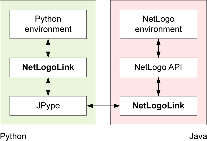
Table 1 summarizes the basic methods available through the NetLogoLink Python class. These are intended to provide “building blocks” for the interactive analysis of NetLogo models with Python, and largely replicate the basic capabilities of the RNetLogo connector for the R environment (Thiele et al. 2012). Further details are provided at http://pynetlogo.readthedocs.io.
| Name | Description | Arguments | Returns |
load_model() | Load a NetLogo model file | Model path (string) | - |
kill_workspace() | Close the NetLogo instance | - | - |
command() | Execute a given command in the NetLogo environment | Valid NetLogo command (string) | - |
report() | Return the value of a NetLogo reporter | Valid NetLogo reporter (string) | Reported value, converted to appropriate Python data type |
patch_report() | Return values for an attribute of the NetLogo patches | Valid NetLogo patch attribute (string) | pandas DataFrame of patch attribute values, with column labels and row indices following NetLogo patch coordinates |
patch_set() | Set NetLogo patch attributes from a pandas DataFrame | - Valid NetLogo patch attribute (string) - pandas DataFrame with same dimensions as the NetLogo world, containing attribute values to be set | - |
repeat_command() | Execute a given command a number of times in the NetLogo environment | - Valid NetLogo command (string) - Number of repetitions (integer) | - |
repeat_report() | Return the values of one or multiple NetLogo reporters over a given number of ticks | - Valid NetLogo reporter (string or list of strings) - Number of repetitions (integer) - NetLogo command used to execute the model (string, ‘go’ by default) | pandas DataFrame of reported values with columns for each reporter, indexed by NetLogo ticks |
write_NetLogo_attriblist() | Update a set of NetLogo agents of the same type with multiple attributes | - pandas DataFrame containing attribute values to be set, indexed by agent - Valid NetLogo agent breed (string) | - |
To illustrate the functionality of pyNetLogo, a simple example follows below, using the wolf-sheep predation model which is included in the NetLogo 6.0 example library. The Jupyter notebook available from the pyNetLogo repository replicates this example and demonstrates the key methods of the pyNetLogo connector in more detail, using a slightly modified version of the model to test a broader range of data types.
First, a link to NetLogo is instantiated. This involves starting a Java VM, followed by starting NetLogo. All interactions with NetLogo are handled by an instance of the NetLogoLink class. Note that when using Linux, the NetLogoLink class requires the netlogo_home and netlogo_version parameters to be set manually. If these parameters are not set on Mac or Windows, the class will attempt to identify and use the most recent NetLogo version found in the default program directory.
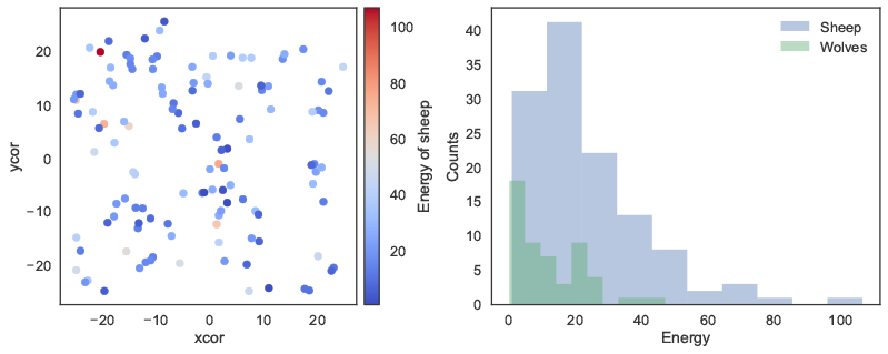
Next, we can load a model using the load_model method, followed by basic commands to set up the model and run it for 100 ticks. The report method is then used to return NumPy arrays to Python, containing the NetLogo coordinates of the "sheep" agents, and the energy attribute of the “sheep” and “wolf” agents. These arrays can then for instance be used with conventional Python functions to plot the coordinates of the agents, or the distribution of energy across agents (Figure 2).
import pyNetLogo

	netlogo = pyNetLogo.NetLogoLink(gui=True) #Show NetLogo GUI
	netlogo.load_model(r'Wolf Sheep Predation.nlogo')
	netlogo.command('setup')

	netlogo.repeat_command('go', 100)

	x = netlogo.report('map [s -> [xcor] of s] sort sheep')
	y = netlogo.report('map [s -> [ycor] of s] sort sheep')
	energy_sheep = netlogo.report('map [s -> [energy] of s] sort sheep')
	energy_wolves = netlogo.report('map [w -> [energy] of w] sort wolves')
Building on this functionality, the repeat_report method returns a pandas DataFrame containing reported values over a given number of ticks, for one or multiple NetLogo reporters. The DataFrame is structured using columns for each reporter, and indexed by NetLogo ticks. By default, this assumes the model is executed with the NetLogo go command; this command can be changed by specifying an optional go argument when calling the method.
In this case, we can first track the count of both agent types over 200 ticks. The outcomes are first plotted as a function of time on the left panel of Figure 3. On the right panel, the number of sheep agents is then plotted as a function of the number of wolf agents, to approximate a phase-space plot.
The repeat_report method can also be used with reporters that return a NetLogo list. In this case, the list will be converted into a NumPy array, which is formatted according to the data type returned by the reporter (i.e. numerical or string data).
counts = netlogo.repeat_report(['count wolves','count sheep'], 200, go='go')
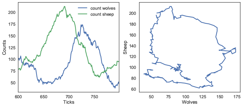
repeat_report method: number of agents as a function of time (left); number of sheep agents as a function of wolf agents (right). In addition to these reporting methods, the patch_report method can be used to return a DataFrame which contains a given patch attribute (in this case, the countdown attribute):
patch_df = netlogo.patch_report('countdown')
This DataFrame (visualized in Figure 4) essentially replicates the NetLogo environment, with column labels corresponding to the pxcor patch coordinates, row indices following the pycor coordinates, and values from the specified patch attribute. The DataFrames can be manipulated with any of the existing pandas functions, for instance by exporting to an Excel file. The patch_set method provides the inverse functionality to patch_report, and updates the NetLogo environment from a DataFrame.
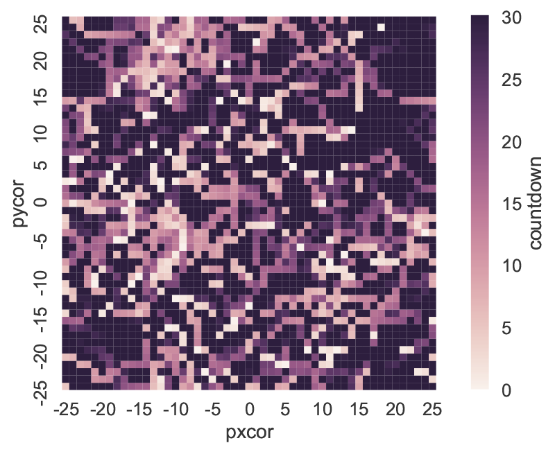
patch_report method: distribution of the countdown patch attribute across the NetLogo environment.Using Python for global sensitivity analysis on a NetLogo model
The Python environment enables access to a wide variety of packages to support the development and analysis of NetLogo models. As an example, this subsection uses the SALib Python library for a global sensitivity analysis (GSA) on the wolf-sheep predation model presented earlier. The full code used for the analysis and visualizations can be found in the Jupyter notebook available from the pyNetLogo repository.
By contrast to “one-at-a-time” sensitivity analysis, which evaluates the response of a model to changes in individual parameters, GSA aims to capture the behavior of the model across the full domain of uncertain inputs (see e.g. Saltelli et al. 2008 for a comprehensive overview). This is especially useful for models in which interactions between parameters can be expected to be significant. A simple example of GSA would be generating a Monte Carlo sample of all uncertain inputs, then applying a multiple linear regression to the model output.
For more complex, non-linear models, variance-based approaches such as Sobol indices (Sobol 1993) can accurately capture each parameter’s contribution to the variance of model output. Sobol indices are computed using variance decomposition; first-order and total indices respectively estimate the fractional contribution of each input to output variance on its own, and inclusive of interactions with other inputs. Second-order indices can also be computed to estimate the contribution of pairwise variable interactions towards output variance. However, this type of variance-based analysis requires specific techniques for input sampling and output analysis.
In this context, the SALib library provides sampling and analysis modules for methods including Sobol indices, Morris elementary effects (Campolongo, Cariboni & Saltelli 2007; Morris 1991), and derivative-based global sensitivity measures (Sobol’ & Kucherenko, 2009). Integrating these methods within a NetLogo workflow significantly extends the functionality of NetLogo’s BehaviorSpace tool, which has limited sampling options. This example will use SALib to estimate Sobol indices; although these indices accurately represent input importance, their calculation may require a large input sample size to yield stable results. For complex models which may be too time-consuming to simulate over such an ensemble of experiments, the Morris elementary effects technique can instead be used from SALib to “screen” non-influential variables at a smaller sample size, while still accounting for parameter interactions and non-linearities which may be missed by a “one-at-a-time” approach. Ayllón et al. (2016) describe an application of this method for a complex NetLogo model.
SALib relies on a problem definition dictionary (i.e., a key-value map), which contains the number of input parameters to sample, their names (which should here correspond to a NetLogo global variable), and the sampling bounds:
	problem = {
		'num_vars': 6,
		'names': ['random-seed','grass-regrowth-time','sheep-gain-from-food',
				  'wolf-gain-from-food','sheep-reproduce','wolf-reproduce'],
		'bounds': [[1, 100000], [20., 40.], [2., 8.],
					[16., 32.], [2., 8.], [2., 8.]]
	}
The SALib sampler will then generate an appropriate experimental design based on the analysis technique to be used. To calculate first-order, second-order and total Sobol sensitivity indices, this gives a sample size of n(2p+2), where p is the number of input parameters, and n is a baseline sample size which should be large enough to stabilize the estimation of the indices.
For this example, we use n = 1000, for a total of 14000 experiments. The next subsection will demonstrate the use of ipyparallel to parallelize the simulations and reduce runtime.
from SALib.sample import saltelli
	from SALib.analyze import sobol

	n = 1000
	# Generates an input array of shape (n*(2p+2), p) with rows for each
	# experiment and columns for each input
	param_values = saltelli.sample(problem, n, calc_second_order=True)
Assuming we are interested in the mean number of sheep and wolf agents over a timeframe of 100 ticks, we first create an empty DataFrame to store the results. We then simulate the model over the 14000 experiments, by reading input parameters from the param_values array generated by SALib and using the repeat_report method to track the outcomes of interest over time.
	results = pd.DataFrame(columns=['Avg. sheep', 'Avg. wolves'])

	for run in range(param_values.shape[0]):
		# Set the input parameters
		for i, name in enumerate(problem['names']):
			if name == 'random-seed':
				# The NetLogo random seed requires a different syntax
				netlogo.command('random-seed {}'.format(param_values[run,i]))
			else:
				# Otherwise, assume the input parameters are global variables
				netlogo.command('set {0} {1}'.format(name, param_values[run,i]))

    netlogo.command('setup')
		# Run for 100 ticks and return the number of sheep and wolf agents at
		# each time step
		counts = netlogo.repeat_report(['count sheep','count wolves'], 100)

		# For each run, save the mean value of the agent counts over time
		results.loc[run, 'Avg. sheep'] = counts['count sheep'].values.mean()
		results.loc[run, 'Avg. wolves'] = counts['count wolves'].values.mean()
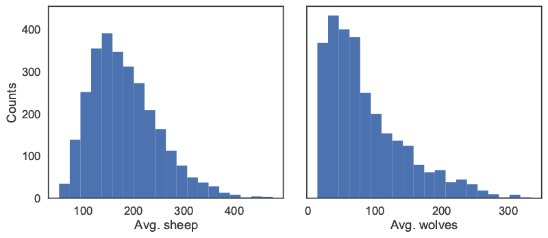
We can then proceed with the analysis, first using a histogram to visualize output distributions for each outcome as shown in Figure 5.
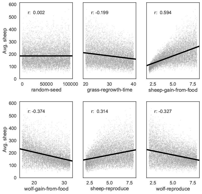
Bivariate scatter plots can be useful to visualize relationships between each input parameter and the outputs. Taking the outcome for the average sheep count as an example, we obtain Figure 6, using SciPy to calculate the Pearson correlation coefficient (r) for each parameter. This indicates a positive correlation between the sheep-gain-from-food parameter and the mean sheep count, and negative correlations for the wolf-gain-from-food and wolf-reproduce parameters.
We can use SALib to calculate first-order (S1), second-order (S2) and total (ST) Sobol indices, to estimate each input's contribution to the variance of the average sheep count. By default, 95% confidence intervals are also estimated for each index. The analysis function returns a Python dictionary.
Si = sobol.analyze(problem, results['Avg. sheep'].values, calc_second_order=True)
As a simple example, Figure 7 visualizes the first-order and total indices and their confidence bounds (shown as error bars) using the default pandas plotting functions, after converting the dictionary returned by SALib to a DataFrame:
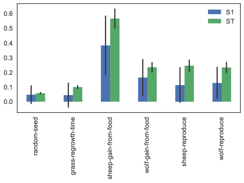
The sheep-gain-from-food parameter has the highest S1 and ST indices, indicating that it contributes roughly 40% of output variance on its own, and over 50% when accounting for interactions with other parameters. However, the first-order confidence bounds are overly broad due to the relatively small n value used for sampling (i.e. 1000), so that a larger sample would be required for reliable results.
We can use a more sophisticated visualization to include the second-order pairwise interactions between inputs, shown in Figure 8. The size of the ST and S1 circles correspond to the normalized total and first-order indices, and the width of connecting lines between variables indicates the relative importance of their pairwise interactions on output variance.
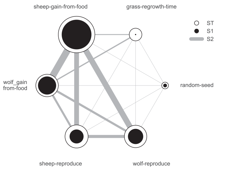
In this case, the sheep-gain-from-food variable has strong interactions with the wolf-gain-from-food and wolf-reproduce inputs in particular, as indicated by their thicker connecting lines.
Using ipyparallel for parallel simulation
ipyparallel is a standalone package (available through the conda package manager) which can be used to interactively run parallel tasks from IPython on a single PC, but also on multiple computers. On machines with multiple cores, this can significantly improve performance: for instance, the multiple simulations required for a sensitivity analysis are easy to run in parallel. This subsection will repeat the global sensitivity analysis presented in the previous subsection, this time using ipyparallel to distribute the simulations across multiple cores on a single computer. The code fragments assume the analysis is executed from a Jupyter notebook; as with the previous examples, the full notebook is available from the pyNetLogo repository.
ipyparallel first requires starting a controller and multiple engines, which can be done from a terminal or command prompt with the following:
ipcluster start -n 4
The optional -n argument specifies the number of processes to start (4 in this case). By default, the number of logical processor cores will be used.
Next, we can connect the interactive notebook to the cluster by instantiating a client (within a notebook), and checking that client.ids returns a list of 4 available engines.
import ipyparallel

	client = ipyparallel.Client()
	print(client.ids)
After defining the SALib problem dictionary and input sample as in the previous subsection, we can then set up the engines so that they can run the simulations, using a "direct view" that accesses all engines. We first need to ensure the engines can access the current working directory in order to find the NetLogo model. We can then also pass the SALib problem definition dictionary to the engines.
direct_view = client[:]
	import os

	# Push the current working directory of the notebook to a
	# "cwd" variable on the engines that can be accessed later
	direct_view.push(dict(cwd=os.getcwd()))

	# Push the "problem" variable from the notebook to a
	# corresponding variable on the engines
	direct_view.push(dict(problem=problem))
The %%px command can be added to a notebook cell to run it in parallel on each of the engines. Here the code first involves some imports and a change of the working directory. We then start a link to NetLogo, and load the example model (assumed to be in the working directory) on each of the engines.
%%px

	import os
	os.chdir(cwd)

	import pyNetLogo
	import pandas as pd

	netlogo = pyNetLogo.NetLogoLink(gui=False)
	netlogo.load_model(r'Wolf Sheep Predation_v6.nlogo')
We can then use ipyparallel’s map functionality to run the sampled experiments, now using a "load balanced" view to automatically handle the scheduling and distribution of the simulations across the engines. This is useful when simulations may take different amounts of time.
We first slightly modify the simulation code used previously, setting up a simulation function that takes a single experiment (i.e. a vector of input parameters) as an argument, and returns the outcomes of interest in a pandas Series.
	def run_simulation(experiment):

		# Set the input parameters
		for i, name in enumerate(problem['names']):
			if name == 'random-seed':
				# The NetLogo random seed requires a different syntax
				netlogo.command('random-seed {}'.format(experiment[i]))
			else:
				# Otherwise, assume the input parameters are global variables
				netlogo.command('set {0} {1}'.format(name, experiment[i]))

		netlogo.command('setup')
		# Run for 100 ticks and return the number of sheep and wolf agents at each time
		# step
		counts = netlogo.repeat_report(['count sheep','count wolves'], 100)

		results = pd.Series([counts['count sheep'].values.mean(),
                             counts['count wolves'].values.mean()],
                            index=['Avg. sheep', 'Avg. wolves'])

		return results
We then create a load balanced view, and run the simulation with the view’s map_sync() method. This method takes a function and a Python sequence as arguments, applies the function to each element of the sequence, and returns results once all computations are finished. In this case, we pass the simulation function and the array of experiments (param_values), so that the function will be executed for each row of the array.
The DataFrame constructor is used to immediately build a DataFrame from the results (which are returned as a list of Series).
	lview = client.load_balanced_view()
	results = pd.DataFrame(lview.map_sync(simulation, param_values))
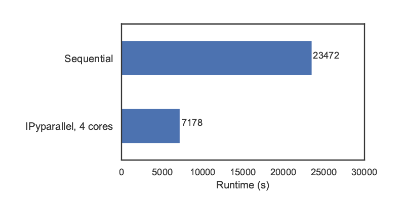
We can then proceed with the analysis as in the previous subsection. Figure 9 compares the runtimes obtained with ipyparallel and a sequential simulation (using an Intel i7-6700HQ CPU) for 14000 experiments. The elapsed parallel runtime is approximately one-third of the sequential runtime; given that we were using 4 engines, this is slightly more than could be expected from a perfectly parallel computation, due to the overhead involved in data exchanges, etc.
Conclusions
The analysis and communication of agent-based models can benefit from the comprehensive analysis features which are available in specialized software environments. To this end, this paper first introduced the pyNetLogo connector, which interfaces the NetLogo agent-based modelling software with a Python environment. This connector provides basic command and reporting functionalities similar to the RNetLogo package in R. These features were illustrated using one of NetLogo’s sample models. As an example of the more complex analyses which are enabled by a Python interface, the SALib Python library was then used for a Sobol variance-based global sensitivity analysis of the model. This analysis was performed using sequential simulations, then parallelized for improved performance using the ipyparallel library.
The current implementation of pyNetLogo relies on a Java Native Interface (JNI) through the JPype library, which allows Java classes (and thus NetLogo) to be called from Python. However, this does not support a bidirectional linkage through which a NetLogo model could also directly execute Python code. For applications in which this functionality would be helpful (for instance by using more advanced statistical or geospatial functions in NetLogo models), the Python extension for NetLogo can instead be used to execute Python code from NetLogo through a JSON interface. As a complement to existing interfaces which link NetLogo with R or Mathematica, the combination of these tools thus allows modellers to extend NetLogo’s capabilities with Python’s extensive ecosystem for scientific computing.
Acknowledgements
This research was supported by the Netherlands Organization for Scientific Research (NWO) under the project Aquifer Thermal Energy Storage Smart Grids (ATES-SG), grant number 408-13-030. We thank two anonymous reviewers for their valuable comments that helped us improving the paper.References
AYLLÓN, D., Railsback, S. F., Vincenzi, S., Groeneveld, J., Almodóvar, A., & Grimm, V. (2016). InSTREAM-Gen: Modelling eco-evolutionary dynamics of trout populations under anthropogenic environmental change. Ecological Modelling, 326(Supplement C), 36–53. [doi:10.1016/j.ecolmodel.2015.07.026]
BAKSHY, E., & Wilensky, U. (2007). NetLogo-Mathematica Link. Center for Connected Learning and Computer-Based Modeling, Northwestern University, Evanston, IL. Retrieved from http://ccl.northwestern.edu/netlogo/mathematica.html.
CAMPOLONGO, F., Cariboni, J., & Saltelli, A. (2007). An effective screening design for sensitivity analysis of large models. Environmental Modelling & Software, 22(10), 1509–1518. [doi:10.1016/j.envsoft.2006.10.004]
GRIMM, V., Berger, U., Bastiansen, F., Eliassen, S., Ginot, V., Giske, J., Goss-Custard, J., Grand, T., Heinz, S.K., Huse, G., Huth, A., Jepsen, J.U., Jørgensen, C., Mooij, W.M., Müller, B., Pe'er, G., Piou, C., Railsback, S.F., Robbins, A.M., Robbins, M.M., Rossmanith, E., Rüger, N., Strand, E., Souissi, S., Stillman, R.A., Vabø, R., Visser, U. and DeAngelis, D.L. (2006). A standard protocol for describing individual-based and agent-based models. Ecological Modeling, 198, 115-126. [doi:10.1016/j.ecolmodel.2006.04.023].
GRIMM, V., & Railsback, S. F. (2012). Pattern-oriented modelling: a "multi-scope" for predictive systems ecology. Philosophical Transactions of the Royal Society of London B: Biological Sciences, 367(1586), 298–310. [doi:10.1098/rstb.2011.0180]
HEAD, B. (2017). NetLogo Python extension. Retrieved from https://github.com/qiemem/PythonExtension.
HERMAN, J., & Usher, W. (2017). SALib: An open-source Python library for Sensitivity Analysis. The Journal of Open Source Software, 2(9). [doi:10.21105/joss.00097]
HUNTER, J. D. (2007). Matplotlib: A 2D Graphics Environment. Computing in Science & Engineering, 9(3), 90–95.
JONES, E., Oliphant, T., Peterson, P., & others. (2001). SciPy: Open source scientific tools for Python. Retrieved from http://www.scipy.org/.
KRAVARI, K., & Bassiliades, N. (2015). A Survey of Agent Platforms. Journal of Artificial Societies and Social Simulation, 18(1), 11: https://www.jasss.org/18/1/11.html.
KWAKKEL, J. H. (2017). The Exploratory Modeling Workbench: An open source toolkit for exploratory modeling, scenario discovery, and (multi-objective) robust decision making. Environmental Modelling & Software, 96, 239–250. [doi:10.1016/j.envsoft.2017.06.054]
MCKINNEY, W. (2010). Data Structures for Statistical Computing in Python. In Stéfan van der Walt & J. Millman (Eds.), Proceedings of the 9th Python in Science Conference (pp. 51–56).
MENARD, S., & Nell, L. (2014). Jpype. Retrieved from https://pypi.python.org/pypi/JPype1.
MORRIS, M. D. (1991). Factorial Sampling Plans for Preliminary Computational Experiments. Technometrics, 33(2), 161–174.
NIKOLIC, I., Dam, K. H. van, & Kasmire, J. (2013). 'Practice.' In K. H. van Dam, I. Nikolic, & Z. Lukszo (Eds.), Agent-Based Modelling of Socio-Technical Systems (pp. 73–137). Dordrecht: Springer Netherlands. [doi:10.1007/978-94-007-4933-7_3]
PÉREZ, F., & Granger, B. E. (2007). IPython: A System for Interactive Scientific Computing. Computing in Science & Engineering, 9(3), 21–29.
RAILSBACK, S., Ayllón, D., Berger, U., Grimm, V., Lytinen, S., Sheppard, C., & Thiele, J. (2017). Improving Execution Speed of Models Implemented in NetLogo. Journal of Artificial Societies and Social Simulation, 20(1), 3: https://www.jasss.org/20/1/3.html [doi:10.18564/jasss.3282]
RAILSBACK, S., Lytinen, S., & Jackson, S. (2006). Agent-based Simulation Platforms: Review and Development Recommendations. Simulation, 82(9), 609–623.
SALTELLI, A., Ratto, M., Andres, T., Campolongo, F., Cariboni, J., Gatelli, D., Saisana, M & Tarantola, S. (2008). Global sensitivity analysis: The primer. Chichester: John Wiley & Sons.
SCHMOLKE, A., Thorbek, P., DeAngelis, D. L., & Grimm, V. (2010). Ecological models supporting environmental decision making: a strategy for the future. Trends in Ecology & Evolution, 25(8), 479–486.
SOBOL, I. M. (1993). Sensitivity estimates for nonlinear mathematical models. Mathematical Modelling and Computational Experiments, 1(4), 407–414.
SOBOL’, I. M., & Kucherenko, S. (2009). Derivative based global sensitivity measures and their link with global sensitivity indices. Mathematics and Computers in Simulation, 79(10), 3009–3017.
TESFATSION, L., & Judd, K. L. (2006). 'Preface.' In L. T. and K. L. Judd (Ed.), Handbook of Computational Economics (Vol. 2, pp. xi–xv). North Holland: Elsevier. [doi:10.1016/S1574-0021(05)02039-3]
THIELE, J. C. (2015). Towards Rigorous Agent-Based Modelling (Doctoral dissertation). Georg-August-Universität Göttingen, Göttingen. Retrieved from https://ediss.uni-goettingen.de/handle/11858/00-1735-0000-0023-997B-8.
THIELE, J. C., Kurth, W., & Grimm, V. (2012). Agent-Based Modelling: Tools for Linking NetLogo and R. Journal of Artificial Societies and Social Simulation, 15(3), 8: https://www.jasss.org/15/3/8.html. [doi:10.18564/jasss.2018]
TIOBE. (2017). TIOBE Programming Community index. Retrieved from https://www.tiobe.com/tiobe-index/.
WALT, S. van der, Colbert, S. C., & Varoquaux, G. (2011). The NumPy Array: A Structure for Efficient Numerical Computation. Computing in Science Engineering, 13(2), 22–30. [doi:10.1109/MCSE.2011.37]
WILENSKY, U. (1999). NetLogo (Version 5.1.0). Center for Connected Learning and Computer-Based Modeling, Northwestern University.