Identifying Mechanisms Underlying Peer Effects on Multiplex Networks

Introduction

Social scientists have long been interested in understanding the influence of social interactions on economic behaviours. One area that has been intensively studied is peer effects in the diffusion of innovations (Rogers 2003). Peer effects have been found in people's adoption of innovations in many fields including agriculture (e.g., Ryan & Gross 1943; Rogers 1970; Munshi 2004; Conley & Udry 2010), health (e.g., Coleman et al. 1966; Rogers & Kincaid 1981; Valente & Saba 1998; Christakis & Fowler 2007) and finance (e.g., Banerjee et al. 2013; Bursztyn et al. 2014). Recent literature shows increasing interest in investigating how peer effects occur, rather than simply whether peer effects occur overall, by looking into the underlying mechanisms through which peer effects take place. A significant body of studies focuses on social learning (e.g., Munshi 2004; Bandiera & Rasul 2006; Conley & Udry 2010; Genius et al. 2014), in which "learning" is broadly defined as the uptake of new information (Foster & Rosenzweig 2010). The information can be the awareness about the existence of the innovation or the knowledge about the feasibility or profitability of the innovation. These different types of information often transmit through different channels and can play different roles in shaping a diffusion process. For example, Banerjee et al. (2013) find the transmission of awareness information has a significant influence on farmers' decisions to take up micro-credit, but the interactions with regard to other types of information do not. Another body of literature examines the role of externalities, showing peers' adoption behaviour can positively or negatively affect individuals' payoff from current choice and thus discourage or motivate the individuals to adopt (e.g., Abdulai & Hu man 2005; den Broeck & Dercon 2011). Behaviours, unlike information or disease, spread as complex contagions (Centola & Macy 2007), meaning that it requires multiple sources of reinforcement to induce peoples' adoption. Therefore, peer effects in the diffusion of innovations often take place through multiple channels. In this study, we test the causal effects of two channels, i.e., social learning and externalities, on driving farmers' adoption of a new crop.

Identifying peer effects through different channels is a challenging task. First, the traditional selection and reflection problems exist. The selection problem refers to the bias that peer groups are formed endogenously due to the similarities across individuals (Manski 1993; Goette et al. 2012). The reflection problem characterises the challenge that the pure peer effects could be mingled with the influences of other factors, e.g., interdependent personal characteristics and common shocks, that could give rise to similar observed outcomes (Manski 1993; Bramoulle et al. 2009; Goldsmith-Pinkham & Imbens 2013). In addition, the effects driven through different channels could intertwine in the diffusion process, reinforcing or offsetting each other (Dahl et al. 2014). For instance, at the same time as some farmers are informed about a new crop, those who have adopted could be sharing the experiential know-how of farming the crop. The externalities that force the non-adopters not to adopt could take place at one hand, while the tacit knowledge that helps reduce the cost to adopt is spread on the other hand.

The context we study is the diffusion of a crop called Artemisia slengensis (AS) in the rural villages located in central China. AS was newly introduced into 10 villages in 2001 and had been adopted by all households by 2009. With a survey of the population of 463 households in these 10 villages, we are able to identify the three major types of relationships, namely, kinship, house neighbourhood and land plot neighbourhood (Xiong & Payne 2017), in each village. The village census also collects each household's adoption year. Using the naturally occurring relationships, rather than acquired relationships such as friendship, immunises our estimation of peer effects to the selection problem^[1]. In addition, we conduct our estimation in each year of the entire diffusion process. Correlated unobservables are thus less likely to bias our estimation.

Both social learning and externalities played an important role in the process that the adoption of the new crop diffused. Social learning took place as farmers shared seed-stalks of AS as well as planting techniques and market information from the earlier adopters. These resources were scarce and of great value at the time. They were shared only between family members and house neighbours (often also members of the extended family). Externalities were observed between neighbouring land plots belonging to different farmers. Farming AS required much more water than farming the traditional crop (i.e., cotton), and the water in the AS plots could flow or penetrate into the adjacent cotton plot and cause damage. Cotton farmers neighbouring many AS plots were therefore forced to follow suit.

We develop an agent-based model to represent the effects of social learning and externalities on a multiplex network with two layers, each hosting a dynamic process (Xiong et al. (2018) present a theoretical application of this model). Peer effects through the two channels are tested both separately and jointly, and at different phases of the diffusion process. We find evidence for effects through both channels. The effect of social learning is significant over the entire diffusion process and plays a dominant role in the early phase, whereas externalities only matters in the late phase. These findings are robust to the estimations conducted by fitting the model to different subgroups of the population and by considering the inter-village effect.

Background and Data

Background

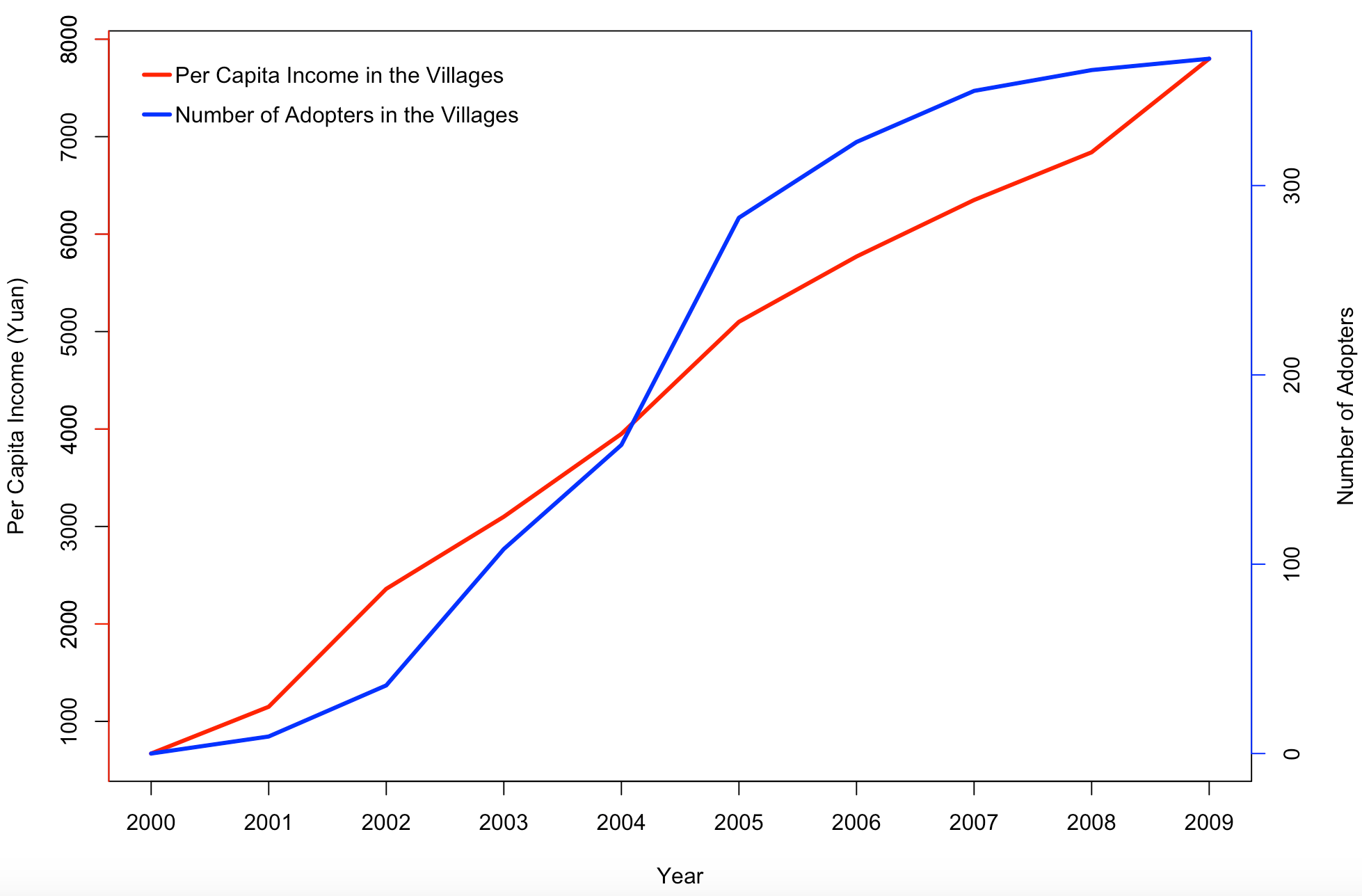
We study 10 villages located in the rural area of Wuhan, a city in central China. The farmers in these villages traditionally farmed paddy rice and cotton. To increase farmers' income, the local county government introduced a high-value vegetable into nearly 100 villages in early 2001. The new vegetable, as seed-stalks, was imported from a city 2,000 km away and was distributed to all households in these villages. As most of the farmers did not believe farming this vegetable could make profit, only about 20 households in the 10 villages planted AS in the first year. However, it turned out farming AS was several times more profitable than farming traditional crops, which encouraged other farmers to follow suit. The earliest adopters then became the only sources of seed-stalks, which were saved from last year's harvest. By 2005, more than 60% of the households in most of these 10 villages had adopted the new crop. By 2009, all households that could potentially adopt the new crop in these villages had adopted. As a result, the per capita income in these villages soared from less than 700 RMB in 2000 to nearly 8,000 RMB in 2009. Figure 1 presents the adoption rates and the income growth over all the villages from 2001 to 2009.

By 2010, the new crop was not being grown in any village apart from the 10 with adopters in the first year. This was because the stalk-seeds had not been reserved in other villages (the initially distributed stalk-seed could stay alive for about merely 10 days), whereas the growers kept the seed-stalks within their own villages. This study focuses on the diffusion in 10 villages before 2010. The diffusion in these villages took place independently, despite the fact that the villages are geographically quite close. This was possible because land was collectively owned at the village level (even the per capita farmland varies significantly among these villages, from fewer than 1 mu^[2] to over 5 mu) and the infrastructure, including irrigation systems and roads, was owned and managed independently by these villages.

Data

Detailed data were collected from the studied villages. They include the data indicating when each farm adopted AS (diffusion data), the data of different types of social ties (network data) and those characterising the household level socioeconomic states (demographic data). The dataset containing these data is publicly available at Xiong et al. (2016b).

Diffusion data

We conducted questionnaire surveys over all households in each village. In the questionnaire, farmers were asked the years in which they started to farm AS and the acreage they farmed since then. The survey results were checked against two pieces of documentary evidence. One was the historical imagery in the Google Earth map, from which land plots on which AS grew in 2003 can be identified. The other were the records of AS growers from 2004 to 2007 that were made for conducting a government program that subsided vegetable growers. When there was a contradiction, we returned to the relevant respondent for clarification or correction.

Network data

Kinship and neighbourhood are the most important social relationships in rural China (Xiong & Payne 2017). Detailed data of each farm's kinship ties, house and land plot neighbourhood ties were collected. Kinship consists of blood relationship (based on genes) and affinity relationship (based on marriage). The blood relationship between households (represented by that of heads of household) is documented in the form of family trees of the lineage they belong to. There are a total of 63 lineages in the 10 villages (it is often that a whole lineage was in one village). We collected the family trees of all the lineages. We also collected the information of marriages, where both the husband and wife are in the surveyed villages, that took place in the period from 1950 to 2000. We then calculated the weights of blood relationships according to the closeness in blood, namely, the degree of consanguinity and the weights of affinity relations according to the weights of blood relations of members that a marriage involves (the methods are elaborated in Xiong et al. 2016c).

The data of house neighbourhoods were collected using Google Earth maps, on which all houses in these villages can be clearly marked. We then used a GIS tool (ArcGIS) to identify neighbourhoods between the houses. Two houses fewer than 15 meters (roughly the width of a house in regular size plus the width of the narrow gap between two houses) apart are viewed as the first degree neighbour to each other, and the weight of the neighbourhood is set to be 1. Likewise, the distance between 15 to 30 meters indicates second degree neighbourhood and its weight is set to be 0.5.

The farmland of a village is split into many small-size plots. The acreage of a plot ranges from 0.1 mu to more than 2 mu and a household could have 5-8 plots that were often not adjacent to each other. Each plot's neighbouring plots in four orientations are clearly listed in the land contract that the household signed with the village committee. To reflect the feature that smaller plots have less influence on households' production decisions than larger ones, we categorised the land plots into small, medium and large sizes according to their acreage, and assigned the ties linking to plots in each category a different weight in the network. Specifically, a plot smaller than 0.50 mu is a small plot, larger than 0.51 and smaller than 1.00 mu is a medium one, and larger than 1.01 mu is a large one. Accordingly, the weights of ties linking to plots in each category are 1/4, 1/2 and 1, respectively.

All these social relationship existed before the diffusion of AS and they were almost constant during the process of diffusion. This thus immunises our identification of peer effects to the self-selection problem.

Demographic data

We also obtained comprehensive household level demographic data covering acreage of land and number of farming workers of households, surnames (used for identify lineages), year of birth and number of schooling years of the heads of household, in each village from 2000 to 2014.

Observation selection

Our observations in each village are selected as the following procedure. We began with the list of the households that signed a land contract (because this is a board list). There are a total of 463 households on the list over all villages. To select the households that have the conditions of farming AS, we then excluded the following households from the list: (i) Those with all farming workers had retired before 2000; (ii) non-independent households (such as the divorced, orphans, persons serving prison sentences, etc.); (iii) households that have emigrated from their villages^[3] before 2000; (vi) households moved away after 2000 and had not adopted before they gave up farming; (v) households with no or limited ability to practise farming (such as the disabled, the aged, widows or widowers without close offspring in the village, etc.); and (vi) households doing non-farming jobs (such as running a convenience shop, operating a small restaurant, bricklayers and rag pickers, etc.). Finally, 367 households, accounting for about 80% of the original list, were remained. The details of the selection process are displayed in Table 1.

Table 1: Selection of Household Observations

	1	2	3	4	5	6	7	8	9	10	Total	Percentage
Households Signing Land Contracts	50	57	35	31	61	67	59	19	57	27	463	100.00%
Non-farming Parent(s) Households	0	3	5	4	5	3	4	1	0	2	27	5.83%
Non-independent Households	1	0	2	0	0	2	2	0	1	2	10	2.16%
Households Emigrating before 2000	5	2	1	1	4	1	0	0	1	1	16	3.46%
Emigrating after 2000 and Non-adopting	1	1	2	1	3	2	2	1	2	0	15	3.24%
Households Lack of Labour	0	4	0	1	5	3	6	0	3	1	23	4.97%
Non-farming Households	1	1	1	0	0	0	2	0	0	0	5	1.08%
Households Capable of Adopting	42	46	24	24	44	56	43	17	50	21	367	79.27%

Definition of adoption

This study takes a household that farms AS for no fewer than 1 mu as an adopter ^[4] and accordingly the year in which the acreage of AS farming first reached 1 mu as the year a household adopted. This definition helps separate actual adoption from trial adoption. Among the observed households, we found no household gave up once they had adopted^[5]. This was the case because farming AS was evidently much more profitable than farming other crops. Also, it is more attractive than working in cities from the perspective that farmers can better look after their families. In our study, therefore, we reasonably assume a household keeps adopting once it has started.

Descriptive statistics

Table 2 present the statistical characteristics of the households and the social networks in which are embedded. The villages we study have an average of 37 households, with a cross-village standard deviation of 14. There are nearly 8 lineages in a village on average, but the number is quite diverse (varying from 3 to 13). A lineage has, on average, 7 households, also with large variance (the standard deviation is 4.6 across lineages). The average age of heads of household is 42 year-old in 2000 and the cross-village variation is small (fewer than 3 years). Most heads of household have completed the education in the junior middle school, i.e., 9 years' schooling. Those who have education higher or lower than this level are both rare. There are averagely about 2.3 labours in a household, with the standard deviation of 0.5 across villages. The acreage of land a typical household has is about 5 mu. In general, these results show that the villages are small but there are potentially dense connections via kinship within a village. Households are quite homogeneous in terms of the age of head, education and labour.

We measured the network characteristics of the villages based on the networks consisting of the kinship and house neighbourhood ties, the land plot neighbourhood ties and the ties of all the three relationships. The three types of networks are chosen because we will estimate peer effects based on them. The kinship ties and house neighbourhood ties in the networks are combined together because they are highly overlapped in the villages (Xiong & Payne 2017). The results show that the kinship and house neighbourhood networks are densely connected (the average degree, strength and density are high) and completely clustered (clustering coefficient is 1; obviously in the unit of lineage). However, the distance (indicated by average path length and diameter) between the households are high, implying that there are few linkages between clusters. Furthermore, the high degree centralisation suggests there are opinion leader type individuals in lineages. On the contrary, the land plot neighbourhood networks are less connected and clustered but the distance between households are much shorter. The results of the whole networks (i.e., combined kinship, house neighbourhood and land plot neighbourhood networks) generally fall between those of kinship and house neighbourhood networks and those of land plot neighbourhood networks. Overall, these results suggest that kinship and house neighbourhood networks can facilitate the diffusion of innovations within clusters, each of which possibly contains opinion leaders. Land plot neighbourhood networks, on the other hand, can help the spreading between clusters.

Table 2: Descriptive statistics of networks and households characteristics

	Mean	Standard Deviation	Maximum	Minimum
Panel A: Demographic Characteristics
Number of Households (Nodes in networks)	36.70	13.80	18	67
Number of Lineage	7.60	5.21	3	14
Number of Households per Lineage	6.61	4.65	4	20.67
Average Age	42.13	2.70	47.29	39.83
Average Education Level	1.96	0.20	2.25	1.61
Average Amount of Labour	2.31	0.51	3.53	1.95
Average Land per Household (mu)	5.00	0.67	5.84	3.53
Panel B: Networks Characteristics
Kinship + House Neighbourhood Networks
Average Degree (average number of ties)	21.98	11.93	45.61	6.78
Strength (number of ties considering weights)	3.66	0.90	4.94	1.72
Density (chance of a tie exists between nodes)	0.55	0.24	1.00	0.24
Clustering Coefficient (chance of mutual ties)	1.00	0.00	1.00	1.00
Average Path Length	4.47	2.12	10.02	2.49
Diameter (maxima path length)	7.05	2.73	13.28	4.57
Centralisation (concentration or inequality)	0.70	0.15	0.93	0.41
Land Plot Neighbourhood Networks
Average Degree	8.65	s	14.37	5.68
Strength	2.33	1.11	4.78	1.26
Density	0.24	0.13	0.59	0.10
Clustering Coefficient	0.35	0.11	0.64	0.21
Average Path Length	2.16	0.58	3.30	1.27
Diameter	5.98	2.44	9.62	2.51
Centralisation	0.73	0.13	0.92	0.52
Whole Networks
Average Degree	26.67	9.95	48.58	13.11
Strength	6.25	0.98	8.23	4.71
Density	0.65	0.19	1.00	0.42
Clustering Coefficient	0.82	0.13	1.00	0.65
Average Path Length	1.04	0.22	1.36	0.74
Diameter	2.15	0.45	2.85	1.46
Centralisation	0.54	0.14	0.84	0.36
Panel C: Other Characteristics
Average Distance to Arterial Road (km)	8.45	2.95	11.50	5.55

Mechanisms underlying peer effects

In our case, all the households were informed about the new crop by their village leaders on the first day it was introduced into the villages. The spread of the information about the existence of the innovation thus, if existed, would have very limited influence on motivating a farmer to adopt. Farmers in these villages, due to their low capacity to bear any significant loss, generally would not adopt a new crop before they were convinced about its profitability (e.g., being shown the price and production is higher than those of traditional crops). This is confirmed by the fact that fewer than 20 out of the 376 households tried to plant the new crop in the first year, even though seed-stalks were freely given to them. For these reasons, we do not think the transmission of awareness of the crop is an important factor influencing the diffusion process. In our model, the adopters in the first two years are set as seed adopters.

Social learning

Social learning could take place through channels that earlier adopters could share their planting techniques, market information or seed-stalks with the potential adopters. The techniques of managing water and applying fertiliser and pesticide in farming AS is quite different from those used in farming rice and cotton. These specific techniques were tacit knowledge and could only be obtained by participating in person or learning from earlier practitioners. Similarly, the market information about the specific crop was limit and farmers could only obtain it from their fellows who had experience of selling AS. Accessibility to tacit techniques or market information from earlier adopters, therefore, could increase one's propensity to adopt. Here we draw a distinction between adoption in decision and adoption in action, which is rarely considered in the literature as decision and action often occur simultaneously. In our case, even if a farmer had decided to adopt, he might not be able to actually do so, due to the inaccessibility of seed-stalks, and the season when the decision to adopt took place. If one did not farm AS when it was first introduced, the only feasible source to obtain the seed-stalks was from the adopters after the first year, because (i) it was not possible to obtain the seed-stalks from the original place where the AS stalks were brought from (an city which is about 2,000 km away) or other nearby places, (ii) the seed-stalks were not sold in market, and (iii) there was no substitute for that variety of AS.

In the first few years, when growers were rare, the opportunity cost of saving seed-stalks and sharing them with others was high. Seed-stalks were produced by keeping the plants growing until the stalk became tough. This would take three months or longer, during which fresh stalks could be harvested 2-3 times. At the time that seed-stalks were scarce, saving seed-stalks for others did not only mean reducing the amount of products for sale (at a price several times higher than that of traditional corps), but also limiting the acreage they could plant in the next year. The opportunity cost of saving seed-stalks was so high that they were not transacted in market. Also, potential adopters would not make such a big investment on such a risky programme even if they could afford it, which was not the case for most households. As a result, the spread of seed-stalks did not occur through a market conduit, but almost exclusively as a social behaviour, especially in the first few years. Specifically, the sharing of seed-stalks primarily occurred between family members, i.e., through kinship, the strongest relationship in the villages. Cultural expectations are that family members would receive priority in granting big favours. Social learning thus primarily refers to the sharing of seed-stalks in our case.

Externalities

When the majority of the households in a village had adopted AS, the remaining households were under pressure to follow suit. The pressure was mainly caused by the externalities in using irrigation. There was a long period during which both AS and cotton were active on land (AS is active from September to next April and cotton from March to November). However, farming AS requires much more water than farming cotton (the AS plots must be kept half flooded most of the planting season, whereas the cotton plots need to be dry in its three-month long harvesting period). The water in AS plots could flow or penetrate into the adjacent cotton plot and cause negative consequences. Therefore, if many neighbouring plots have planted AS, a pressure will be imposed to a cotton farmer to also plant AS; otherwise, he will suffer loss.

Peer effects in the early and late phases

Overall, the diffusion process of AS can be divided into two phases: the early phase (approximately from 2001 to 2006) when mainly paddy fields were used for farming AS, and the late phase (approximately from 2006 to 2009) when many dry fields were used for farming AS. In the early phase, the irrigation channels only reached paddy fields, so mainly paddy fields could be used for farming AS. In addition, the planting seasons of rice and AS are complementary (rice grows from April to August). There was no conflict in using water between farming the two crops. In the late phase, the irrigation systems were largely improved and could cover many more dry fields. The dry fields then began to be also used to farm AS. Meanwhile, the overlap of planting seasons and the significant difference in water requirements between cotton and AS led to the conflict in irrigation. Furthermore, the early phase was also the period when seed-stalks was in shortage. Potential adopters had to rely on their kinship ties to obtain seed-stalks. In the late phase, however, the accessibility of seed-stalks was not a critical restriction for adoption any more. Based on all these facts, it is reasonable to hypothesise that social learning primarily took effect in the early phase whereas externalities in the late phase.

This study will test the two hypothesised underlying mechanisms, i.e., social learning and externalities, and their performance in the early, late and entire phases separately.

Methods

Model

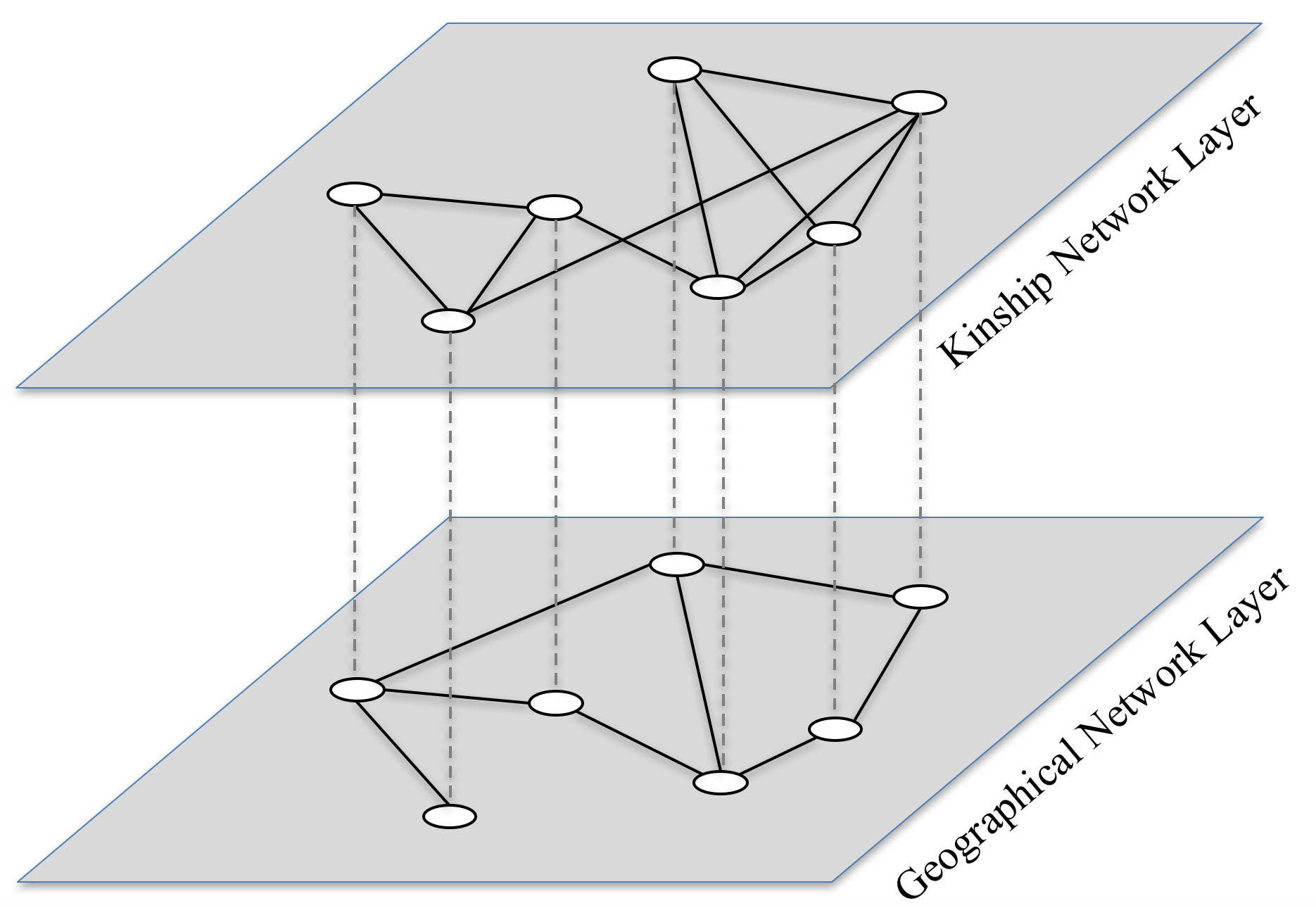
The agent-based model represents a village as a social network and the households in the village as nodes on the network. The social network consists of two layers. One is composed of kinship ties plus house neighbourhood ties or kinship ties - both cases are tested, and the other is composed of land plot neighbourhood ties. The two layers constitute a multiplex network, i.e., network with multiple relations among the same set of actors (see Figure 2). The diffusion takes place on the two layers simultaneously, and a household is considered as adopting once it has adopted on either layer.

We hypothesise that social learning takes place on the kinship (or kinship plus house neighbourhood) layer, whereas externalities on the land plot neighbourhood layer. They are represented by different approaches in the model. Two approaches are often utilised to model an agent's adoption decision. One is a probability based, wherein an agent's probability of taking an action changes as the proportion of his peers who have taken the action changes (e.g., Banerjee et al. 2013; Peres 2014). The other is a threshold based, wherein an agent takes an action as long as a certain threshold of the utility is reached (e.g., Granovetter 1978; Singh et al. 2013). In our case, a household's likelihood to adopt the new crop increased with the number of family members or house neighbours who had adopted. This decision-making process can be modelled following the probability-based approach. The probability for a household to adopt is thus proportional to the sum of the strengths of its kinship ties with those who have adopted. On the contrary, the externalities that adopting households' adoption behaviour imposed on non-adopters was mainly determined by the nature of the crop (such as its compatibility with the traditional crop). Such influence thus can be interpreted as a threshold that applies to all households, that is, a household will definitely adopt once the fraction of its plot neighbours that had adopted reaches a threshold. Therefore, externalities occurring on neighbourhood network is modelled using a threshold.

The agent-based model is a discrete-time model wherein each agent has one of two states at each time period, adopting or non-adopting. We treat the households who adopted in the first 2 years (2001 and 2002) as seed adopters. At the beginning of the simulation, seed adopters are in the adopting state. In each iterate period, the adopting agents remain in their state, whereas the non-adopting agents update their adoption states based on two rules corresponding to the mechanisms of social learning and externalities, respectively, as follows:

• (i) Social learning In each period, a non-adopter becomes adopting with a probability (elaborated below). The probability updates according to the proportion of his adopting peers on the kinship network in the last round.
• (ii) Externalities In each period, a non-adopter becomes adopting once the proportion of his adopting peers on the neighbourhood network reaches a threshold in the last period.

We now elaborate how the probability for a household to adopt is determined. Let \(p_{it}\) denote the probability that the household \(i\) adopts at time \(t\). It is a function of household's characteristics \(X_i\), time-varying factors \(Z_t\) and the effect of social learning \(F^{kin}_{it}\) (specifically, the proportion of the household \(i\)'s adopting peers over all peers on the kinship layer at the time \(t\)), given by

$$p_{i,t} = \Pr(\mbox{adoption}X_i, F^{kin}_{i,t}) = f(\alpha + X'_i \beta + Z'_t\gamma + \lambda F^{kin}_{i,t})$$

where \(f\) is assumed to be a logistical function that is widely used. It yields:

$$\log \left(\frac{p_{i,t}}{1-p_{i,t}} \right) = \alpha + X'_i \beta + Z'_t\gamma + \lambda F^{kin}_{i,t}$$

The threshold for externalities, \(h\), is a predefined ratio varying between 0 and 1. Households compare this ratio with the proportion of the household's adopting peers on the land layer \(F^{land}_{i,t}\). The household \(i\) adopts when \(F^{nei}_{it} > h\); otherwise, it remains unchanged.

The vector of household-level covariates, \(X_i\), consists of age of household head, number of farming workers and sum of path lengths to earliest adopters. Farming AS is a more labour intensive work than farming traditional crops, so a household's adoption behaviour was likely to be influenced by its abundance of labour. This is reflected by age of household head and number of farming workers. Considering the possible influence of earlies adopters, we include a covariate indicating household's social connection to the earliest adopters in its village. The time-varying covariate \(Z_t\) here only refers to last year's average price in the wholesale market.

In our case, households' adoption behaviour updated annually and the diffusion process lasted from 2003 to 2009. Accordingly, our model iterates on a yearly basis and the iteration proceeds for 7 years (the first 2 years are treated as the initial period in the model). The two effects occur simultaneously in reality, so we set the order to update them as random in the model. We repeat the simulation for 100 times and take the means of them for the output variables (e.g., adoption rate).

Model calibration

Calibration in this paper refers to setting values to parameters with real-world data. It is pertinent to the parameters that characterise households themselves and their behavioural environment. The three types of social networks, kinship network, house neighbourhood networks and land plot neighbourhood networks are calibrated with the actual networks in 2001 for each studied village. These networks are static during the diffusion process. The demographic characteristics for households are calibrated with the real data in 2001. They, except age (which grows each year), do not change over time. The distance to arterial road for each village is calibrated in the same manner. The price for each year is calibrated with the actual price in the corresponding year. The seed adopters in the model are aligned with those in 2002, the initial period of the simulation, for each village.

Model estimation

The task of estimation is to find the values for parameters so the output best fit data. There parameters, in our case, are those define households' behavioural process, i.e., the underlying mechanism of peer effects. Instead of simply finding the optimal value for each of the parameters, we obtain optimal values for each parameter by fitting the model to each of a large number of datasets (1000 in our case), which are generated by a statistical process (bootstrapping). With such a large number of optimal values, we can estimate the distribution of the optimal values and further determine whether the parameter matters in the behavioural process from a statistical perspective.

Specifically, the simulated adoption rate is compared to the observed adoption rate year by year (from 2003 to 2009) for each village. As there is no obvious way to determine the values of the parameters that would make the best fit, we conduct a grid search. Initially, we set a reasonably large space and search the space coarsely by large increments. We then narrow down the interval and search by smaller increments. We search over the entire discrete parameter space, denoted by \(\Theta\). For each grid point \(\theta \in \Theta\), we repeat the simulation 100 times, each time letting the diffusion run for 7 years (corresponding to the years from 2003 to 2009). The adoption rate at each year is collected in the simulations. We calculate the average adoption rate at each year over the 100 simulations subsequently. In a mathematical expression, \(\overline{Y}_{t,r}^{sim}(\theta) = \frac{\sum_{s=1}^S {Y_{t,r}^{sim}(s,\theta)}}{S}\), where \(Y_{t,r}^{sim}\) denotes the simulated adoption rate for the village \(r\) in the year \(t\), \(s \in [1, S]\) denote the index of simulation repetitions and \(S = 100\) in the present case. Next, we calculate the mean absolute errors (MAE) and choose the set of parameters that minimise the metric, given by

$$MAE(\theta) = \frac{1}{r} \sum_{r=1}^R {\sum_{t=1}^T {\vert \overline{Y}_{t,r}^{sim}(\theta) - Y_{t,r}^{emp} \vert}}$$

where \(Y_{t,r}^{emp}\) denotes the empirical adoption rate.

To estimate distributions of the optimal values of the interested parameters (i.e., the elements of \(\widehat{\theta}\)), we utilise a Bayesian bootstrap algorithm, which exploits the independence across villages. This method enable us to generate a large number (1000 in this case) of re-samples (i.e., bootstrap samples) out of the 10 village observations. Therefore, 1000 optimal values can be obtained for each parameter. The distribution of a parameter's optimal value can then be described.

Specifically, the model estimation is conducted in the following steps:

• (i) compute the deviation from simulated and empirical adoption rate, denoted by \(d\), for each of village \(r=1,\cdots, 10\), and at each parameter grid.

$$d(r,\theta) = \frac{1}{S} \sum_{s \in [S]}m_{sim,r}(s,\theta) - m_{emp,r}$$

• where \(m\) denotes the moment.
• (ii) bootstrap from the set of the 10 villages for 1000 times. All sample villages' deviations at each parameter grid are recorded.
• (iii) for each bootstrap sample \(b=1, \cdots, 1000\), calculate a weighted average of deviations, denoted by \(D\)

$$D(b) = \frac{1}{R} \omega_r^b\cdot d_r(\theta)$$

• where \(\omega_r^b = \frac{e_{br}}{\overline{e}_r}\), with \(e_{br}\) the i.i.d. exponential random variables and \(\overline{e}_r = \frac{1}{R}\sum e_{br}\).
• (iv) find the set of parameters that minimises MAE at each sample

$$\theta^* = \arg_{\theta \in \Theta} \min{MAE(\theta)}$$

We consequently obtain \(1000\) samples of optimal sets of the parameters, i.e., \(\{\theta^{*b}\}_{b \in [1,1000]}\). To conduct the statistical inference, we calculate the 95% confidence intervals of the interested parameters.

We first run the model with only the social learning mechanism, and then include the externalities mechanism. We refer to these models in terms of their parameters as follows:

• (i) Learning model: (\(p_{i,t}(\alpha, \beta, \gamma, \lambda)\))
• (ii) Learning-externalities model: (\(p_{i,t}(\alpha, \beta, \gamma, \lambda), h\))

In addition, the learning-externalities model is estimated by fitting the adoption rates of the first 4 years, the last 4 years and all 7 years, to understand the effects at the early, the late phase and the entire process.

Results

Fitness of models

Table 3 presents each village's mean of the absolute errors over all 7 simulation years for the optimal parameter combination that minimises the MAE defined above. It contains the values for all the 5 models that will be estimated in this study. The results show that all the values are smaller than 0.10, most are smaller than 0.05 and the average of the values is 0.03. This means, on average, the difference between simulation and real adoption rates is about 3%. Our models, therefore, provide very good fits to the observed data.

Table 3: MAE for the estimated models

	Learning Model		Learning-Externalities Model
	(Kinship)	(Kinship+House Neib.)	(All Years)	(First 4 Years)	(Last 4 Years)
Village 1	0.045	0.032	0.018	0.020	0.007
Village 2	0.007	0.007	0.056	0.067	0.063
Village 3	0.046	0.018	0.035	0.041	0.005
Village 4	0.055	0.056	0.022	0.024	0.002
Village 5	0.017	0.017	0.008	0.007	0.004
Village 6	0.020	0.020	0.031	0.021	0.011
Village 7	0.028	0.027	0.063	0.055	0.000
Village 8	0.071	0.060	0.088	0.105	0.023
Village 9	0.038	0.038	0.046	0.041	0.001
Village 10	0.009	0.010	0.008	0.006	0.001

Estimation results

Estimation results are presented in Table 4. Remember that parameter \(\lambda\) (in the logistical function) indicates the effect of social learning and parameter \(h\) reflects the effects of externalities. Panel A presents the results of estimating the learning model with adoption rates of all 7 years. The estimation is conducted first in the scenario that social learning solely occurs through kinship ties and then in the scenario that it occurs through kinship ties plus house neighbourhood ties. The parameter \(\lambda\) is significantly different from 0 in both scenarios, meaning that social learning imposes a significant impact on the adoption rates over the years. It takes place through both kinship ties solely, and kinship ties and house neighbourhood ties together (kinship and house neighbourhood are highly correlated in these villages according to Xiong & Payne (2017)). For the sake of comprehensiveness, subsequent estimations are based on kinship ties plus house neighbourhood ties.

Table 4: Estimation results

	\(\lambda\)	\(h\)
Panel A: Learning Model
Kinship	6.10
Standard Error	[0.56]
95% CI of Bootstrap Distribution	[3.84; 7.16]
Kinship + House Neib.	6.27	DEL
Standard Error	[0.57]
95% CI of Bootstrap Distribution	[2.97; 7.21]
Panel B: Learning-Externalities Model
All Years	5.60	0.32
Standard Error	[0.54]	[0.21]
95% CI of Bootstrap Distribution	[2.83; 6.34]	[-0.22; 0.91]
First 4 Years	6.80	0.24
Standard Error	[0.42]	[0.25]
95% CI of Bootstrap Distribution	[4.76; 7.30]	[-0.16; 1.13]
Last 4 years	4.10	0.48
Standard Error	[0.30]	[0.08]
95% CI of Bootstrap Distribution	[2.89; 4.98]	[0.14; 0.61]

Panel B presents the estimation results of the learning-externalities model that includes both effects of social learning and externalities. When the model is fitted to the adoption rates in the entire diffusion process (i.e., 7 years), the parameter \(\lambda\) is still significant, whereas the parameter \(h\) is not. This result holds when the estimation is conducted using the data of the first 4 years, and the influence of social learning is more prominent. However, externalities become significant when fitting the model to the data of the last 4 years, whereas the influence of the social learning, although still significant, substantially diminishes. Overall, the results suggest that social learning has significant impact on the entire diffusion process and mainly in the early phase, whereas externalities only significantly influences the diffusion in the late phase.

Robustness checks

Alternative fittings

One potential concern with these results is that the estimation approach inherits the correlated effects and endogeneity problems that plague any effort to estimate peer effects from observation data. To address this, we perform robustness checks by fitting the model to the adoption rates in different subgroups of households. The subgroups are determined according to whether a household belongs to the largest lineage in its village and the household head's age. They are as follows:

• Lineage Groups
  • (i) the percentage of households that adopt in the largest lineage
  • (ii) the percentage of households that adopt in the other lineages

• Age Groups
  • (i) the percentage of households whose heads are older than 40 years of age in 2000
  • (ii) the percentage of households whose heads are no older than 40 years of age in 2000

For each grouping method, we compare the simulated adoption rates for each subgroup in the year of 2003, 2005 and 2007 (thus there are \(2 \times 3\) 'moments' to fit) with the empirical data. The estimation results are displayed in Table 4. For both the lineage groups and age groups, the results that whether the estimated values of the two interested parameters, \(\lambda\) and \(h\), cross zero in the 95% confidence intervals are the same as in the original fitting. The significances of the parameters are consistent with those for the original fitting in both the learning model and the learning-externalities model. Therefore, the results we obtain in the original estimation are robust to these alternative fittings.

Table 5: Estimation of alternative fittings

	\(\lambda\)	\(h\)
Panel A: Lineage Groups	DEL
Learning Model	3.25
Standard Error	[0.32]
95% CI of Bootstrap Distribution	[2.54, 4.05]
Learning-Externalities Model
All Years	2.89	0.58
Standard Error	[0.40]	[0.26]
95% CI of Bootstrap Distribution	[1.82, 3.33]	[-0.32, 1.01]
First 4 Years	3.25	0.44
Standard Error	[0.30]	[0.36]
95% CI of Bootstrap Distribution	[2.82, 3.83]	[-0.14, 0.072]
Last 4 Years	2.75	0.62
Standard Error	[0.30]	[0.013]
95% CI of Bootstrap Distribution	[0.82, 2.33]	[0.46, 0.92]
Panel B: Age Groups
Learning Model	7.27
Standard Error	[0.62]
95% CI of Bootstrap Distribution	[5.50, 8.49]
Learning-Externalities Model
All Years	6.35	0.46
Standard Error	[0.52]	[0.34]
95% CI of Bootstrap Distribution	[5.82, 7.33]	[-0.12, 0.81]
First 4 Years	6.96	0.36
Standard Error	[0.65]	[0.38]
95% CI of Bootstrap Distribution	[0.82, 2.33]	[-0.32, 1.01]
Last 4 Years	5.37	0.58
Standard Error	[0.76]	[0.016]
95% CI of Bootstrap Distribution	[3.42, 6.33]	[0.36, 0.78]

Inter-village effect

Due to the geographic proximities, it is possible that the adoption behaviours of the households in one village is influenced by the households in another village. The most likely channel for the inter-village influence is the kinship ties between households in different villages. To estimate this influence, we implement another estimation with the inter-village ties included in the kinship networks. The results are presented in Table 6. In both models, \(\lambda\) remains significant and the externality effect remains not significant, which are exactly the same as in the original estimate. Meanwhile, the values of the parameters do not alter from the original estimation essentially. Therefore, we do not find evidence that the inter-village effect substantially changes the results obtained in the previous section.

Table 6: Estimation of inter-village effect

	\(\lambda\)	\(h\)
Learning Model	5.28
Standard Error	[0.52]
95% CI of Bootstrap Distribution	[4.58, 7.04]
Learning-Externalities Model
All Years	4.75	0.38
Standard Error	[0.46]	[0.36]
95% CI of Bootstrap Distribution	[3.32, 5.33]	[-0.12, 0.71]
First 4 Years	4.95	0.28
Standard Error	[0.30]	[0.26]
95% CI of Bootstrap Distribution	[0.82, 2.33]	[-0.30, 1.01]
Last 4 Years	4.12	0.62
Standard Error	[0.30]	[0.06]
95% CI of Bootstrap Distribution	[2.82, 2.33]	[0.12, 0.91]

Discussion and Conclusions

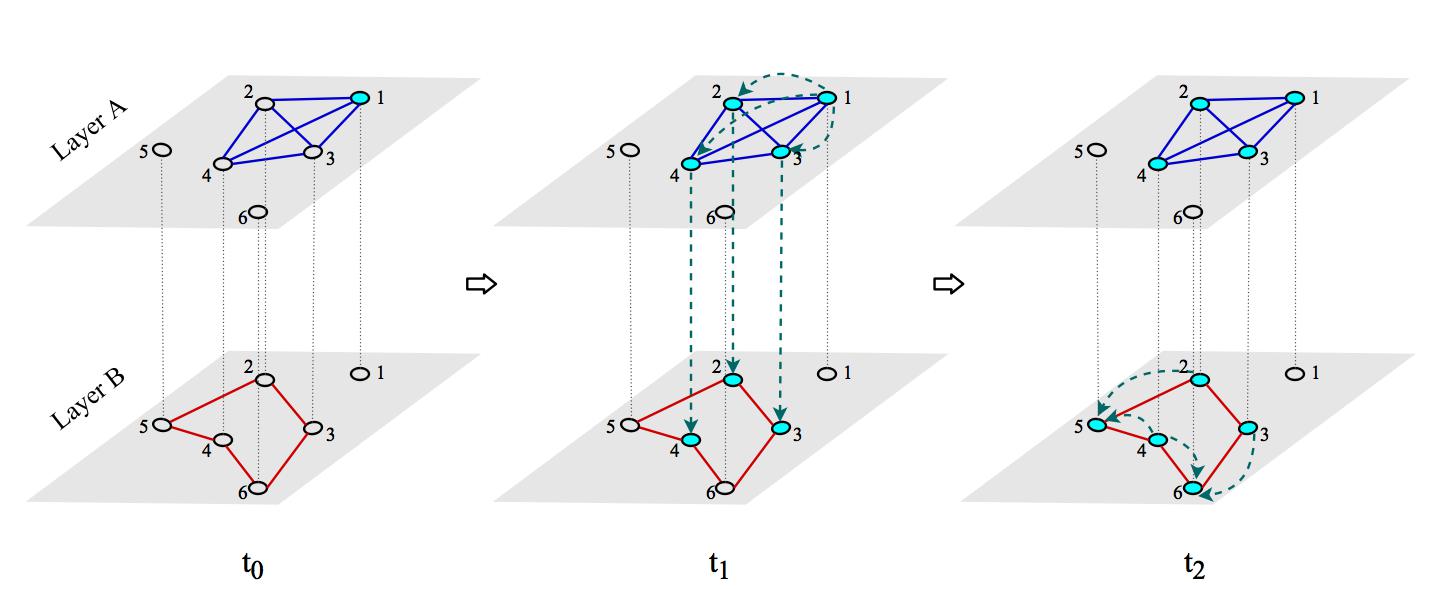
Our study identifies social learning and externalities in the diffusion of crops on rural networks. The two diffusion mechanisms take place through kinship ties plus house neighbourhood ties and land plot neighbourhood ties among the households, respectively. Social learning plays a significant role in the entire diffusion process and primarily in the early phase, whereas externalities only shape the late phase of the process. This shows that peer effects on a diffusion process can be caused by different types of interactions that take place through different social relationships at different stages of the diffusion process. In fact, the diffusion process is likely to be first triggered by the interaction on the social network of close relationships (e.g., kinship) and then further enhanced by the interaction on another social network. Such a process can be schematically illustrated by Figure 3. In this multiplex network, the diffusion starts on Layer A, where Note 1 motivates Note 2, 3 and 4 to adopt. Then the three new adopters motivate the remaining notes, 5 and 6 through interactions on Layer B.

The study has both methodological and policy implications. In the methodological aspect, it highlights the importance of understanding the interactive effects in social groups through the specific channels that facilitate the effects to occur. An effective approach is to distinguish the specific effects according to social relationships through which they transmit. A dynamic perspective is also needed as the roles that different channels play can vary as the diffusion proceeds. The diffusion achieved through one channel can trigger further diffusion through another channel. This study also demonstrates that agent-based simulation can be an effective approach to explore the underlying mechanisms of peer effects. It enables the explicit representation of multiple mechanisms on social networks. If the diffusion data from a number of samples are available, the significance of these mechanisms can be rigorously tested.

Our study also shows that successful diffusion can start at the dense social network that consists of the ties of a close relationship (e.g., kinship) and then reach the individuals the dense network does not cover through a different relationship. Therefore, giving priority to the promotion of the diffusion on dense and strong relationships can facilitate the diffusion in the entire social group efficiently. Specifically, in the case of Chinese rural communities, supporting the innovators in large lineages can be especially helpful for accelerating the spread of a new farming practice. Through the kinship ties, households can obtain information and resources that help them attenuate risks and reduce the initial cost. Once households adopting the new practice becomes the majority, the "laggards" are likely to be coerced to follow suit due to externalities imposed by the adopters.

In this work we move beyond the existing literature in several ways. First, in our model, the likelihood that an individual adopts the innovation depends on how likely he can obtain resources from earlier adopters and how much pressure it receives in coordinating behaviour with adopters. Existing studies generally either focus solely one diffusion mechanism or measure the overall peer effects by ignoring the nuance between different mechanisms in empirical analyses (save for Banerjee et al. 2013, which separates out the spreading of initial in-formation, but still leaves other mechanisms undivided). Such conflation can considerably bias the estimation, especially when the different mechanisms can o set each other (refer to Xiong et al. 2016a, for a simulation demonstration of such situation). Without explicitly modelling individuals' behavioural mechanisms, these effects are difficult to distinguish since they lead to similar results from a statistical point of view. In both cases, one with more peers who have adopted is likely to adopt himself. By simulating the interaction and decision-making at the individual level, we are able to separately estimate different underlying mechanisms of peer effects. Second, we identify the social relationships through which different effects take place. This is largely based on our in-depth observations in the study sites and good knowledge of the social fabric in these villages. We are able to empirically make the identification because we have access to the data of various social relationships in these villages, whereas data in such detail is rarely available for researchers, and thus we find no previous studies that empirically distinguish peer effects through different relationships. Third, we examine peer effects at different phases of the diffusion process. We divided the entire diffusion process into early and late phases, and check how each effect varies over the phases. Existing studies generally do not test such dynamics, assuming the underlying mechanism of peer effects is constant during the examined period. This is partially due to the difficulty of observing the entire diffusion process or a sufficiently long period of the process.

References

ABDULAI, A. & Huffman, W. E. (2005). The diffusion of new agricultural technologies: The case of crossbred-cow technology in Tanzania. American Journal of Agricultural Economics, 87(3), 645–659. [doi:10.1111/j.1467-8276.2005.00753.x]

BANDIERA, O. & Rasul, I. (2006). Social networks and technology adoption in Northern Mozambique. The Economic Journal, 116(514), 869–902.

BANERJEE, A., Chandrasekhar, A. G., Duflo, E. & Jackson, M. O. (2013). The Diffusion of microfinance. Science, 341(6144). [doi:10.1126/science.1236498]

BRAMOULLE, Y., Djebbari, H. & Fortin, B. (2009). Identification of peer effects through social networks. Journal of Econometrics, 150(1), 41–55.

BURSZTYN, L., Ederer, F., Ferman, B. & Yuchtman, N. (2014). Understanding mechanisms underlying peer effects: Evidence from a field experiment on financial decisions. Econometrica, 82(4), 1273–1301. [doi:10.3982/ECTA11991]

CENTOLA, D. & Macy, M. (2007). Complex contagions and the weakness of long ties. American Journal of Sociology, 113(3), 702–734.

CHRISTAKIS, N. A. & Fowler, J. H. (2007). The spread of obesity in a large social network over 32 years. New England Journal of Medicine, 357(4), 370–379. [doi:10.1056/NEJMsa066082]

COLEMAN, J. S., Katz, E. & Menzel, H. (1966). Medical Innovation: A Diffusion Study. Indianapolis: Bobbs-Merrill.

CONLEY, T. G. & Udry, C. R. (2010). Learning about a new technology: Pineapple in Ghana. American Economic Review, 100(1), 35-69. [doi:10.1257/aer.100.1.35]

DAHL, G. B., Løken, K. V. & Mogstad, M. (2014). Peer effects in program participation. American Economic Review, 104(7), 2049–74.

DEN BROECK, K. V. & Dercon, S. (2011). Information flows and social externalities in a Tanzanian banana growing village. The Journal of Development Studies, 47(2), 231–252. [doi:10.1080/00220381003599360]

FOSTER, A. D. & Rosenzweig, M. R. (2010). Microeconomics of technology adoption. Annual Review of Economics, 2, 395–424

GENIUS, M., Koundouri, P., Nauges, C. & Tzouvelekas, V. (2014). Information transmission in irrigation technology adoption and diffusion: Social learning, extension services, and spatial effects. American Journal of Agricultural Economics, 96(1), 328–344. [doi:10.1093/ajae/aat054]

GOETTE, L., Hu man, D. & Meier, S. (2012). The impact of social ties on group interactions: Evidence from minimal groups and randomly assigned real groups. American Economic Journal: Microeconomics, 4(1), 101–115.

GOLDSMITH-Pinkham, P. & Imbens, G. W. (2013). Social networks and the identification of peer effects. Journal of Business & Economic Statistics, 31(3), 253–264. [doi:10.1080/07350015.2013.801251]

GRANOVETTER, M. (1978). Threshold models of collective behavior. American Journal of Sociology, 83(6), 1420.

MANSKI, C. F. (1993). Identification of endogenous social effects: The reflection problem. Review of Economic Studies, 60(3), 531–542. [doi:10.2307/2298123]

MUNSHI, K. (2004). Social learning in a heterogeneous population: Technology diffusion in the Indian green revolution. Journal of Development Economics, 73(1), 185–213.

PERES, R. (2014). The impact of network characteristics on the diffusion of innovations. Physica A: Statistical Mechanics and its Applications, 402(0), 330-343. [doi:10.1016/j.physa.2014.02.003]

ROGERS, E. M. (1970). Diffusion of innovations in Brazil, Nigeria and India (No. 630.717 R6), Department of Communication, Michigan State University.

ROGERS, E. M. (2003). Diffusion of Innovations. New York, NY: Free Press, 5th edition.

ROGERS, E. M. & Kincaid, D. L. (1981). Communication Networks: Toward A New Paradigm for Research. New York, NY: Free Press.

RYAN, B. & Gross, N. C. (1943). The Diffusion of hybrid seed corn in two Iowa communities. Rural Sociology, 8, 15–24.

SINGH, P., Sreenivasan, S., Szymanski, B. K. & Korniss, G. (2013). Threshold-limited spreading in social networks with multiple initiators. Scientific Reports, 3, 2330.

VALENTE, T. W. & Saba, W. P. (1998). Mass media and interpersonal influence in a reproductive health communication campaign in Bolivia. Communication Research, 25(1), 96–124. [doi:10.1177/009365098025001004]

XIONG, H. & Payne, D. (2017). Characteristics of Chinese rural network: Evidence from villages in Central China. Chinese Journal of Sociology, 3(1), 74–97.

XIONG, H., Payne, D. & Kinsella, S. (2016a). Peer effects in the diffusion of innovations: Theory and simulation. Journal of Behavioral and Experimental Economics, 63, 1–13. [doi:10.1016/j.socec.2016.04.017]

XIONG, H., Wang, P. & Bobashev, G. (2018). Multiple peer effects in the diffusion of innovations on social networks: A simulation study. Journal of Innovation and Entrepreneurship, 7(2).

XIONG, H., Wang, P. & Zhu, Y. (2016b). Diffusion on social networks: Survey data from rural villages in Central China. Data in Brief, 7, 546–550. [doi:10.1016/j.dib.2016.02.081]

XIONG, H., Xiong, P. & Xiong, H. (2016c). KAMG: A tool for converting blood ties and affinity ties into adjacency matrices. Journal of Open Research Software, 4(1).