
Introduction
The concept of migration as an inherently social process has become crucial to explaining migration. (Roberts & Morris 2003; Arango 2004; Faist 1997; Massey & Espinosa 1997). Social network theory has been at the forefront of this change in perspective (Arango 2000, p. 291). Social network theory does not aim to explain how migration starts or why it might accumulate in one destination and not another. Rather, this theory concerns itself with the perpetuation of movement (Massey et al. 1998). Each additional migrant provides information and assistance to social ties who will, then, help their own contacts. In doing so, these ties help reduce the costs and risks of migration. Because network benefits are specific to the location where contacts reside, migration flows tend to be increasingly ‘siphoned off’ to already dominant destinations following the movement of others (Haug 2008; Hatton & Williamson 1998; Massey & Zenteno 1999; Epstein 2008, p. 5328). That is, “the deliberate or more ambiguous choices made by pioneer migrants... tend to have a great influence on the location choice of subsequent migrants, who tend to follow the ‘beaten track”’ (De Haas 2010, p. 1589).
Once a critical number of migrants have settled in a destination, migration adopts a self-perpetuating character whereby migration will continue independently of the conditions that led to its initiation, a process known as cumulative causation (MacDonald & MacDonald 1964; Lee 1966; Massey & Zenteno 1999; Light et al. 1993; Arango 2000; Castles et al. 2003). When cumulative causation has taken hold, the migratory flow between two countries will no longer be strongly correlated to macro-level variables such as wage differentials, employment rates or even government policy (Carrington et al. 1996; Faist 1997; Massey et al. 1993; Haug 2008; Arango 2000; Garip & Asad 2016). The effects of these macro-level variables will be “progressively overshadowed” by the role of networks in reducing the costs and risks of migration (Massey et al. 1993, p. 450). This prediction has important implications on governments’ role in shaping the global distribution of migrant flows because it implies that existing corridors between an origin and a destination will be resilient to immigration policy restriction; and that willing migrant destinations will have difficulty attracting migration from a given origin once a corridor from this source country has established itself elsewhere (De Haas 2010; OECD 2017; Czaika & De Haas 2014).
The concentration of immigrants from one origin in host destinations predicted by SNT is a widely-documented empirical regularity. Between 1980 and 1990, Western European countries received immigrants from the same traditional origins: North Africans migrated to France, while Turkish and Eastern Europeans migrated to Germany, for example (Collyer 2005). In 1990, 90 percent of all Hispanics lived in just 10 U.S. states, with 54 percent of all Hispanics concentrated in California and Texas (U.S. Census Bureau 1993). However, we also see evidence of migrant flows reorienting away from locations where co-ethnics have historically settled. In the 1960s, restrictive immigration laws in the United Kingdom reoriented migration from Caribbean countries to the United States and Canada which, at that time, were introducing relatively more favorable skill and education based immigration policies (Glennie & Chappell 2010). Within the United States, the emergence of new Hispanic destinations has been widely documented (Lichter & Johnson 2009; Leach & Bean 2008; Lichter & Johnson 2006; Terrazas 2011), with reorientation sometimes being attributed to non federal immigration laws (e.g. Ellis et al. 2014; García et al. 2011; Bohn & Pugatch 2015). Collyer (2005) finds that policy restrictions in France diverted Algerian asylum-seekers with France-based family networks to the United Kingdom.
The emergence of new migrant destinations among migrants from old source countries presents a puzzle for network theory. While SNT predicts path dependence, we know that the reorientation of migrants to alternative destinations also takes place. This paper develops an abstract theory-driven agent-based computational model (ABM) to examine the conditions under which network-based migration could display spatial reorientation. Calibration is an important consideration in ABMs because results obtained may be due to the specific values at which parameters are set. To limit modeler discretion, I anchor theory-driven parameter values to data from the widely-used Mexican Migration Project, which depicts Mexico-US migration from 1990-2013. I exogenously vary the immigration policies of two destinations: one with a sizable diaspora (the traditional destination) and one without (an alternative destination). I show that migration corridors driven by endogenous network dynamics can shift geographically as a response to policy conditions when we consider return migration. Out- and return migration helps the system update itself by allowing networks, and the benefits they bring about, to vary across space. Migration flows can then adapt to exogenous changes in immigration policy conditions and follow the path of least resistance to a new destination, which may eventually become dominant.
This paper makes several theoretical and empirical contributions. First, it contributes to furthering our understanding of the role of return – an understudied aspect of migration (King 2012, p. 13) – on the perpetuation of movement. Return migration involves moving back to the origin country permanently, or temporarily, in the case of circular migration (Boyd 1989). As in out-migration, networks play an important role for SNT. Networks in the origin country tend to increase the likelihood of return, whereas networks in the host country tend to decrease the probability of return (Haug 2008; Massey et al. 1987). In this paper, I propose that return migration has an alternative function in network migration: it can help a corridor contract and new inter-country linkages to be forged. At the micro level, it can allow migrants to adapt to changes in immigration policy by moving to alternative destinations. This prediction complements SNT and proposes one mechanism by which this theory may reconcile the existence of both path dependence and spatial reorientation found in the real world.
Second, migration theories generally seek to explain migration without considering the legal and political constraints that shape it (Arango 2000; Zolberg 1989; Hollifield & Wong 2000). As Arango (2000) suggests, “clearly, politics and the state are usually missing in theories of migration, and urgently need to be brought back” (p. 293). By considering the effects of immigration policy on the geographical distribution of migrants, this paper is contributing to this important gap in the literature.
This paper also contributes to the nascent field of agent-based modelling of migration (Klabunde & Willekens 2016). Agent-based modelling is, perhaps, one of the most suitable methods for exploring migrant adaptation to policy constraints and spatial reorientation. In the real world, if migration corridors emerge, they do so over several years. Dearth of evidence is compounded by the uniqueness of each case. Each corridor is formed as a result of a chain of different historical events, limiting our ability to understand the conditions under which corridors form, break or bifurcate. Agent-based modelling allows us to develop expectations about the real world by simulating how the system might behave under different scenarios, taking into account the effects of random variation on path dependent migration outcomes.
Furthermore, agent-based modelling allows us to explicitly model the dynamics described in theory. In line with the voluminous evidence supporting social network theory, migration possesses the main characteristics of a complex system. It is driven by individuals who interact locally to exchange information and resources, and these individuals form self-organising network structures (Massey et al. 1998; Willekens 2011; OECD 2009; Massey & Zenteno 1999). However, network dynamics are notoriously difficult to observe and test in the real world (Massey et al. 1994b) and agent-based modelling is the only method that permits the explicit modelling of social interaction (Klabunde & Willekens 2016). As such, many agent-based models of migration employ networks for the transmission of information (e.g. Espindola et al. 2006; Kniveton et al. 2011, 2012; Smith 2014; Hassani-Mahmooei & Parris 2012; Suleimenova et al. 2017; Klabunde et al. 2017), social capital (e.g. Silveira et al. 2006; García-Díaz & Moreno-Monroy 2012; Biondo et al. 2013), or both (e.g. Barbosa Filho et al. 2011; Klabunde 2014).
Much agent-based modelling of migration makes use of ABMs’ ease in simulating future or hypothetical scenarios. This is particularly true of recent studies on forced migration due to conflict and climate change (e.g. Suleimenova et al. 2017; Hattle et al. 2016; Hassani-Mahmooei & Parris 2012; Kniveton et al. 2011, 2012; Werth & Moss 2007; Entwisle et al. 2016; Smith 2014) but has also been applied to economic migration (Simon et al. 2018; Heiland 2003). Other studies make use of ABMs’ ability to explicitly model theoretical processes to test whether widely observed stylized facts can be replicated generatively. Some examples are Klabunde (2014), which develops an empirically calibrated ABM formalizing network theoretical predictions and is able to produce stylized patterns of geographical distribution and frequency of migration trips. Rehm (2012) uses agent-based modelling to investigate the relative influence of various economic and network variables in producing a wide range of migration signatures. Espindola et al. (2006) formalize the seminal Harris-Todaro economic model of migration (Harris & Todaro 1970) and find that adaptive, interacting agents can generate the key predictions of this theoretical model. Biondo et al. (2013) examines high-skilled migrants’ decision to return to the origin country, as a function of social capital and psychological variables. Klabunde et al. (2017) combines demographic transition rates and a psychological decision model to examine migration from Senegal to France.
This paper contributes to theoretical modelling of migration. First it expands the range of migratory behaviors and macro-level determinants that can be mimicked using ABM. I have identified only two models examining return migration, Klabunde (2014) and Biondo et al. (2013) and, to my knowledge, agent based models have not yet been used to explicitly examine the effects of immigration policy (with Suleimenova et al. (2017) and Simon et al. (2018) as notable exceptions). Second, agent-based models are an ideal platform for “complex thought experiments” (Cederman 1997). Existing theoretical ABMs of migration have used the method to explain the mechanisms by which predicted patterns are generated (e.g. Klabunde 2014; Rehm 2012), or to delve further into aspects of migrant decision-making which are poorly understood (e.g. Biondo et al. 2013). However, most agent-based models of migration have not, as of yet, attempted to subject migration theory to ‘stress tests’ as is done in other areas of study for example, war and conflict (Johnson et al. 2011) or microeconomics and trading (Epstein & Axtell 1996). Stress tests, which involve introducing or relaxing assumptions and testing the boundaries of theoretical expectations, is useful for theory refinement (Epstein 1999; Johnson & Groff 2014). This is particularly important for the theory at hand. Despite its prominence, “theorizing about migration networks has not gone beyond the stage of a conceptual framework” (Arango 2000, p. 292).
By formalizing SNT, this ABM aims to examine how network-driven migration can produce patterns that do not follow directly from basic theoretical premises. As such, it is designed to be an abstract depiction of a basic theoretical process that has been observed to operate in a range of migration systems such as European migration to the Americas in the 19th Century (Moretti 1999), migration within Europe (Haug 2008), the movement of Algerians to France (Collyer 2005) and the movement of Mexicans to the US (Massey et al. 1994a). The model is purposefully simplistic, allowing us to more easily attribute results to the theory at hand and, therefore, form general hypotheses about migration systems where networks have been observed to play a major role. However, calibration was based on a single case: the Mexico-US corridor between 1990 and 2013. Therefore, the results obtained are limited to this case and time period. Future work should parametrize the model with alternative cases.
Social Network Theory: Out- and Return- Migration
Migrant networks are sets of interpersonal relationships between migrants, non-migrants and former migrants spanning origin and destination areas. According to social network theory, aspiring migrants can derive several benefits from connections to established immigrants. In this section, I outline the main premises of SNT as they regard out- and return migration. I also outline the assumptions that will guide the computational model described in the next section.
Social networks are cost-reducing. Ties abroad provide information and resources that mitigate the costs of the move. Upon arrival, newcomers can draw upon established migrants to provide them with access to lodging, food and employment. In the case of Mexico-U.S. migration, cross-border connections between origin and destination communities are often institutionalized, for instance, through daughter communities or sports clubs in the U.S. These arrangements promote the frequent sharing of news and information between migrants and non-migrants, and provide a solid base for migration assistance (Massey et al. 1987). Korinek et al. (2005) documents the importance of ethnic enclaves in helping rural migrants navigate the difficulties of urban life in Thailand.
Social networks are risk-reducing. By helping new migrants access employment abroad, networks make migration an attractive strategy to diversify household income. Using data from a 2003 survey, Adams et al. (2005) find that money transfers made by migrants working abroad accounted for 15 percent of per capita household income in rural Mexico. According to Palloni et al. (2011), “[h]aving a tie to someone who has migrated yields social capital that people can draw upon to gain access to an important kind of financial capital, that is, high foreign wages, which offer the possibility of accumulating savings abroad and sending remittances home” (p. 1264). Having access to an alternative source of funds can provide the income security needed to stimulate labor activities that can be subject to adverse income shocks, such as agriculture. For instance, Wouterse & Taylor (2008) find that intercontinental migration of family members can increase livestock production among farmers in Burkina Faso.
Migration is self-perpetuating and overshadows macro-level conditions. When a critical threshold of migrants is reached, migration feeds future movement (De Haas 2010; Epstein 2008; Liang et al. 2008). As people migrate, they become a source for network benefits that future migrants can draw on. This induces further migration which, in turn, reduces costs for a further set of people, increasing their likelihood of migrating. Networks will have a larger effect on migration flows than wage differentials, employment rates or immigration policy. Migration can remain an attractive option despite negative employment or policy conditions due to the falling risks and costs of movement stemming from the growth of networks over time (Massey et al. 1993).
Social network theory does not make assumptions about whether individuals intend to migrate permanently or temporarily. It is a dynamic theory and holds that “acts of migration at one point in time systematically alter the context in which future migration decisions are made” (Massey et al. 1993, p.449). Individuals may set off with a particular migration goal in mind, but the location where their social networks are residing at a given point in time will play an important role in the decision to return or remain abroad. We can expect social networks to serve a similar facilitating function for return as they do for out- migration: reducing the costs of return and helping migrants secure employment or reintegrate in other ways (Haug 2008; Massey et al. 1987; Constant & Zimmermann 2012; Constant & Massey 2002; de Haas & Fokkema 2011; Klabunde 2014).
Networks in the origin country influence return flows. A 2015 Pew Research Center report indicated that six in ten Mexican return migrants considered reuniting with family at home to be the leading motivator for the decision to end their stay abroad (González-Barrera 2015). In a recent survey on Mexican return migration conducted in Jalisco, which has the highest return migrant population of the country, networks of family and friends are not only desired but relied upon for reintegration, given a lack of support services from government and other organizations (Mexicans and Americans Thinking Together 2013). In the case of Italian migrants in Germany, Haug (2008) finds that when migrants’ family ties return home, migrants themselves are more likely to return shortly after.
By the same token, networks in the host country will tend to decrease an individual’s probability of return (Massey & Espinosa 1997). Using a nationally representative longitudinal survey of German guest workers from major source countries, Constant & Massey (2002) finds that having a spouse or children in Germany strongly lowers the probability of returning, while having a spouse and children outside of Germany strongly increases it. Similarly, Haug’s (2008) single corridor study finds that the more social ties Italian immigrants accumulated in Germany, the less likely they were to return home. Massey & Espinosa (1997) ind that the migration of wives and children to the United States and the birth of children there was associated with a much lower probability of Mexicans returning to their home country.
Though SNT emphasizes networks’ role in facilitating return, it does not offer an explanation of return motivations. When (if at all) and why will a migrant wish to return to the origin country? Neo-classical Economic theory (NE) and the New Economics of Labor Migration (NELM) offer, perhaps, the clearest expectations on motivations for return. According to NE, individuals migrate to higher-wage locations in order to maximize expected net lifetime earnings (Sjaastad 1962). Return migration will happen only if expectations of employment and higher wages have not been met. According to the NELM, on the other hand, people migrate with the intention of returning. Migrants are conceptualized as “target savers,” a term which includes personal savings with the prospect of possible investment upon return, and remittances sent home (de Haas & Fokkema 2011, p. 759). Presumably, remittances will also be sent for savings and investment purposes if migrants are considering eventual return (Amuedo-Dorantes & Mazzolari 2010). Once migrants meet their ‘target savings’ they return home where, among other monetary and non-monetary advantages, they can enjoy the higher purchasing power of their foreign earnings (Constant & Massey 2002; Stark et al. 1997; Dustmann 2003). According to Boyd (1989), accumulating as much foreign currency as possible in a short period of time, with the aim of return, is a common migrant strategy. Individuals often migrate to save enough money to buy a home or invest in a small business in their home community (Massey et al. 1987). However, quantitative studies have found mixed support for NE and NELM and suggest return motivations are likely heterogeneous (Constant & Massey 2002; de Haas & Fokkema 2011).
This paper does not aim to test motivations for return migration. Instead, it aims to show the effects of return migration on geographical patterns by contrasting a model where migration is temporary to one where it is permanent. I implement NELM’s concept of ‘target savings’ to model return migration because NELM considers return to be intentional, while the neo-classical model explains return as the result of a miscalculation. That is, return migration under NE should only occur “if a migrant’s expectations for higher net earnings are not met – because of under- or unemployment, because wages are lower than expected, or because the psychic costs of moving are higher than anticipated (i.e., they find they unexpectedly miss their homeland, its culture, and its people)” (Constant & Massey 2002, p. 10). Secondly, the NELM framework can be considered complementary to social network theory (see, for example, Massey et al. 1993). Remittances – an essential risk-reducing mechanism within SNT – are an anomaly within NE, which expects that earnings are used to maximize migrant utility in the host country. Within the NELM framework, these private transfers play a key role (Constant & Massey 2002).
From these premises we can derive several assumptions to define agent rules:
- Agents will value destinations more highly if their networks have migrated there. Networks are key sources of information and benefits which reduce the costs and risks of migration to their area.
- Individuals migrate with the intention or goal of earning a foreign wage, saving, and sending remittances home.
- In an individual’s out-migration calculus, network benefits overshadow macro-level variables such as immigration policy and wage differentials.
- Agents’ return migration calculus will consider both ‘target savings’ and network benefits. Individuals tend to move to or remain in the location where they can draw on the benefits of network membership.
Even though immigration policy is not assumed to play a direct role in an agent’s calculus, it does affect decisions by limiting migrant inflow and, by extension, network benefits (assumption c). To show this, I simulate and vary a very simple immigration policy barrier, which I explain in more detail in the following section. Appendix A includes alternative models where agents receive direct feedback and learn from the policy environment. These results show that incorporating direct policy feedback does not enhance spatial reorientation[1].
Model Description
Reorientation to alternative destinations is a form of adaptation to adverse policy conditions. However, a large diaspora in the traditional destination can function as a magnet that “channels later streams of immigrants to the same location” (Massey 1999, p. 306). In this paper, I develop a conceptually simple ABM to demonstrate that migrant adaptation to policy change in network-driven migration can take place when we consider the effect of return migration on future flows.
The model is implemented in Netlogo – a state of the art multi-agent programmable modeling environment (Wilensky 1999). Geographic entities are abstract and the network structure stylized, while agent characteristics are empirically guided (Gilbert 2008). I opted for this strategy in order to anchor parameters to realistic values while maintaining a simple, theory-driven, architecture. I initialize 272 agents, with no two agents occupying a single cell (or grid square) at any given time. This number of agents was chosen to strike a balance between runtime, sample size and the exploration of a large parameter space. Equations operating at the macro-level are normalized by number of agents. Further details about how the number of agents was derived and additional tests using a larger number of agents can be found in Appendix B. I find that sample size does not significantly affect results.
When possible, agent variables are set by randomly drawing values from a distribution with empirical central tendency and dispersion parameters, as well as a shape similar to that shown in data. Input parameters are set using the Mexican Migration Project (MMP) dataset (mmp.opr.princeton.edu) and alternative sources. The MMP survey combines techniques from ethnographic and survey methodology, which obtain a wealth of valuable migration-related information. Communities are surveyed only once and are selected based on diversity in terms of size, ethnic composition and economic development, but not levels of out-migration (Massey & Zenteno 1999). Approximately 200 households are surveyed for the MMP in December-January each year.
The span of data used as inputs to this model is restricted to U.S. entries in 1989 – after the implementation of the sweeping Immigration Reform and Control Act (IRCA) – and before 2013. The Immigration Reform and Control Act, which was passed in 1986, reduced U.S. entries and exits by Mexican migrants and was powerful enough to herald a “new era of Mexican migration” (Durand et al. 1999). As such, I consider 1990, the year after IRCA implementation was finalized, to be a natural starting point for empirical calibration.
The network structure of Mexican communities is unknown. Therefore, I initiate the model using a stylistic small world network topology (Watts & Strogatz 1998) following simulation models of migration (e.g. Klabunde 2011; Fagiolo & Mastrorillo 2013). Small-world networks display high clustering like regular networks but also have small path lengths like random networks (Watts & Strogatz 1998). Since Watts & Strogatz’s seminal paper, studies have found that numerous real world networks exhibit small world properties (Telesford et al. 2011). Appendix C shows results using two alternative network structures: a random network (Erdős 1959; Gilbert 1959) and a regular network. Although these networks are unlikely to be found in real life (Barabási et al. 2016), this comparison allows us to explore the influence of stylized network properties on results. I find that connectivity is key. At first, only few individuals will migrate to the alternative location. For spatial reorientation to take place these migrants must be able to communicate efficiently with agents in the origin country. Network structures with low connectivity will inhibit such communication.
The small world network is specified following Wilensky’s (2005) implementation of this network in an agent-based model, which is based, in turn, upon Watts & Strogatz (1998)[2]. Once the network is formed, agents move to their starting cell, ready for the simulation to begin. Throughout a simulation run, the spatial position of agents changes with migration and return. However, the network arrangement remains constant for simplicity.
Social network theory considers both strong and weak ties to be important (Gurak & Caces 1992). Granovetter 1973) argues that close contacts in a social network are likely to have very similar information, and individuals are more likely to obtain new information through a more distant, weaker, connection. However, empirical literature on social networks in migration tends to emphasize strong family ties over weaker ones (King 2012; Collyer 2005; Angelucci et al. 2009). This is because strong ties are able to provide “thick information and active assistance” (Garip & Asad 2016, p. 1171). In this paper, I consider all ties to be strong. I set the median number of ties to 6. This number of ties was computed using the MMP dataset by summing respondents’ household members to their blood-related family members currently in Mexico – specifically uncles, cousins and nephews – and taking the median. I only have access to data on family members in Mexico who have been to the US before, likely limiting the size of the network. In Appendix D, I provide alternative results varying the number of ties from 4 – the median size of a Mexican household – to 10 the median size of an extended network using all network variables available in the MMP dataset. I find a small tendency for the likelihood of spatial reorientation to be reduced as the number of ties increases in number. In Appendix E, I conduct alternative tests where I differentiate between strong and weak ties. In these tests, I consider weak ties to be additional ties that are less likely to provide information and assistance than strong ties. In this simplistic conceptualization, I find that the inclusion of weak network ties does not enhance spatial reorientation.
Following Rossi (1955), migration decisions are taken within a simulated year. This means that, if an agent has decided to migrate to a destination \({k}\) and is successful, it must wait until the next year to decide whether to return home. By the same token, if the agent was not successful, it must wait until the next year to make another migration decision. There are several life-cycle events that may affect the timing of migration decisions: marriage, leaving one’s parental home, starting higher education, beginning a first job or having a child (Mulder & Wagner 1993; Mulder 1993; Kulu & Milewski 2007). Although a consideration of demographic transitions is important to the study of migration, these do not play a significant role in literature on social network theory and, as such, are not considered here. Doing so could overburden the model and make it difficult to obtain clear results when attempting to understand the theory in question (Bruch & Atwell 2013, p. 8).
The model abstracts the migration decision to be a function of only two variables: network benefits and expected wage (assumptions a - c in Section 2.10). Agents originate from a single location and can migrate to one of two destinations. If they are abroad, they may return to their home. The utility for return is a function of target savings and network benefits (assumption d).
Though conceptually simple, Figure 1 shows the model’s extensive macro, meso and micro level interdependencies and feedback. In this figure, agent calculations are distinguished by white boxes, macro-level or global processes are in blue, and meso-level feedback (information transmitted through networks), by gray shading. Let us look at out-migration decisions first (starting from “Networks” box). After setting current location and wage variables at the start of the simulation, individuals residing abroad relay information on these variables to network ties at home. This feedback will form the basis of these ties’ destination utility calculations (which, as mentioned, is a function of network benefits – or the presence of network members in a given location – and expected wage). Migrants also send remittances, which may help their home ties counter the costs of out-migration. An agent residing at home may decide not to migrate. If they do decide to migrate to a destination \({k}\), the potential migrant is subject to the financial costs of migration as well as the probability of being granted a visa.
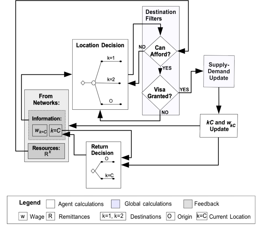
Two macro-level variables have direct or indirect effects on individuals’ ability to migrate at this stage: Immigration policy and average wage. Governments grant visas to some potential migrants and not others (in this simple model, all agents are equally likely to obtain a visa given a probability or quota). From the perspective of the non-migrant, the more restrictive the policy, the smaller the network living abroad is likely to be. At an aggregate level, restrictive immigration policies limit the stock of migrants in \(k\) – or the supply of labor – which, in turn, affects the average wage in this destination[3] (see “Supply-Demand Update” box). A change in the average wage has a number of implications at the agent level. It, primarily, affects the actual wage obtained by individual migrants. However, because migrants send information and monetary resources to their ties at home, it also influences non-migrants’ earnings expectations for the destination where their ties are located (and, therefore, their utility for migrating there), as well as the resources they have available to off set the costs of migration.
The decision to return will depend on the interplay of two factors: attaining a ‘savings target’ and the current location of network ties, following assumption d. As such, return decisions will be informed by network feedback on current location (see “From Networks” and “Return Decision” boxes). Finally, when return migrants update their location status, they will affect the out-migration utilities of their home-based ties. Specifically, migrants returning from destination \({k}\) will reduce home-based ties’ expected network benefits for \(k\). In what follows, I provide further detail on model processes.
Emigration and destination choice
The emigration procedures in this model are drawn from Epstein (2008) and follow the theory described in Sections 2.1 to 2.11. According to Epstein, an individual’s utility function, \(U_k\), for migrating to a particular location \(k\) depends on two variables: wage (\({w_k}\)) and networks present at that location (\({N_k}\)). Utility increases with respect to wages and with respect to the immigrant stock (for the benefits that networks entail). This is defined by the following partial differential equations:
| $$\frac{\partial{U_k}(w_k,N_k)}{\partial{w_k}} > 0, \frac{\partial{U_k}(w_k,N_k)}{\partial{N_k}} > 0$$ | (1) |
For a given utility, the size of networks and wages are substitutable. In other words, if wages drop, the migrant can be compensated by an increase in network size (Epstein 2008, p. 570).
| $$\frac{dw_k}{dN_k} = - \frac{\frac{\partial{U_k}(w_k,N_k)}{\partial{N_k}}}{\frac{\partial{U_k}(w_k,N_k)}{\partial{w_k}}} < 0$$ | (2) |
The wage in equilibrium is a function of the stock of immigrants in the country: as the stock of immigrants increases, the equilibrium wage decreases (Epstein 2008, p. 571). This is because migrants are assumed to come from the same origin country and will compete with one another. The assumption that migration negatively affects the income of immigrants who arrived in earlier years is supported by extant evidence (OECD 2017, p. 220) [4]. The wages that satisfy the equilibrium constraint are denoted by \({w_f^*}\) . The full derivative summarizing the utility, as a function of the equilibrium wage and networks, with respect to networks is described as follows:
| $$\frac{dU_k(w_f^*, N_k)}{dN_k} = \frac{\partial{U_k(w_f^*, N_k)}}{\partial{N_k}} + \frac{\partial{U_k(w_f^*, N_k)}}{\partial{w_f^*}} \frac{dw_f^*}{dN_k}$$ | (3) |
An increase in the size of the network at the destination has two opposing effects: a positive one through the increase in network benefits and a negative one via the decrease in wages. The first component of the right hand side of the above equation is positive, while the second is negative, reflecting these opposing effects. When (3) equals 0, the additional network benefits from one extra migrant equals the decrease in benefits coming from wages. After this peak is reached, the utility for migrating as a function of networks at the destination begins to decrease: “the probability of an individual migrating to a certain country has an inverse U-shape relationship, with regard to the stock of immigrants already in the host country” [p. 573].
As, following Epstein (2008), wages are assumed to fall with an increase in migrant stock, I define the equilibrium wage for destination \({k}\) (\({W_k}\)) as the negative linear function
| $$W_k= - \beta d_k+b$$ | (4) |
The y-intercept \(b\) is set to the mean U.S. wage from the MMP sample, for years 1990 to 2013. As the stock of immigrants, \({N_k}\), increases relative to available jobs, \({G_k}\). This ratio is denoted as \({d_k}\), wages decrease. The number of available jobs is equal to the total number of grid squares in each destination \({k}\). When all available jobs have been occupied, \({W_k = 0}\).
When agents migrate to a destination, they are assigned an individual wage randomly drawn from an exponential distribution (\({w_i^k}\)) with the mean equal to \({W_k}\), to approximate the distribution of wages for individuals surveyed by the MMP. That is, individuals are earning, on average, the equilibrium wage given the size of the immigrant labor supply. As the stock of immigrants increases, the equilibrium wage decreases and, thus, migration continues to be beneficial for the host country.
Agents at the origin can only obtain information about host country conditions from the migrants they are connected to through network ties. Let \({x_{ij}=1}\) if a tie exists between decision-maker \({i}\) and agent \({j}\), and \({x_{ij}=0}\) otherwise. We then define \({X_i=\{j\in I | x_{ij}=1\}}\), which is the set of all connections between decision-maker \({i}\) and persons \({j}\) from all agents \({I}\), and \({X_i^k=\{j\in I_k | x_{ij}=1\}}\), which is a subset of \({X_i}\) including only agents who are in location \({k}\). Agents at home construct their expected wage value \({E(w_i^k)}\) as the average wage of network contacts living in destination \({k}\).
| $$E(w^k_i) = \frac{\sum\limits_{j \in X^k_i} w^k_j}{|X^k_i|}$$ | (5) |
Network benefits form the second component of the emigration utility function. Newcomers can derive benefits from migrants they are connected to through social ties and will therefore be drawn to the location where these migrants reside. By the same token, an individual will have greater home bias when a smaller proportion of his or her network has migrated, consistent with assumptions a and d (Section 2.10 above). As such, I define the network term \({N^k_i}\) as the proportion of total network contacts living in destination \({k}\) as:
| $$N^k_i = \frac{|X^k_i|}{|X_i|}$$ | (6) |
Having defined its two components, I describe the final emigration utility function, \({U^k_i}\), following Epstein (2008).[5]
| $$U^k_i = cE(w^k_i) \cdot \log(aN^k_i + 1)$$ | (7) |
| $$U^h_i = 1-\Bigg(\frac{\sum\limits^K_{k=1} U^k_i}{K}\Bigg)$$ | (8) |
In conclusion, the decision to migrate consists of three steps. First, the agent will choose to reside in the location with the highest utility, including home. If there is no single winner, agents will select a location by randomly choosing across the highest valued options. Second, having chosen their destination, agents at the origin will migrate if their accumulated wealth in the current year, \({\Lambda_{i,t}}\), is larger than or equal to the cost of migration \({\zeta_m}\). I explain how \({\Lambda_{i,t}}\) is constructed in the following paragraphs. The costs of migration include one month of destination country income forgone while transitioning into the new labor market, as well as transportation and visa costs. Third, agents will encounter a 'policy filter', whereby they will migrate subject to a probability of attaining a visa. Financial cost is an important consideration when migrating. However, I keep costs fixed across destinations to observe the unique effects of varying policy restriction.
Once abroad, all agents in destination \({k}\) spend their yearly (\({t}\)) wages, \({w^k_{i,t}}\), on food and lodging (consumption), \({C_{i,t}^k}\). They may also send remittances \({R_{i,t}^k}\). Remittances are private transfers between migrants and non-migrants (World Bank 2018). Theoretically, remittances may be sent from migrants to individuals in the origin country or vice-versa. I only consider transfers from migrants to residents. Agents identify one home country recipient at random, upon migrating, and maintain this recipient throughout the simulation run.
The proportion of a migrant agent's wages dedicated to consumption and remittances is equal to the median proportion of yearly destination country wages consumed and remitted, respectively, by MMP respondents across all relevant years. Yearly wages not spent on consumption and remittances (on average a little more than half the agent's yearly wage) is saved.
Savings at the destination, \({s^k_{i,t}}\), is given by:
| $$s_{i,t}^k = s_{i,t-1}^k + w^k_{i,t} - (C_{i,t}^k + R_{i,t}^k)$$ | (9) |
Agents in the home country accumulate savings in a similar fashion. However, instead of sending remittances, they may receive remittances, \(R_{i,t}^h\), from a network tie. Savings at the origin country computed as:
| $$s_{i,t}^h = s_{i,t-1}^h + R_{i,t}^h + (w^h_{i,t} - C_{i,t}^h)$$ | (10) |
Data on Mexican consumption was not available. As such, I assume non-migrant agents consume \((C_{i,t}^h)\) the same proportion of their wages (\(w^h_{i,t}\)) as migrant agents. Individuals who have migrated before maintain the savings they accumulated abroad, \({s_{i,t}^k}\), and are able to use these savings in addition to any they accumulated at home to re-migrate. Total wealth, \({\Lambda_{i,t}}\), is given by adding \(s_{i,t}^k\) to \(s_{i,t}^h\).
| Variables | Values | Equations | ||
| Empirical Parameters | Savings & Wealth | \({s^k_{i} (w^k_{i},C^k_{i},R^k_{i})}\) | 9 | |
| (fixed) | \({s^h_{i}(w^h_{i}, C^h_{i},R^h_{i})}\) | 10 | ||
| \({\Lambda_{i}}(s^h_{i}, s^k_{i})\) | 9,10 | |||
| Wage variables | \({w_i^k: X \sim Exp(W_k),}\) | 4,5 | ||
| \({0 \leq W_k \leq \mu^k}\) | ||||
| \({\mu^k = 22,075}\) | ||||
| \({w^h_i: X \sim Exp(\mu^h)}\) | ||||
| \({\mu^h = 4,502}\) | ||||
| Consumption | \({C^d_i = 0.25 w^d_i}, d = k, h\) | 9,10 | ||
| Remittances | \({R^k_i = 0.19 w_i^k}\) | 9,10 | ||
| \({R^h_i = 0.19 w_j^k}\) | 9,10 | |||
| Avg. number of ties | \({\gamma = 6}\) | |||
| Endogenous Variables | Networks (proportion) | \({0 \leq N^d_i \leq 1}\), \(d = k, h\) | 6,11 | |
| Exogenous Variables | Probability of Forming Random Tie | \({\pi = 0.25}\) | ||
| Financial Costs of Migration | \({\zeta_m : X \sim Exp(\mu_{\zeta_m}),}\) \({\mu_{\zeta_m} = 2,197}\) | |||
| Costs of Return | \({\zeta_r: X \sim Exp(\mu_{\zeta_r}),}\) \({\mu_{\zeta_r} = 441}\) | |||
| Savings Target | \({\eta = 2,846}\) | 11 | ||
| Pr. Entry | \({0 \leq P(Success) \leq 1}\) | |||
| Pr. Return | \({0 \leq P(Return) \leq 1}\) | |||
| Notes: \({\zeta_m}\) include one month of destination income forgone while transitioning into the new labor market, transportation and visa costs from Klabunde (2011) and U.S. Department of State (2015), respectively. \({\zeta_r}\) include one month of home country income forgone while reintegrating into the home labor market and transportation costs. All other fixed parameters are from MMP. All monetary units are in United States Dollars set using the Consumer Price Index for 2012 as the base (U.S. Bureau of Labor Statistics 2012) except for time-invariant variables. | ||||
Return migration
I model return migration utility, \({U^r_i}\), as a function of (1) the benefit of an additional network tie residing in the home country and (2) the benefit of approaching savings target \({\eta}\) (assumption d). These are the first and second components, respectively, on the right hand side of Equation 11. As both components are necessary for return, utility is modeled multiplicatively:
| $$U^r_i = \frac{\log(aN^h_i + 1)}{\log(a + 1)} \Bigg(\frac{2}{1 + \exp(-bs^k_i)} - 1\Bigg)$$ | (11) |
\({N^h_i}\) is defined as the proportion of ties to individuals in migrants’ home location over their total number of connections. All else equal, the larger \({N_i^h}\), the larger the motivation to return. On the other hand, if the number of migrants at home is small, either a large portion of friends and relatives have joined the migrant or moved to other locations and cannot help the migrant to reintegrate. Alternatively, the migrant may have never had a large network at home.
The savings target agents strive towards, \({\eta}\), is obtained from aggregate MMP data. I construct \({\eta}\) by adding return savings and remittances for savings and investment purposes accumulated throughout the length of stay of returned survey respondents, and taking the median across the sample[6]. Agents may be satisfied with saving an amount of money that is ‘close enough’ to the savings target, while not fully reaching it. As such, the utility for approximating is modeled as a logistic function (scaled and shifted such that the inflection point is at the origin) to reflect the diminishing marginal utility of approaching a concrete savings target. Equally – and consistent with network benefits in the emigration utility equation – the added benefit each additional home-based social tie can bring the agent is also marginally decreasing.
To solve for constants \({a}\) and \({b}\), I hold the second utility component at the savings target, \({\eta}\), and find two reasonable values or ‘anchor points’ for the first utility component – network benefits – in terms of \({U^r_i}\). If the amount of savings accumulated equals \({\eta}\), we would expect the utility of returning home, \({U^r_i}\) to be highest when the proportion of network ties residing at the origin, \({N_i^h}\), is also highest. Hence, when \({N_i^h = 1}\), I set \({U^r_i}\) to \(0.9\). When \({N_i^h = 0.3}\), \({U^r_i = 0.6}\), slightly above the midpoint. This reflects that, even if target savings have been met, having few network members at home has a discouraging effect. The largest possible value of \(U^r_i\) is \(1\). I conduct sensitivity tests varying parameters \({N_i^h}\) and \({U^r_i}\) across all possible values to obtain alternative anchor points. These tests, shown in Appendix F, indicate that the value of these anchor points does affect the average time migrants spend abroad. However, it does not substantially affect agents’ tendency to reorient to alternative destinations.
If able to pay the costs of return, \({\zeta_r}\), individuals return subject to the outcome of a Bernoulli trial, \({P(Return) \sim B(1,U^r_i)}\). Upon returning, agents can emigrate again the following year. In this model, agents who have returned are no different from those migrating for the first time. This is a simplification: migration can help individuals accumulate social capital abroad and will likely increase their changes of re-migrating. In Appendix G, I examine a model where agents with more migration experience are more likely to re-migrate than those with less migration experience. These tests show that when a proportion of agents have a lower probability of re-migrating (that is, agents with less migratory experience), reorientation is slightly less likely. However, results are robust to this change in agent rules.
Results
Network theory predicts that, once a critical mass of migrants have established themselves in a destination, they help channel future flows to the same destination. At this point, migration corridors will be robust to changes in governments’ attempts to influence movement (De Haas 2010; Massey et al. 1993; Garip & Asad 2016). I have argued that policy can lead to the reorientation of flows in the presence of return migration. Return migration can aid the system’s adaptation, allowing corridors to more easily shift to the destination that offers the greatest possibility for successful entry.
To test this, I present a scenario where a migration corridor has been established between the origin and the traditional destination (\(k=1\)), while comparably fewer migrants have settled in the alternative destination (\(k=2\)). That is, destination 1 is dominant. Specifically, I place 30 percent of all agents in destination 1 at initialization, and only 4 percent in destination 2. Across simulation runs, I vary the probability of a migrant gaining entry to both destinations (\({Pr(Success) k=1}\) and \({Pr(Success) k=2}\)) from 0 to 1, at intervals of 0.02 – small enough to observe granularities or non-linear effects that may emerge.
At initialization, the traditional destination is, of course, dominant. However, if individuals begin to move to an alternative destination, their social ties, drawn by network benefits, may subsequently follow the same path. If more individuals migrate to the alternative destination than to the traditional one, a new dominant destination is established. The relative dominance of destination 2 compared to destination 1, \({S_t}\), is measured by subtracting the proportion of migrants in the traditional destination, \({N^1_t}\), to those in the alternative destination, \({N^2_t}\), at a given point in time \({t}\). It is defined as follows:
| $$S_t = \frac{N^2_t - N^1_t}{N^1_t + N^2_t}$$ | (12) |
Given the initialization settings described above, \({S_t}\) at the start of a simulation run will equal -0.76. The value of \({S_t}\) increases as migrants reorient to destination 2 and will be positive if destination 2 becomes dominant.
I begin by showing patterns at a single point in time – at the end of 24 years – and then examine inter-temporal variation. I run models 1000 times per unique destination policy combination and display the average across these runs. I start each simulation run with a specific immigration policy setting and maintain this policy constant throughout 24 simulated years, matching the span of the input data. All parameter values not discussed in this section are shown in Table 1.
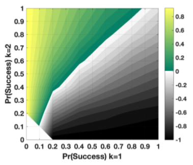
In the first set of results, I compare experiments where return migration is disabled and where it is enabled to show its unique effects on migrant reorientation. I examine migrant reorientation at the end of 24 years for different immigration policy settings. Figure 2a displays results where return migration is turned off and Figure 2b shows a model where return migration is enabled. For visual clarity, I use gray scale tones to depict values of \({S_{t=24}}\) that are below zero (that is, the proportion of migrants in the, traditional, destination 1, continues to be larger than in destination 2) and positive values of \({S_{t=24}}\) (destination 2 has become dominant) are shown in green hues. Within these two color ranges, lighter shading indicates higher values of \({S_{t=24}}\), or greater reorientation to destination 2.
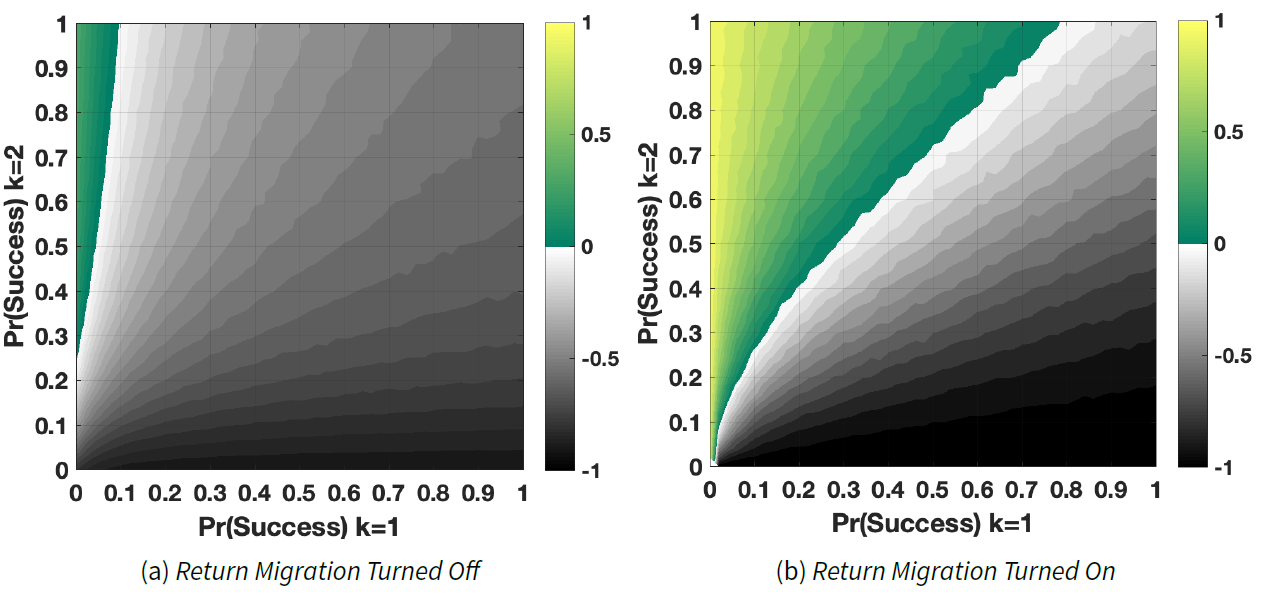
Figure 2a shows that, for the most part, individuals migrate to the traditional destination, regardless of the policy setting, when return migration is turned off. This is in accordance with the expectations of SNT. Destination 2 becomes dominant only when the traditional destination is extremely restrictive. Even when destination 1 closes its borders completely, the alternative destination must admit a minimum of 1 in 4 migrants to become the new dominant destination. Otherwise, migrants will persist in their attempts to follow their social ties to destination 1.
When policy in destination 1 is most restrictive and policy in destination 2 is most liberal, destination 2 accumulates 34 percent more migrants than destination 1 at the end of 24 simulated years. However, reorientation from the traditional to the alternative destination decreases sharply as destination 1 relaxes restrictions even slightly. When the probability of successful entry into destination 1 is relaxed from 0 to just 0.08, \({S_{t=24}}\) drops from 0.34 to 0. In other words, as soon as destination 1 accepts 8 percent of all migrants, destination 2 – despite accepting all migrants – loses its dominance.
Figure 2a shows that return migration has a significant effect on the reorientation of flows. A cursory look at the grid surface shows a substantial tendency for the alternative destination to replace the traditional one. The upper left triangular of the grid displays values of \({S_{t=24}}\) that are mostly larger than 0. Where the dominant destination is at its most restrictive and the alternative at its most liberal, destination 2 effectively replaces destination 1 as the sole migration corridor (\({S_{t=24} = 1}\)). It is only when the probability of entry into destination 1 is equal to or surpasses 78 percent that shifts in destination dominance cease to occur. Return migration allows the migrant stock in both destinations to vary in the presence of policy inequality. When the probability of being granted a visa to the traditional destination is low, migrant agents will return and stay home, reducing the number of migrants in destination 1. In this restrictive scenario, potential migrants in the origin are also unable to replace those returning home. With these two effects taking place, we might expect migration to cease completely. However, as the traditional corridor is contracting, changes are occurring at the micro and meso levels, which will increase the migrant population in destination 2. Return migration affects the locational composition of some agents’ networks and may tip these agents’ decisions in favor of the alternative destination. These individuals, in turn, may spur network migration towards the alternative destination. Through this process, the system can adapt and corridors can shift in response to hostile policy conditions.
However, destination 2 will not always be able to attract migration when the traditional destination restricts its borders. Figure 2b shows that the relationship between policy restrictiveness in the traditional destination and the value of \({Pr(Success) k=2}\) required to make the alternative destination dominant is non-linear. Counterintuitively, the alternative destination will have more difficulty becoming dominant when immigration policy in the traditional destination is extremely restrictive. This is because, as individuals’ networks are mainly based in the traditional destination, potential migrants will persist in their attempts to move to a destination they are unable to access. With no migration taking place, individuals are not able to reap the financial benefits of migration to re-migrate or help other aspiring migrants mitigate the costs of movement through remittances. However, if the traditional destination loosens its entry policy by a only small amount, becoming dominant becomes much easier for destination 2. When the probability of entry in destination 1 is just 2 percent, destination 2 must be willing to admit approximately 5 times more migrants to become dominant. By comparison, when \({Pr(Success) k=1}\) is 10 percent, destination 2 needs to admit 2.6 times more migrants than destination 1 to become dominant. When \({Pr(Success) k=1}\) is 20 percent, it needs to admit only double that of the traditional destination.
The average number of migratory trips an agent takes to destination 1 decreases proportionally to the probability of entry into this destination. In the simple case where destination 2 is completely closed off, agents in Figure 2b make an average of 5 migration trips in a 24-year period if they are able to enter the traditional destination when they please. As we restrict migrant entry to destination 1, however, agents are able to return home freely but not necessarily re-migrate. If half of all applicants are granted a visa, agents will make 3 migration trips to destination 1, on average. When 1 in 10 agents are accepted, agents will only make one migration trip, on average, throughout the 24-year period. In Figure 2b, agents’ length of stay averages between 1.15 and 1.35 years across all policy settings. These short trips should enhance the rate at which the system is able to adapt and corridors can shift. However, Appendix F shows that these results are robust to stays abroad of 2-5 years.
In real life, several factors may inhibit our observation of spatial reorientation. First, we may not be able to observe extreme differences in policy across major labor importing countries (Hollifield et al. 2014). As an illustration, let us consider the case where country 1 grants a visa to 8 percent of applicants (the probability of a Mexican applicant obtaining a U.S. green card in 2012 was 7 percent, according to MMP data). In order for country 2 to become dominant, it must grant a visa to 24 percent of applicants from this origin country in a given year – more than 3 times the percent admitted in country 1. In real life, this scenario may be unlikely. If destination 2 is desirable for migrants and has a similar demand for labor as destination 1, destination 2 may also impose restrictive policy measures.
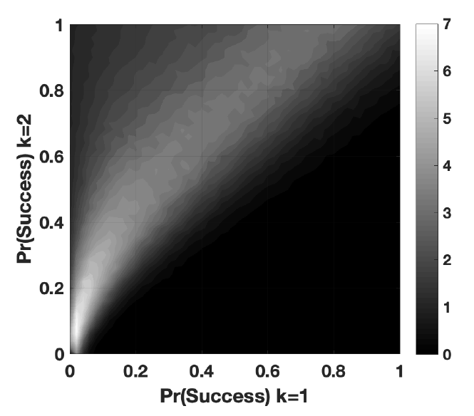
Second, if the dominance of one destination over another fluctuates over time, the policy impacts we observe will be dependent on the point in time at which we look. The following set of results examine fluctuations in destination dominance over time. Figure 3 displays the average number of times, within a 24-year run, where differences between the stock of migrants in destination 1 and destination 2 cross zero. Lighter hues signify a larger number of crossovers, or number of times dominance fluctuates from one location to the other. The average number of crossovers in the parameter space delimited by \({Pr(Success) k=1}\) \({< Pr(Success) k=2}\) – that is, where the alternative destination is more liberal – is 2.6. The highest activity is concentrated at low values of \({Pr(Success) k=1}\) and \({Pr(Success) k=2}\), where there may be up to 7 crossovers in 24 years. Overall, dominance shifts more frequently when entry policies in both destinations are similar. This is because migrant stock tends to become equal across destinations over time. This convergence, in turn, generates more indifferent potential migrants choosing destinations at random. In the area where \({Pr(Success) k=2}\) is decisively larger than \({Pr(Success) k=1}\), the number of crossovers decreases substantially. The remaining parameter space (the bottom-right triangular of the grid) is very stable (0.17 crossovers on average), indicating that agents are continually moving to destination 1, where a majority of migrants were placed at initialization. In addition to being affected by the policy setting, the number of fluctuations across the simulation is also affected by network size. In Appendix D, I show additional tests varying the average number of ties agents have. Larger networks result in agents’ destination utility being less sensitive to the movement of few individuals. Therefore, we see fewer corridor fluctuations. The maximum number of corridor fluctuations that can be observed across policy settings when \(\gamma= 10\) is 5.72.
Agents have networks with different locational compositions and are affected by random migration events which can generate distinct path dependent outcomes. As such, new corridors to destinations with lower immigration restrictions may not always establish themselves or may display a high degree of instability over time. Figure 4 displays a range of migration patterns that emerge over time when destination 1 admits 8 percent of migrants and destination 2 admits 80 percent. This setting was chosen because it generates a low average number of fluctuations in destination dominance (1.69, see Figure 3), making results easier to visualize.
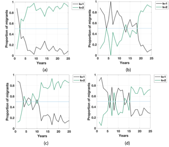
Figure 4a shows the case of a simple crossover taking place in the third year of the simulation. This is, by far, the most common fluctuation pattern for this policy combination. A visual inspection of a random sample of 50 runs (out of 1000) for this parameter combination shows that, in 74 percent of runs, once destination 2 becomes dominant, it stays dominant. In 76 percent of runs, all fluctuations take place by the fifth year. However, in a minority of cases, corridor fluctuations continue to occur well after year 5. Figure 4b shows a case where the proportion of migrants in both locations is equal at year 4 but destination 2 does not become dominant. Instead we see some instability occurring as late as year 13 before the alternative corridor finally establishes itself in year 17. Figure 4c shows a case where destination 2 becomes dominant in year 3, as in Figure 4a but then quickly loses its dominance the following year. After 5 shifts in rapid succession, the alternative corridor gains a stable dominance in year 10. Figure 4d displays a case where instability remains high across the simulation run.
Discussion
Network theory holds the risk and cost reducing effects of social ties make migration difficult for governments to control (Massey et al. 1993). This implies that once a migration corridor has been established, flows will not reorient to an alternative destination when immigration policy becomes restrictive (De Haas 2010). However, while the concentration of immigrants from one origin in host destinations is widely documented, studies have also shown that new migrant destinations can emerge in response to immigration policy (e.g. Collyer 2005; Bohn & Pugatch 2015). I develop a theory-driven agent-based computational framework upon which to examine the conditions under which network-driven labor migration could display spatial reorientation. In this model, agents are given the choice between the traditional destination – defined by a sizeable diaspora – and one with a very small number of settlers.
In line with social network theory, results show that migrant agents tend to cluster in the traditional destination even when policy conditions strongly favor movement to the alternative destination. However, when return migration is taken into account, migration flows are able to shift in response to policy conditions. In the presence of return migration, a liberal alternative destination can attract a higher number of migrants than a restrictive traditional destination. Results also show that the process of spatial reorientation can be highly unstable when both destinations have similar policies. Because the proportion of agents being admitted is similar across the two destinations, diaspora size is more likely to converge as agents return and re-migrate. This, in turn, generates similar migration utilities across destinations and, consequently, ambivalence in destination choice and instability at an aggregate level.
This paper contributes to literature seeking to understand the wide-ranging effects of immigration policy and does so from the perspective of network theory, which has, to date, provided one of the most recognized explanations for why migrants from a given origin form geographical clusters in host countries or regions (Epstein 2008). This ABM aims to extend the explanatory power of network theory by demonstrating a simple mechanism whereby migrant flows can reorient to the destination promising easier entry, as has been observed in empirical cases. In this model, return and re-migration shrinks the size of the traditional diaspora, allowing an alternative destination to compete. However, we could also see a geographic dispersal of an immigrant cluster driven by, for example, socio-economic mobility (De Haas 2010, p. 1611). In this situation, network benefits would no longer be spatially concentrated and, thus, neither would future migration. Alternatively, established immigrants may be prompted to change their behavior due to restrictive policy (e.g. Collyer 2005), dire economic conditions, or simply assimilation (e.g. Guarnizo et al. 2003, p. 1215), such that incoming migrants are unable to mobilize social capital. In this case, migration to the traditional destination would no longer occur regardless of the size of its diaspora. Further theoretical explorations of this kind would benefit from abstract thought experiments in agent-based modelling.
The simple model presented in this paper will also lay the foundation for future work exploring individuals’ complex interactions with immigration policy. Spatial reorientation is just one of a wide range of ‘substitution effects’ resulting from trade-offs in decision-making when faced with tough entry laws (De Haas 2011). One such effect is undocumented migration. Undocumented migration weakens the effects of visa restrictions and can, therefore, make spatial clustering more resilient to governments’ attempts to shape migration flows. Individuals might also extend the duration of their stay abroad in response to policy. Several studies have observed that individuals consider whether they will be able to re-enter the U.S. before they decide to return, resulting in prolonged or permanent migrations (e.g. Durand et al. 1999, Massey et al. 2016, De Haas 2011). By dampening return migration, this behavior could also limit the rate of spatial reorientation. Future extensions of this simulation model will seek to factor policy tightening into return intentions and allow for undocumented movement to take place. Future work will also expand the factors considered in migration decision-making beyond the simple utility calculation presented here. In reality, potential migrants consider a host of different factors that may or may not be a function of networks (Baláž et al. 2014).
There is a growing literature using agent-based models to examine policies in arenas such as economic policy (Brenner & Werker 2009), downtown revitalization (Ma et al. 2013), and immigration policy (Simon et al. 2018). Agent-based models are uniquely equipped to inform policy by allowing us to experiment with hypothetical scenarios in a virtual world, develop expectations on complex policy outcomes, and help us design smarter policies that limit their unintended effects (Gilbert et al. 2018; Simon 2019; Scherer et al. 2015). This paper examined the effect of policy on labor migration from a theoretical standpoint. However, it could set the basis for a more detailed and realistic ABM examining how immigration policies can shape global migration patterns – in particular, movement to developing economies. The spatial reorientation of migrants, or lack thereof, can have important implications on global economic development. For developing nations interested in attracting labor, understanding what can be done to reorient migration their way is likely to become increasingly important (OECD 2017, p. 218). Agent-based modelling is an ideal method to pursue this line of inquiry.
Notes
- Results shown in Appendix A also examine the possibility that receiving direct feedback about the policy environment might produce spatial reorientation in the absence of return migration. I find that it is necessary for the size of the migrant stock to fluctuate across the two destinations for spatial reorientation to take place. Return migration allows this to occur.
- At initialization, all agents first form a circular lattice of nearest neighbors. Ties or edges are then rewired with probability \({\pi}\). Specifically, if an edge is selected for rewiring, one of the two agents at its ends will rupture its connection to the other agent and connect with another, randomly selected, agent (never with itself).
- Following Epstein (2008), this model assumes perfect employment in all destinations. It also assumes that incoming migrants have skills that substitute rather than complement those of existing migrant workers. As such, as supply of labor increases, wage decreases and vice versa (Clemens et al. 2018; Borjas 1995).
- Though immigrants' wages are also a function of native population size as well as immigrant stock, non-immigrant population is assumed to remain constant (Epstein 2008, p. 571).
- Epstein (2008) describes the utility for migrating to location \({k}\) for individual \({i}\) in terms of its functional form and inputs, but does not describe the shape of the network term, or whether the function is additive or multiplicative. Equation 7 is in line with the functional form he describes.
- The MMP records the amount of savings with which a migrant returns to Mexico as well as the amount of remittances sent and their purpose. In the survey, respondents can select up to 5 purposes for their past remittances from a list of 16 (including an “other” category). Following Massey & Parrado’s (1994) handling of the same dataset, I divide the average remittance value reported equally between the purposes reported to determine the amount of remittances used for each purpose. That is, if individuals reported 5 ways in which they intended their remittances to be spent, their reported yearly remittance amount is divided by 5 to obtain how much they sent under each category. The categories of interest are: “Construction and repair of house”, “purchase of house or lot”, “purchase of vehicle”, “purchase of tools”, “purchase of livestock”, “purchase of agricultural inputs”, “start/expand a business”, and ”savings.” As the authors observe, dividing remittances in this way may have the effect of understating the first category mentioned and overstating the latter. I consider both savings and investment for remittance purposes because savings may be used for a variety of investment purposes in the home country at any point in the future (e.g. Massey et al. 1987) and, therefore, it is impossible to distinguish between the two in survey responses.
Appendix
A: Learning from experiences with policy
This paper shows the effects of policy on migration patterns through its indirect influence on immigrant stock. Policy does not play a role in an agent’s migration utility decision, but influences the benefits potential migrants gain from immigrant networks. In this appendix, I present alternative models where individuals’ decision to attempt migration to their chosen destination is a function of direct feedback they receive about the policy environment.
In the models presented in this appendix, agents choose a destination based on their utility to migrate there, as in the body of the paper. However, one additional step is added between destination choice and the migration attempt. In this step, agents are given the opportunity to evaluate current policy conditions before attempting migration. Agents evaluate policy conditions based on signals about migratory successes and failures from their own past experiences attempting to migrate to their chosen destination, as well as the experiences of their networks. These signals affect their probability of attempting migration to their chosen destination.
These models are set up as in the body of the paper, with 30 percent of agents placed in destination 1, and 4 percent of agents in destination 2 at initialization. However, potential migrants do not receive signals from agents placed abroad at initialization as this would bias signals received towards positive migration experiences. Instead, they learn from agents who migrated in the first or subsequent simulated years. Because information obtained from networks’ full set of migration experiences will, likely, outweigh a migrant's own experiences, considering networks’ full migration history would heavily bias one source of information over the other. As such, when learning from networks, agents receive information about their networks’ last migration experience.
Individuals’ learning process is destination specific. I define \(Q\) to be the subset of network contacts who last migrated to destination \({k}\), and \(C\) to be the effect of the sum of signals an individual has obtained from these ties, \(\rho_q\), on their probability of attempting migration to location \(k\):
| $$C^t_{i,\pm} = f(\beta\sum_{q=1}^{Q}\rho_q + 1),$$ | (13) |
I define \(M\) to be the instances in which an individual attempted migration to destination \({k}\). The variable \(B\) is the effect of the sum of own experiences, \(\rho_m\), on the probability of attempting migration to location \(k\):
| $$B^t_{i,\pm} = f(\beta\sum_{m=1}^{M}\rho_m + 1)$$ | (14) |
Agents compute positive and negative signals separately. As such, \(C\) and \(B\) can be either positive or negative. This is denoted by the \(\pm\) subscript. Individuals do not necessarily weight each new signal received equally. As such, each sum of experiences is entered into a policy learning function, \(f\). Following literature on the learning curve (Estes 1950; Heathcote et al. 2000), I take the log of the number of signals. This has the effect of weighting each additional signal marginally less in the learning process. I present results for both \(f = \log_{10}\) and \(f = \ln\).
Agents’ probability of attempting migration to their chosen destination \(p_g\) in a given year is defined by computing the proportion of total positive signals over the total number of signals received for their chosen destination. Positive and negative signals are identified with the subscripts \(+\) and \(-\), respectively.
| $$p^t_g = (C^t_{i,+} + B^t_{i,+}) / (C^t_{i,+} + B^t_{i,+} + C^t_{i,-} + B^t_{i,-})$$ | (15) |
Agents who do not attempt migration will wait until the next year to make their next choice, as in the body of the paper.
I show two sets of results: one where return migration is disabled and one where it is enabled. Both figures show spatial reorientation under the different learning conditions specified above. To visualize all policy learning settings in the same plot, I summarize results in the following way. For each value of \(Pr(Success) k=1\), I compute the minimum value of \(Pr(Success) k=2\) for which \(S_{t=24}\) is larger than 0. In Figure 5b, I plot these values averaged over 100 simulation repetitions. The area above the curve covers the policy combinations at which destination 2 has gained dominance, comparable to the green area on Figure 2b. I include a separate curve for each learning setting described above. I also include a model where agents simply tally successes and failures without log-transforming them (referred to in Figure 2b as ‘Learning, Linear’).
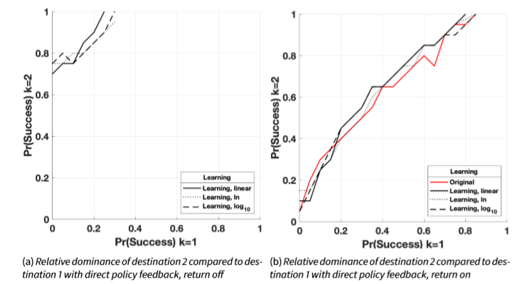
Figure 5a shows that this learning mechanism does not, in and of itself, produce spatial reorientation. It does not produce more spatial reorientation than what can be seen in Figure 2a. This test indicates that it is necessary for the size of the migrant stock to fluctuate across the two destinations for migration utility to change and reorientation to take place. Return migration is one such mechanism (see Section 5.3 in the body of the paper for a discussion of alternative mechanisms). Figure 5b shows a case where policy learning and return migration are both enabled to observe whether this type of learning may enhance spatial reorientation. Figure 5b also contains a red curve indicating the original model results. This figure shows that incorporating learning about immigration policy into agent decision-making has a minimal effect on overall results. This is likely because, in the original model, agents are already receiving signals about restrictive policy environments indirectly through a reduction in network size in a given destination, thereby affecting their utility to migrate. This means that agents will not attempt migration simply because their utility to migrate is low.
B: Results with larger sample size
The spatial division of the lattice and the number of agents are dependent upon each other, constraining the number of agents that could be used in the model. To satisfy the constraints of equations specified in the paper (see Equation 4 in particular), the following conditions must be met: 1) all locations must have the same number of cells, 2) no two agents can occupy a single cell, and 3) a single location must be able to house all agents, with no empty cells remaining. Netlogo’s square lattice always contains an odd number of cells, limiting our ability to divide it into equal quadrants with a neat number of cells in each.
In the model presented in the body of the paper, I initialized the model with 1,089 cells and assign one cell at coordinate (0,0) to be ‘no man’s land’. This left me with 1,088 cells that can be evenly split into quadrants of 272 cells each. In this paper, I only utilize three out of the four quadrants, with the fourth quadrant to be used for a three-destination extension to the model. To test the sensitivity of results to sample size, I run additional models with 8,930 agents. I initialize the model presented in this Appendix (Figure 6) with 35,721 cells and assign one cell at coordinate (0,0) to be dead space. This leaves me with 35,720 cells that can be evenly split into quadrants of 8,930 cells each.
The results shown in Figure 6 should be compared to Figure 2b in the body of the paper. In Figure 6, the values of \(Pr(Success) k=1\) and \(Pr(Success) k=2\) range from 0 to 1 with intervals of 0.2 (in Figure 2b intervals are 0.02) and models are run for 10 repetitions per parameter combination. Due to the large intervals used, the area where no migration takes place due to extreme policy restrictiveness in both locations (bottom-left corner), appears much larger than in Figure 2b. As can be observed in this figure, results are not significantly affected by number of agents.
C: Alternative network topology
In the main body I used a stylistic small world network topology. Although small world networks are commonly observed in a variety of systems, it is important to examine results using other network topologies. Random networks (Erdős 1959; Gilbert 1959) or regular networks (where each node connects to all of its nearest neighbors) are unlikely to be observed in real life (Barabási et al. 2016). However, comparing results under these different network topologies is important because it reveals the influence of network properties such as connectivity.
In all network configurations presented in this paper, the network is formed at initialization and agents begin a simulation run residing in their starting cell before the simulation run begins. An Erdös-Renyi (ER) network consists of a set of nodes, \(N\), where each node pair is connected with probability \({\pi}\). To construct the random network, I start with isolated agents and randomly select an agent pair and form a connection between the two with probability \({\pi}\). I repeat this step once for each possible agent pair. The degree distribution of a random network is binomial and varies depending on \(N\) and \(\pi\) (Barabási et al. 2016). In these tests, I set \(\pi\) to 0.022, such that agents have, on average, the same number of ties as in the body of the paper, \(\gamma = 6\), given the number of agents. Specifically, the model was run 100 times to examine variation in \(\gamma\), holding \(\pi\) at 0.022, and the average number of ties across all agents was computed. The average of this number over 100 runs is 5.98, with a standard deviation of 0.21 and a range of approximately 1.06. If \(\gamma \leq \ln(N)\), the graph is totally connected. This graph has the properties \(G(N=272, \pi=0.022)\) and, as such, has no isolated nodes.
To construct the regular network, each agent simply connects to its 6 nearest neighbors in a non-random fashion. A regular network is generally characterized by low connectivity or a long average path length. A long path length means that the average separation between individuals is much larger than the ER model. Because nodes are connected only to the nearest neighbors, these networks also display a high clustering coefficient compared to the ER model. As such, remote nodes may not be connected to one another. These characteristics make the transmission of information through a regular network less efficient. The small world network (Watts & Strogatz 1998) lies between the random network and the regular network. It displays a higher clustering coefficient than the ER model, but shorter average path lengths than a regular network. Small world networks are characterized by hubs, where information can be transferred efficiently to multiple nodes.
In Figure 7, I present the results for a random (blue), small world (red) and regular (cyan) network topology. In order to show all three results in the same graph, I display the policy area in which spatial reorientation takes place. This is comparable to the green area in Figure 2b. For these figures, I ran the model 100 times per setting and computed the average value of \(S_{t=24}\).
Results show there is very little difference between the random and small world networks implemented. However, results using a regular network show spatial reorientation occurring only when differences in policy restrictiveness between the traditional and alternative destination are very large. For instance, while spatial reorientation for the small world network setting occurs when \(Pr(Success) k=1\) is \(0.2\) and \(Pr(Success) k=2\) is \(\leq 0.4\), in the regular network setting, \(Pr(Success) k=2\) must be larger than \(0.7\) for reorientation to take place.
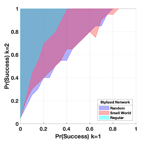
These results indicate that the efficient transmission of information among agents is important for spatial reorientation to take place. This is because, at first, only few individuals will migrate to the alternative location. For reorientation to take hold, these migrants must be able to communicate with agents in the origin country. If nodes are highly separated or not connected to one another, as we might expect in a regular network, the likelihood of this happening is lower. As such, for spatial reorientation to take place, the alternative destination must let in a larger number of individuals to compensate for the inefficient communication between nodes under a regular network topology.
Barriers in communication are an important line of inquiry in the study of migration, as distance or the conditions of travel (for example, amongst refugees) may make communication difficult. Further work should examine the relationship between communication barriers and the spatial distribution of migrants in more detail.
D: Number of ties
Figure 8 shows alternative results when agents have a median number of ties ranging from 4 – the median Mexican household size according to the MMP – to 10. I obtain the latter number of ties by adding all close and distant relationship variables available in the MMP dataset for each respondent and take the median of that value across the sample. Specifically, I add household members to all uncles, cousins, nephews, siblings-in-law, children-in-law, parents-in-law and friends who are currently in the US and those who have ever been in the US.
For these figures, I ran the model 100 times per each of the 7 degree settings and computed the average value of \(S_{t=24}\). Figure 8 displays the area where destination 2 is dominant or \(S_{t=24} > 0\). This is comparable to the green area of Figure 2b. In general, a higher number of ties make it less likely that destination 2 becomes dominant, although results are generally very similar within the range of 4 to 9 ties. We start to see a small reduction in the destination 2’s dominance area beginning to occur when the median number of ties is equal to 10. This is because a larger number of ties makes the system less sensitive to the migration of few individuals to the alternative destination. This, in turn, limits the rate of reorientation.
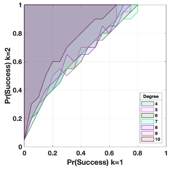
To understand why a reduction in destination 2’s dominance is taking place when agents’ have a large number of ties, it is useful to revisit Equation 6 in the body of the paper. Newcomers can derive benefits from migrants they are connected to through social ties and will therefore be drawn to the location where these migrants live. The network term \({N^k_i}\) is defined as the proportion of total network contacts living in destination \({k}\):
| $$N^k_i = \frac{|X^k_i|}{|X_i|}$$ | (16) |
As mentioned in Section 4.13, this lack of sensitivity should also affect the number of fluctuations in destination dominance observed over time. Figure 9 shows the average number of times, within a 24-year run, where the differences between the stock of migrants in destination 1 and destination 2 cross zero. Lighter tones signify a larger number of shifts in destination dominance. When comparing this figure to Figure 3, we can see that the maximum number of fluctuations that can occur across the parameter space is reduced from 7 to 5.72.
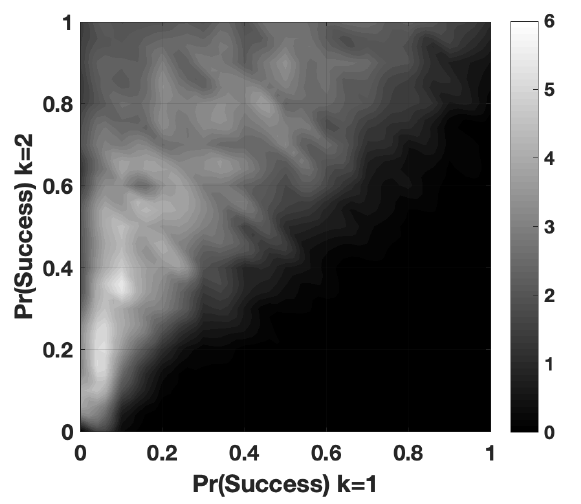
E: Strong and weak ties
The distinction between strong and weak ties has received attention in research on migrant networks. Social network theory expects that strong ties, such as close friends and family members, typically have stronger effects on migration facilitation than weak ties. This is because strong ties are able to provide “thick information and active assistance” (Garip & Asad 2016, p. 1171). However, Granovetter’s ‘strength of weak ties’ argument (1973) has had an important impact on how we conceptualize migrant networks, opening up a new, though relatively unexplored, area of research in migration networks (Collyer 2005; Boyd 1989; De Haas 2010). Granovetter argues that, while close contacts in a social network are likely to have very similar information, individuals are more likely to be able to obtain new information through a more distant, weaker, connection. In the present study, a weak network contact could provide information about the alternative destination and drive migration there.
Following Garip & Asad (2016), weak social network ties can be operationalized as network ties with whom agents are less likely to communicate. In these tests, I initialize the model with each agent having an average of 10 network ties and approximately 6 of these marked as strong ties (as in the body of the paper). The size of this extended network was determined using data from the MMP. As specified in Section 3.7, I consider strong ties to be blood relatives. Specifically, they consist of household members, uncles, cousins and nephews currently in Mexico. I compute the extended network by adding all network variables available in the MMP dataset and taking the median. This includes blood-related family ties currently in the US, siblings-in-law, children-in-law, parents-in-law and friends who are currently or have ever been in the US.
In the model, agents construct a ‘support network.’ Ties that are tagged as being part of an agent’s support network will provide information to the agent and, more generally, influence their utility for migrating to the destination where these ties are located in the manner described throughout this paper. All strong ties are automatically part of an agent’s support network. Weak ties have a 50 percent chance of being a member. Agents will not consider anyone outside their support network in any model process. Because I increase the size of the network rather than simply tagging nodes within the original \(\gamma= 6\) network as weak ties, I increase agents’ probability of obtaining new information from these additional network ties.
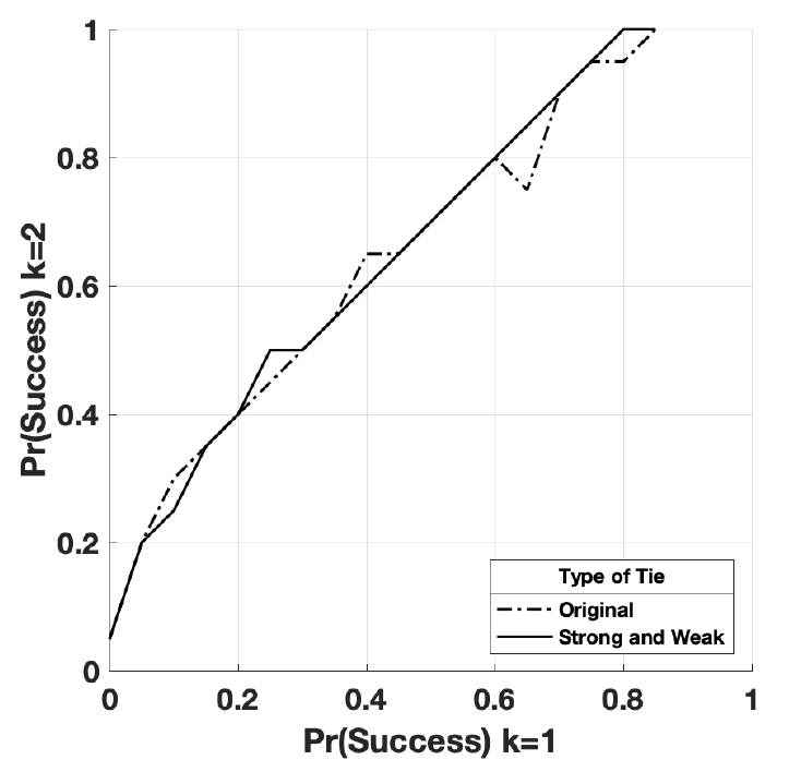
As Figure 10 shows, there is no significant difference between the original and the network-differentiated model. Further work should expand upon Granovetter’s predictions.
F: Alternative return equation parameters
Migrants’ utility for returning home was defined by Equation 11 in the main body. Return migration utility, \({U^r_i}\), is a function of the benefit of an additional network tie residing in the home country and the benefit of approaching savings target \({\eta}\). These are the first and second components, respectively, on the right hand side of the equation. As both components are necessary for return, utility is modeled multiplicatively:
| $$U^r_i = \frac{\log(aN^h_i + 1)}{\log(a + 1)} \Bigg(\frac{2}{1 + \exp(-bs^k_i)} - 1\Bigg)$$ | (17) |
\({N^h_i}\) is defined as the proportion of ties to individuals in migrants’ home location over their total number of connections. All else equal, the larger \({N_i^h}\), the larger the motivation to return.
To solve for constants a and b, I held the second utility component at the savings target, and found two values or ‘anchor points’ for the first utility component – network benefits – in terms of \({U^r_i}\). In the main results, when \({N_i^h = 1}\), I set \({U^r_i}\) to 0.9. I refer to this equation as the ‘high utility’ equation. When \({N_i^h = 0.3}\), \({U^r_i = 0.6}\), slightly above the midpoint. I refer to this equation as the ‘low utility’ equation. The constants resulting from solving these simultaneous equations are: \({a=28.4681}\) and \({b=0.0011}\). The function is shown in Figure 11.
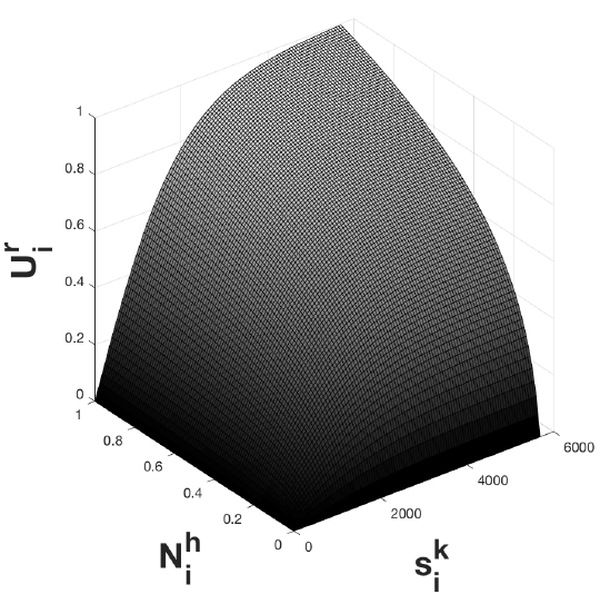
To test the sensitivity of the assumptions made above, I vary \({U^r_i}\) from 0 to its maximum value, 1, at intervals of 0.1, maintaining the values of \({N_i^h}\) and \(\eta\) the same as above. In these tests, the ‘high utility’ equation will, by definition, always have a strictly larger value of \({U^r_i}\) than the ‘low utility’ equation. For example, if \({U^r_i}\) for the ‘low utility’ equation is set to 0.5, \({U^r_i}\) for the ‘high utility’ equation can only vary between 0.6 and 1. Table 2 shows values of constants \(a\) and \(b\) for all equations that were solvable. Those that were not, are listed as ‘NA.’
| \(U^h_i\) hi/lo | 0.1 | 0.2 | 0.3 | 0.4 | 0.5 | 0.6 | 0.7 | 0.8 |
| 0.2 | \(a=4.44\) \(b=1\text{e-}4\) | |||||||
| 0.3 | \(a=0.36 b=2\text{e-}\) | \(a=28.47\) \(b=2\text{e-}4\) | ||||||
| 0.4 | \(a=-0.40\) \(b=3\text{e-}4\) | \(a=4.44\) \(b=3\text{e-}4\) | \(a=112.83\) \(b=3\text{e-}4\) | |||||
| 0.5 | NA | NA | NA | NA | ||||
| 0.6 | NA | \(a=0.36\) \(b=5\text{e-}4\) | \(a=4.44\) \(b=5\text{e-}4\) | \(a=28.47\) \(b=5\text{e-}4\) | NA | |||
| 0.7 | NA | NA | NA | NA | NA | NA | ||
| 0.8 | NA | \(a=-0.40\) \(b=8\text{e-}4\) | NA | \(a=4.44\) \(b=8\text{e-}4\) | NA | \(a=112.83\) \(b=8\text{e-}4\) | NA | |
| 0.9 | NA | NA | \(a=0.36\) \(b=1.1\text{e-}3\) | NA | NA | \(a=28.47\) \(b=1.1\text{e-}3\) | NA | NA |
First, I examine how these parameter settings affect the average length of stay of agents. I run 100 simulations for each of the 14 parameter combinations. Figure 12 displays the mean length of stay for a given constant (\(a/b\)) combination. Figure 12 shows results for four parameter combinations that are representative of the length of stay range for all 14 parameter combinations. For all figures, as policies for both destinations become more lax, the average length of stay abroad is longer for a given set of a/b parameter combination. This is because laxer policies allow for the accumulation of a larger network abroad, disincentivizing return. It also reduces migrants’ wages (see Equation 5), thereby increasing the time it takes agents to reach their savings target. Figure 12a shows the parameter settings used in the main results. For this figure, length of stay varies from 1.15 to 1.35 years across the full parameter range. Figures 12b to 12c also show negligible variation. Figure 12d displays much longer average length of stay values, ranging from 2 to 5.
However, despite the fact that length of stay does vary across settings, the main results remain fairly similar. In Figure 13, I reproduce the results obtained in Figure 2b for each of the \(a\) / \(b\) parameter combinations shown in Table 2. For each value of \(Pr(Success) k=1\), I compute the lowest possible value of \(Pr(Success) k=2\), for which \(S_t=24\) is larger than 0. I call this curve \(R\). The area above \(R\) covers the policy combinations at which destination 2 is dominant at the end of the simulation. I compute the average value of \(R\) across simulation runs for each of the 14 \(a\) / \(b\) parameter combinations. In Figure 13, I display the full range of \(R\), averaged within runs per \(a\) / \(b\) setting, as a gray ribbon. This figure shows that results does not appear to be substantially affected by the assumptions guiding the parametrization of the return utility equation.
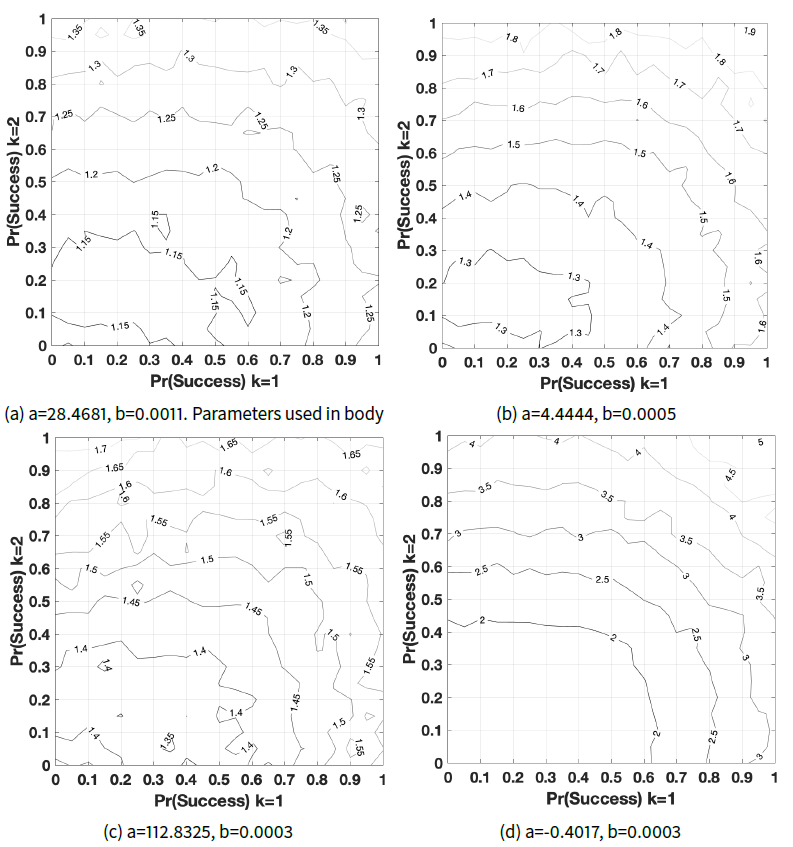
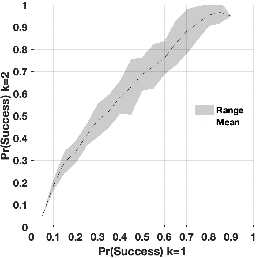
G: Likelihood of migrating among returnees
In the simple model presented in this paper, all agents have an equal chance of re-migrating. However, as (Massey & Zenteno 1999, p. 5328) explain, “once someone has lived and worked in a foreign setting, he or she is no longer the same person.” Working abroad changes personal motivations and attributes such that migrating again is more likely.
In this appendix, I examine the probability of re-migration as a function of past migratory experience. In these models, agents who have chosen to migrate attempt to do so with a probability \(p_x\), where \(x\) is the number of trips they have taken in the past. I operationalize past experience as a host country learning function. The more trips an individual makes, the more likely she is to re-migrate. I include three different functions for \(p_x\): a linear learning function, such that each additional trip taken has the same effect on the probability of re-migrating and two log functions (\(\ln\) and \(\log_{10}\)). For the log learning functions, each trip has a smaller marginal effect on overall learning (Estes 1950; Heathcote et al. 2000). The maximum value of \(x\) is equal to the maximum number of trips taken by agents, on average, under the most liberal policy conditions (both countries have open borders): 11.
Agents will make an initial trip with \(p_x = 1\), as in the original model. That is, if they have chosen a destination, they will attempt to migrate. Host country learning will only apply to migrations subsequent to the first. This is because, if the probability of attempting migration is a direct function of the number of previous trips, then the probability of attempting an initial trip would be 0 and we would not be able to observe re-migration at all.
Figure 14 shows the policy area where spatial reorientation takes place, allowing us to compare the effects of host country learning functions. For reference, the original configuration is shown in yellow. These tests show that reorientation is more likely when the probability of re-migrating is equal for all agents – the original model. This is because frequent return and re-migration helps change the spatial distribution of migrants. Reorientation is slightly more likely when the probability of attempting an additional trip rises quickly with few prior migration trips – the \(\log_{10}\) model.
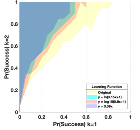
In future work, agents should acquire social and financial capital when migrating and these attributes should be reflected in countries’ policies. For example, agents can acquire skills that can make them eligible for a wider range of visas or valuable connections that can sponsor them (Simon et al. 2018).
References
ADAMS, R., Mora, J. & Taylor, J. E. (2005). Remittances, inequality and poverty: Evidence from rural Mexico. In American Agricultural Economics Association Annual Meeting.
AMUEDO-DORANTES, C. & Mazzolari, F. (2010). Remittances to Latin America from migrants in the United States: Assessing the impact of Amnesty programs. Journal of Development Economics, 91(2), 323–335.
ANGELUCCI, M., De Giorgi, G., Rangel, M. A. & Rasul, I. (2009). Extended family networks in rural Mexico: A descriptive analysis. IZA Discussion Paper No. 4498.
ARANGO, J. (2000). Explaining migration: A critical view. International Social Science Journal, 52(165), 283–296.
ARANGO, J. (2004). Theories of International Migration. In D. Joly (Ed.), International Migration and the New Millennium. Aldershot: Ashgate.
BALÁŽ, V., Williams, A. M. & Fifeková, E. (2014). Migration decision making as complex choice: eliciting decision weights under conditions of imperfect and complex information through experimental methods. Population, Space and Place, 22(1), 36–53.
BARABÁSI, A.-L. (2016). Network Science. Cambridge, NY: Cambridge University Press.
BARBOSA, Filho, H. S., de Lima Neto, F. B. & Fusco, W. (2011). Migration and social networks: An explanatory multi-evolutionary agent-based model. In 2011 IEEE Symposium on Intelligent Agent (IA), (pp. 11–15).
BIONDO, A. E., Pluchino, A. & Rapisarda, A. (2013). Return migration after brain drain: A simulation approach. Journal of Artificial Societies and Social Simulation,16(2), 11: https://www.jasss.org/16/2/11.html. [doi:10.18564/jasss.2161]
BOHN, S. & Pugatch, T. (2015). U.S. border enforcement and Mexican immigrant location choice. Demography, 52, 1543–1570.
BORJAS, G. J. (1995). The economic benefits from immigration. Journal of Economic Perspectives, 9(2), 3–22. [doi:10.1257/jep.9.2.3]
BOYD, M. (1989). Family and personal networks in international migration: Recent developments and new agendas. International Migration Review, 23(3), 638–670.
BRENNER, T. & Werker, C. (2009). Policy advice derived from simulation models. Journal of Artificial Societies and Social Simulation, 12(4), 2: https://www.jasss.org/12/4/2.html.
BRUCH, E. & Atwell, J. (2015). Agent-based models in empirical social research. Sociological Methods Research, 44(2), 186-221.
CARRINGTON, B. W. J., Detragiache, E. & Vishwanath, T. (1996). Migration with endogenous moving costs. American Economic Review, 86(4), 909–930.
CASTLES, S., Miller, M. J. & Ammendola, G. (2003). The Age of Migration: International Population Movements in the Modern World. The Guilford Press.
CEDERMAN, L. E. (1997). Emergent Actors in World Politics. New York: Princeton University Press.
CLEMENS, M., Huang, C., Graham, J. & Gough, K. (2018). Migration is what you make it. Technical Report. May.
COLLYER, M. (2005). When do social networks fail to explain migration? Accounting for the movement of Algerian asylum seekers to the UK. Journal of Ethnic and Migration Studies, 31(4), 699–718. [doi:10.1080/13691830500109852]
CONSTANT, A. & Massey, D. S. (2002). Return migration by German guestworkers: Neoclassical versus New Economic Theories. International Migration, 40(4), 5–38.
CONSTANT, A. F. & Zimmermann, K. F. (2012). The dynamics of repeat migration: A Markov chain analysis. International Migration Review, 46(2), 362–388. [doi:10.1111/j.1747-7379.2012.00890.x]
CZAIKA, M. & De Haas, H. (2014). The globalization of migration: Has the world become more migratory? International Migration Review, 48(2), 283–323.
DE HAAS, H. (2010). The internal dynamics of migration processes: A theoretical inquiry. Journal of Ethnic and Migration Studies, 36(10), 1587–1617. [doi:10.1080/1369183X.2010.489361]
DE HAAS, H. (2011). The determinants of international migration: conceptualizing policy, origin and destination effects. Working Paper 32, International Migration Institute.
DE HAAS, H. & Fokkema, T. (2011). The effects of integration and transnational ties on international return migration intentions. Demographic Research, 25(24), 755–782. [doi:10.4054/DemRes.2011.25.24]
DURAND, J., Massey, D. S. & Parrado, E. A. (1999). The new era of Mexican migration to the United States. The Journal of American History, 86(2), 518–536.
DUSTMANN, C. (2003). Return migration, wage differentials, and the optimal migration duration. European Economic Review, 47(2), 353–369. [doi:10.1016/S0014-2921(01)00184-2]
ELLIS, M., Wright, R., Townley, M. & Copeland, K. (2014). The migration response to the legal Arizona Workers Act. Political Geography, 42, 46–56.
ENTWISLE, B., Williams, N. E., Verdery, A. M., Rindfuss, R. R., Walsh, S. J., Malanson, G. P., Mucha, P. J., Frizzelle, B. G., McDaniel, P. M., Yao, X., Heumann, B. W., Prasartkul, P., Sawangdee, Y. & Jampaklay, A. (2016). Climate shocks and migration: an agent-based modeling approach. Population and Environment, 38(1), 47–71. [doi:10.1007/s11111-016-0254-y]
EPSTEIN, G. S. (2008). Herd and network effects in migration decision-making. Journal of Ethnic and Migration Studies, 34(4), 567–583.
EPSTEIN, J. M. (1999). Agent-based computational models and generative social science. Complexity, 4(5), 41–60. [doi:10.1002/(SICI)1099-0526(199905/06)4:5<41::AID-CPLX9>3.0.CO;2-F]
EPSTEIN, J. M. & Axtell, R. (1996). Growing Artificial Societies: Social Science from the Bottom Up. Washington, DC: Brookings Institution Press.
ERDŐS, A., P; Rényi (1959). On Random Graphs. Publicationes Mathematicae, 6, 290-297.
ESPINDOLA, A. L., Silveira, J. J. & Penna, T. J. P. (2006). A Harris-Todaro agent-based model to rural-urban migration. Brazilian Journal of Physics, 36(3A), 603–609.
ESTES, W. K. (1950). Toward a statistical theory of learning. Psychological Review, 57(2), 94. [doi:10.1037/h0058559]
FAGIOLO, G. & Mastrorillo, M. (2013). International migration network: Topology and modeling. Physical Review E, 88(1), 012812.
FAIST, T. (1997). 'The Crucial Meso Level.' In T. Hammar, G. Brochmann, K. Tamas & T. Faist (Eds.), International Migration, Immobility and Development: Multidisciplinary Perspectives. Oxford: Berg, pp. 187–217.
GARCÍA, Á., Griesbach, K., Andrade, J., Gonzalez, C., Barbosa, G. Y., Alarcón, R. & Muse-Orlino , L. (2011). Pressure from the inside: The subnational politics of immigration. In R. A. y. L. M.-O. David Fitzgerald (Eds.), Recession without Borders, Mexican Migrants Confront the Economic Downturn, Center for Comparative Immigrations Studies, University of California, San Diego.
GARCÍA-DÍAZ, C. & Moreno-Monroy, A. I. (2012). Social influence, agent heterogeneity and the emergence of the urban informal sector. Physica A: Statistical Mechanics and its Applications, 391(4), 1563–1574. [doi:10.1016/j.physa.2011.08.057]
GARIP, F. & Asad, A. L. (2016). Network effects in Mexico–US migration: disentangling the underlying social mechanisms. American Behavioral Scientist, 60(10), 1168–1193.
GILBERT, E. N. (1959). Random graphs. The Annals of Mathematical Statistics, 30(4), 1141–1144. [doi:10.1214/aoms/1177706098]
GILBERT, N. (2008). Agent-based models. Series No 153. California: Sage.
GILBERT, N., Ahrweiler, P., Barbrook-Johnson, P., Narasimhan, K. P. & Wilkinson, H. (2018). Computational modelling of public policy: Reflections on practice. Journal of Artificial Societies and Social Simulation, 21(1), 14: https://www.jasss.org/21/1/14.html. [doi:10.18564/jasss.3669] <
GLENNIE, A. & Chappell, L. (2010). Jamaica: from diverse beginning to diaspora in the developed world. Migration Policy Institute: http://www.migrationpolicy.org.
GONZÁLEZ-BARRERA, A. (2015). More Mexicans leaving than coming to the US. Pew Research Center, 19.
GRANOVETTER, M. S. (1973). The strength of weak ties. American Journal of Sociology, 78(6), 1360–1380.
GUARNIZO, L. E., Portes, A. & Haller, W. (2003). Assimilation and transnationalism: Determinants of transnational political action among contemporary migrants. American Journal of Sociology, 108(6), 1211. [doi:10.1086/375195]
GURAK, D. T. & Caces, F. (1992). Migration networks and the shaping of migration systems. In M. M. Kritz, L. L. Lim & H. Zlotnik (Eds.). International Migration Systems: A Global Approach (pp. 150-176). Oxford, England: Clarendon Press: http://www.popline.org/node/319820
HARRIS, J. R. & Todaro, M. P. (1970). Migration, unemployment and development: A two-sector analysis. The American Economic Review, 60(1), 126–142.
HASSANI-MAHMOOEI, B. & Parris, B. W. (2012). Climate change and internal migration patterns in Bangladesh: An agent-based model. Environment and Development Economics, 17, 763–780.
HATTLE, A., Yang, K. S. & Zeng, S. (2016). Modeling the Syrian refugee crisis with agents and systems. UMAP Journal, 37(2). [doi:10.1080/13691830801961605]
HATTON, T. J., & Williamson, J. G. (1998). The Age of Mass Migration: Causes and Economic Impact. Oxford: Oxford University Press.
HAUG, S. (2008). Migration networks and migration decision-making. Journal of Ethnic and Migration Studies, 34(4), 585–605.
HEATHCOTE, A., Brown, S. & Mewhort, D. (2000). The power law repealed: The case for an exponential law of practice. Psychonomic Bulletin & Review, 7(2), 185–207.
HEILAND, F. (2003). 'The collapse of the Berlin wall: Simulating state-level East to West German migration patterns.' In F. C. Billari, F. Ongaro & A. Prskawetz (Eds.), Agent-Based Computational Demography: Using Simulation to Improve Our Understanding of Demographic Behaviour (Vol. IX, p. 210). Elsevier. [doi:10.1007/978-3-7908-2715-6_5]
HOLLIFIELD, J., Martin, P. & Orrenius, P. (Eds.). (2014). Controlling Immigration: A Global Perspective (Third Edition). Palo Alto, CA: Stanford University Press.
HOLLIFIELD, J. F. & Wong, T. K. (2000). 'The politics of international migration: How can we "Bring the State back In"?' In C. B. Brettell & J. F. Hollifield (Eds.), Migration Theory: Talking Across the Disciplines. London: Routledge.
JOHNSON, D. D., Weidmann, N. B. & Cederman, L. E. (2011). Fortune favours the bold: An agent-based model reveals adaptive advantages of overconfidence in war. PLoS ONE, 6(6), e20851.
JOHNSON, S. D. & Groff, E. R. (2014). Strengthening Theoretical Testing in Criminology Using Agent-Based Modeling. Journal of Research in Crime and Delinquency, 51(4), 509–525. [doi:10.1177/0022427814531490]
KING, R. (2012). Theories and typologies of migration : An overview and a primer, Willy Brandt Series of Working Papers in International Migration and Ethnic Relations, Willy Brandt Series of Working Papers Editor.
KLABUNDE, A. (2011). What explains observed patterns or circular migration? An agent-based model: http://andromeda.rutgers.edu/~jmbarr/EEA2011/klabunde.pdf [doi:10.1007/s10680-015-9362-0]
KLABUNDE, A. (2014). Computational economic modeling of migration. mimeo. Ruhr Universität.
KLABUNDE, A. & Willekens, F. (2016). Decision-making in agent-based models of migration: State of the art and challenges. European Journal of Population, 32(1), 73–97.
KLABUNDE, A., Zinn, S., Willekens, F. & Leuchter, M. (2017). Multistate modelling extended by behavioural rules: An application to migration. Population Studies, 71(1), 51–67.
KNIVETON, D., Smith, C. & Wood, S. (2011). Agent-based model simulations of future changes in migration flows for Burkina Faso. Global Environmental Change, 21. [doi:10.1016/j.gloenvcha.2011.09.006]
KNIVETON, D. R., Smith, C. D. & Black, R. (2012). Emerging migration flows in a changing climate in dryland Africa. Nature Climate Change, 2(6), 444–447.
KORINEK, K., Entwisle, B. & Jampaklay, A. (2005). Through thick and thin: Layers of social ties and urban settlement among Thai migrants. American Sociological Review, 70(5), 779–800. [doi:10.1177/000312240507000503]
KULU, H. & Milewski, N. (2007). Family change and migration in the life course: An introduction. Demographic Research, 17, 567.
LEACH, M. A. & Bean, F. D. (2008). The structure and dynamics of Mexican migration to new destinations in the United States. In New Faces in New Places: The Changing Geography of American Immigration, (pp. 51–74). Russell Sage Foundation New York.
LEE, E. S. (1966). A theory of migration. Demography, 3(1), 47–57.
LIANG, Z., Chunyu, M. D., Zhuang, G. & Ye, W. (2008). Cumulative causation, market transition, and emigration from China. American Journal of Sociology, 114(3), 706–737. [doi:10.1526/003601106777789828]
LICHTER, D. T. & Johnson, K. M. (2006). Emerging rural settlement patterns and the geographic redistribution of America’s new immigrants. Rural Sociology, 71(1), 109–131. [doi:10.1086/592860]
LICHTER, D. T. & Johnson, K. M. (2009). Immigrant gateways and Hispanic migration to new destinations. International Migration Review, 43(3), 496–518.
LIGHT, I., Bhachu, P. & Karageorgis, S. (1993). Migration networks and immigrant entrepreneurship. Immigration and Entrepreneurship: Culture, Capital, and Ethnic Networks, (pp. 25–50).
MA, Y., Shen, Z. & Kawakami, M. (2013). Agent-based simulation of residential promoting policy effects on down-town revitalization. Journal of Artificial Societies and Social Simulation, 16(2), 2.
MACDONALD, J. S. & MacDonald, L. D. (1964). Chain migration ethnic neighborhood formation and social networks. The Milbank Memorial Fund Quarterly, 42(1), 82–97. [doi:10.2307/3348581]
MASSEY, D., Goldring, L. & Durand, J. (1994a). Continuities in transnational migration: An analysis of nineteen Mexican communities. American Journal of Sociology, 99(6), 1492–1533.
MASSEY, D. S. (1999). International migration at the dawn of the Twenty-First Century: The role of the state. Population and Development Review, 25(1), 303–322. [doi:10.1111/j.1728-4457.1999.00303.x]
MASSEY, D. S., Alarcón, R., Durand, J. & González, H. (1987). Return to Aztlan: The Social Process of International Migration from Western Mexico. Berkley, CA: University of California Press.
MASSEY, D. S., Arango, J., Hugo, G., Kouaouci, A., Pellegrino, A. & Taylor, J. E. (1993). Theories of international migration: A review and appraisal. Population and Development Review, 19(3). [doi:10.2307/2938462]
MASSEY, D. S., Arango, J., Hugo, G., Kouaouci, A., Pellegrino, A. & Taylor, J. E. (1994b). An evaluation of international migration theory: The North American case. Population and Development Review, 20(4), 699–751.
MASSEY, D. S., Arango, J., Hugo, G., Kouaouci, A., Pellegrino, A. & Taylor, J. E. (1998). Worlds in Motion: Understanding International Migration at the End of the Millennium. Oxford: Clarendon Press.
MASSEY, D. S., Durand, J. & Pren, K. A. (2016). Why border enforcement backfired. American Journal of Sociology, 121(5), 1557–1600.
MASSEY, D. S. & Espinosa, K. E. (1997). What’s driving Mexico-US migration? A theoretical, empirical, and policy analysis. American Journal of Sociology, 102(4). [doi:10.1086/231037]
MASSEY, D. S. & Parrado, E. (1994). Migradollars: The remittances and savings of Mexican migrants to the USA. Population Research and Policy Review, 13(1), 3–30.
MASSEY, D. S. & Zenteno, R. M. (1999). The dynamics of mass migration. Proceedings of the National Academy of Sciences, 96(9), 5328–5335. [doi:10.1073/pnas.96.9.5328]
MEXICANS AND AMERICANS THINKING TOGETHER. (2013). The U.S./Mexico cycle: The end of an era. URL http://www.matt.org/.
MORETTI, E. (1999). Social networks and migrations: Italy 1876–1913. International Migration Review, 33(3), 640– 657.
MULDER, C. H. (1993). Migration dynamics: a life course approach. Amsterdam Netherlands Thesis Publishers.
MULDER, C. H. & Wagner, M. (1993). Migration and marriage in the life course: a method for studying synchronized events. European Journal of Population/Revue européenne de Démographie, 9(1), 55–76. [doi:10.1007/BF01267901]
OECD. (2009). Applications of Complexity Science for Public Policy: New Tools for Finding Unanticipated Consequences and Unrealized Opportunities. http://www.oecd.org/dataoecd/44/41/43891980.pdf
OECD. (2017). Perspectives on Global Development 2017: International Migration in a Shifting World. Organisation for Economic Cooperation and Development.
PALLONI, A., Massey, D. S., Ceballos, M. & Espinosa, K. (2011). Social capital and international migration: A test using information on family networks. American Journal of Sociology, 106(5), 1262–1298.
REHM, M. (2012). Migration and remittances. An agent-based model. Ph.D. thesis, New School University.
ROBERTS, K. D. & Morris, M. D. (2003). Fortune, risk, and remittances: An application of option theory to participation in village-based migration networks1. International Migration Review, 37(4), 1252–1281.
ROSSI, P. (1955). Why Families Move. New York: The Free Press.
SCHERER, S., Wimmer, M., Lotzmann, U., Moss, S. & Pinotti, D. (2015). Evidence based and conceptual model driven approach for agent-based policy modelling. Journal of Artificial Societies and Social Simulation, 18(3), 14. [doi:10.18564/jasss.2834]
SILVEIRA, J. J., Espindola, A. L. & Penna, T. J. P. (2006). Agent-Based model to rural-urban migration analysis. Physica A: Statistical Mechanics and its Applications, 64, 445–456. [doi:10.1016/j.physa.2005.08.055]
SIMON, M. (2019). The effects of immigration policy on migration systems. Ph.D. thesis, University College London.
SIMON, M., Schwartz, C., Hudson, D. & Johnson, S. D. (2018). A data-driven computational model on the effects of immigration policies. Proceedings of the National Academy of Sciences of the United States of America, 115(34). [doi:10.1073/pnas.1800373115]
SJAASTAD, L. A. (1962). The costs and returns of migration. Journal of Political Economy, 70(5), 80–93.
SMITH, C. D. (2014). Modelling migration futures: development and testing of the rainfalls agent-based migration model–Tanzania. Climate and Development, 6(1), 77–91. [doi:10.1080/17565529.2013.872593]
STARK, O., Helmenstein, C. & Yegorov, Y. (1997). Migrants’ savings, purchasing power parity, and the optimal duration of migration. International Tax and Public Finance, 4(3), 307-327.
SULEIMENOVA, D., Bell, D. & Groen, D. (2017). A generalized simulation development approach for predicting refugee destinations. Scientific Reports, 7(1), 13377. [doi:10.1038/s41598-017-13828-9]
TELESFORD, Q. K., Joyce, K. E., Hayasaka, S., Burdette, J. H. & Laurienti, P. J. (2011). The ubiquity of small-world networks. Brain connectivity, 1(5), 367–375.
TERRAZAS, A. (2011). Immigrants in new-destination states. Migration Policy Institutehttp://www.migrationpolicy.org/article/immigrants-new-destination-states.
U.S. DEPARTMENT OF STATE. (2015). Employment-based immigrant visas. http://travel.state.gov/visa/immigrants/types/types\_1323.html#first.
U.S. BUREAU OF LABOR STATISTICS. (2012). Consumer Price Index. Washington, DC.
U.S. CENSUS BUREAU (1993). We the American... Hispanics. Tech. Rep. September, U.S. Department of Commerce Economics and Statistics Administration.
WATTS, D. J. & Strogatz, S. H. (1998). Collective dynamics of small-world networks. Nature, 393(6684), 440–442. [doi:10.1038/30918]
WERTH, B. & Moss, S. (2007). Modelling migration in the Sahel: An alternative to cost-benefit analysis. In Takahashi, S., Sallach, D. & Rouchier, R." (Eds.). Advancing Social Simulation: The First World Congress, Springer (pp. 331–342).
WILENSKY, U. (1999). NetLogo. http://ccl.northwestern.edu/netlogo/
WILENSKY, U. (2005). NetLogo Small Worlds Model. http://ccl.northwestern.edu/netlogo/models/ SmallWorlds.
WILLEKENS, F. (2011). Migration: A Perspective from Complexity Science: New Approaches for Researching the Determinants of Migration Processes. ESF strategic workshop on migration research. University of Oxford: International Migration Institute and European Science Foundation.
WORLD BANK. (2018). Migration and remittances data. http://www.worldbank.org/ en/topic/migrationremittancesdiasporaissues/brief/migration-remittances-data (accessed 09-27-2018).
WOUTERSE, F. & Taylor, J. E. (2008). Migration and income diversification: Evidence from Burkina Faso. World Development, 36(4), 625–640. [doi:10.1016/j.worlddev.2007.03.009]
ZOLBERG, A. R. (1989). The next waves: migration theory for a changing world. International Migration Review, 23(3), 403–430.