Endogenous Changes in Public Opinion Dynamics

Introduction

Opinions are a relevant ingredient in the explanation of social behavior, and public opinion dynamics should be a relevant ingredient in the explanation of social regularities and social change. In addition, public opinion is sometimes considered a key in shaping political decisions and, therefore, in the design of our institutions and public policies (for some reviews on the topic see, for example, Burstein 2003; Manza et al. 2002; Wlezien and Soroka 2007).

For all these reasons, public opinion has been one of the classical objects of study in sociology. Social science is leaving the traditional descriptive approach behind and is now turning to the construction of generative models that allow us to better understand how and why opinions change as a result of personal experiences, individual cognitive processes and social interaction. Sociophysics has taken the lead of this new causal and generative agenda and is currently offering opinion dynamics models at an overwhelming pace (for some reviews on sociophysic models see, for example, Castellano et al. 2009; Galam 2008; Lorenz 2007; Sîrbu et al. 2017). It is no surprise that mathematicians, computer scientists and physicists have turned their attention to this issue. Their tools not only seem to be useful for causally explaining opinion dynamics, but they have also found a crucial issue left unexplored by traditional social scientists.

To the best of our knowledge, however, there is an important limitation of sociophysic models that has not been addressed so far. A review of statistical physics models of opinion dynamics clearly shows a bias in their focus. The general idea of explaining macroscopic phenomena as the effect of interacting microscopic entities seems to have been interpreted in a very limited way, merely as a concern in the explanation of the emergence of regularities. Reflecting this bias, these opinion dynamics models usually describe how interactions bring about order out of disorder; consensus, polarization or fragmentation out of randomness (for a review, see Castellano et al. 2009; Sîrbu et al. 2017). But what about change? While the main concern of opinion dynamics models seems to be whether the initial disorder generates uniformity, clusterization or polarization, other interesting and relevant social dynamics, such as the process behind slow changes, equilibrium shifts or abrupt fluctuations, are less understood. The study of changes in public opinion regularities is generally dismissed in sociophysic models (some exceptions are Acemoğlu et al. 2013; Galam 1986, 1990, 1999, 2000), as if changes in macro-regularities would not also be macro-phenomena to be explained as the effect of microscopic interactions. But they are. In fact, these changes are relevant features of natural opinion dynamics without which we cannot achieve a truly and comprehensive understanding of this phenomenon.

Outside the field of sociophysics, the classical work of Timur Kuran (1987a, 1987b, 1989, 1990, 1991a, 1991b, Kuran 1995) highlighted preference falsification as one of the possible mechanisms behind abrupt changes in public opinion that seem to explain unexpected revolutions. But we do not know much about other possible mechanisms that could explain these and other types of shifts in public opinion.

This is a serious gap in our knowledge of public opinion. Public opinion is not static; it undergoes all kinds of changes. The variety of those changes is so huge that we need some classification of types to cope with the phenomenon. Since constructing a typology of changes in public opinion is not the goal of this paper, we just assume a quite simple typology based on how radical the change is and how rapid it unfolds. An illustration of the four types of changes in this typology is shown in Figure 1.

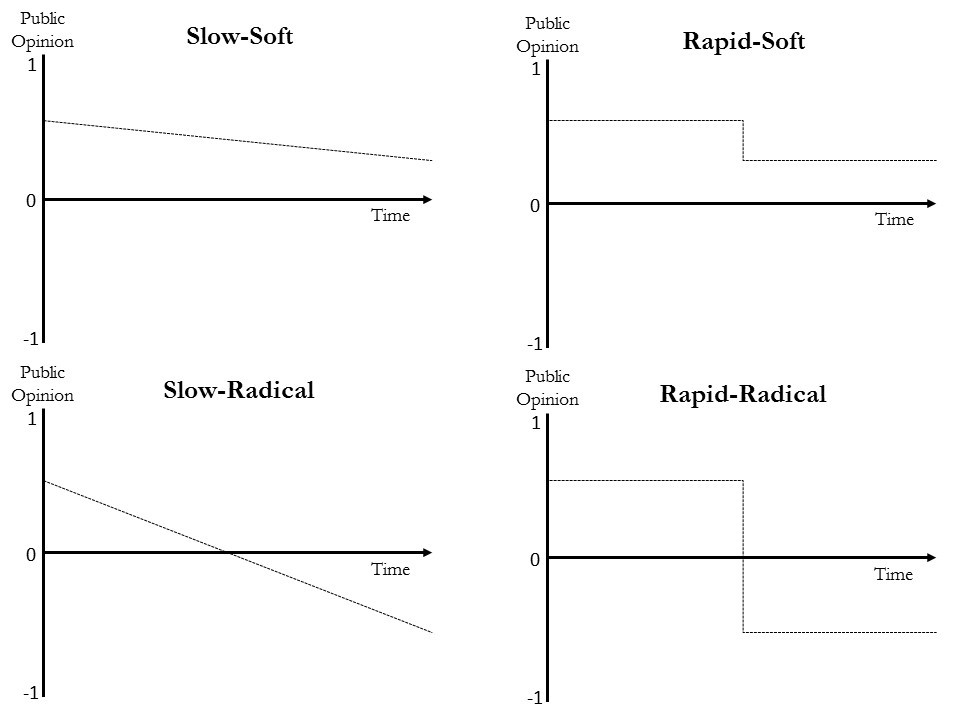
According to our typology, public opinion sometimes slowly experiences a radical change that is almost unperceived in the short term (a slow-radical change); it sometimes experiences a soft change that takes a long period of time to unfold (a slow-soft change); public opinion sometimes changes moderately but in a very short period of time (a rapid-soft change); and sometimes it radically changes in an abrupt way (a rapid-radical change). But what we do know about the microfoundations of those changes?

Our goal was to build a multi-agent model whose dynamics were, at least under certain conditions, characterized by different types of endogenously (that is, not induced by the researcher) triggered changes: constant and moderate fluctuations, radical changes after long periods of stability, slow transitions, etc. If our model could show this kind of behavior, then we could unravel the generative processes behind those changes, therefore adding new candidates to the set of causal hypotheses to be considered when tackling the explanation of natural changes in public opinion.

This paper is organized as follows. First, we present the model, specifying the algorithms for network constructions and the formalization of the different cognitive and social interaction mechanisms behind the actualization of opinions at the individual level. Second, we present some results of the model in a descriptive way, showing how the output and dynamics of the model vary depending on its initial conditions. Third, we try to shed light on the micro-level generative process that explains these outputs. The last section concludes.

The Model

Network formation

We have run our model^[1] in three different network structures to test if these topographies have a role in the generation of different public opinion dynamics. Before running the model, we trigger a network morphogenesis that generates either a random, a small-world or a scale-free network. To make these different network structures comparable, we kept the number of agents and links constant: all networks have 500 nodes and \(\approx\)1000 undirected links, that is, \(k_i \approx 4\), where \(k_i\) refers to the mean degrees of all nodes, that is, the mean size of all agents’ neighborhoods.

Random network. According to the \(G(n,p\) variant of the Erdős–Rényi model (Erdös and Rényi 1959), the algorithm that we used to generate random networks (RNs hereafter) is as follows:

1. A set of 500 disconnected nodes is created.
2. Every pair of nodes is connected with a probability of \(p\).
3. Since the number of expected edges is \(E(n) = p \Bigl[ \frac{n ( n - 1 )}{2}\Bigr]\), and considering that we want 500 nodes and \(\approx\)1000 edges, \(p\) is set to 0.008.

Small-world network. We used the Watts-Strogatz model (Watts and Strogatz 1998) to generate small-world networks (SWNs hereafter). The algorithm of this model is as follows:

1. A set of 500 nodes is created forming a ring.
2. Each node is connected to its 2 nearest neighbors to the left and its 2 nearest neighbors to the right, so we obtain a network with 1000 undirected links.
3. Each edge is randomly rewired with probability \(p\) (self-connections and duplicate edges are excluded). We set \(p = 0.5\).^[2]

Scale-free network. To generate scale-free networks (SFNs hereafter) our algorithm is based on the Barabási Albert model (Barabási and Albert 1999):

1. A set of 5 nodes is created in a fully connected network.
2. A new node is created. This new node chooses two pre-existing nodes to connect with using a roulette-wheel selection process based on agents’ probabilities of being selected. These probabilities are determined by a preferential attachment mechanism: a fitness function that depends on the degree of each existing node (\(k\)) represents its probability of being chosen. Specifically, the probability of a node \(i\) being chosen is equal to \(i\)’s degree over the sum of all the degrees of the already existing nodes.
3. Step b) is repeated 495 times to get a \(n = 500\). The preferential attachment mechanism represents the situation where more connected nodes are more likely to attract new connections. The result is a scale-free network with a power-law degree distribution.

Opinion dynamics

In this model, opinion expression is the result of several cognitive and social mechanisms: a coherence mechanism, in which agents try to stick to their previously expressed opinions, an assessment mechanism, in which agents consider the available external information regarding the issue at hand, and a social influence mechanism, in which agents tend to approach their neighbor’s opinions.

One of the traditional critiques of sociophysic models is that they achieve parsimony by means of an excessive unrealism of the assumptions (see, for example, Duggins 2017: 1.2; Moussaïd et al. 2013: 1 and Sobkowicz 2009). As we see it, opinion dynamics models, as any other type of models, should find a balance between realism and simplicity, at least if they are built for explanatory purposes. We have included these three mechanisms because, as we shall see below, there is empirical evidence of their relevance in processes of opinion formation, change and exchange. Modeling these three mechanisms generates a model that is not as parsimonious as some traditional sociophysics models, but a more realistic yet analyzable one.

Our model is a continuous opinion model in which agents express a public opinion in the interval \([-1,1]\). Initially, each agent is given an opinion which is randomly chosen from a uniform distribution, but the opinion they express in each time-step of the simulation is the result of a declaration process that unfolds in two steps.

First step

First, agents establish their provisional opinion (\(x'_i\)):

$$x'_i = c_i + \mu (a_i - c_i)$$

(1)

This provisional opinion is composed of two elements:

The coherence element (\(c_i\)). This element refers to the constant actualization of our private beliefs and is defined here as the mean of the three last opinions that agent \(i\) expressed in public. In the absence of other influences, this element determines the opinion that \(i\) will express. Traditional models on opinion dynamics, like the family of Bounded Confidence Models that include the Deffuant or Deffuant-Weisbuch model (Deffuant et al. 2000; Weisbuch et al. 2002, Weisbuch et al. 2003) and the Hegselmann-Krause model (Krause 2000; Hegselmann & Krause 2002) usually consider individuals’ opinions as the output of a social exchange of prior opinions. However, as stated by Wang, Huang, & Sun (2013), in opinion formation and evolution, individuals also deal with their self-attitudes and, as self-perception theory posits (Bem 1972), we frequently come to clarify our attitude (or private opinion) through observing our own behavior (or public opinion). If, as a consequence of a social exchange of opinions, an individual expresses certain opinions regarding the issue \(x\) that were at odds with his private ones, this behavior will eventually affect his inner attitude regarding \(x\). A plausible mechanism to explain this adjustment of private opinion is the drive to reduce cognitive dissonance (Festinger 1957): the dissonance produced by conflicting private and public opinions is likely to be suppressed by aligning the private opinion to the publicly expressed one, and not the other way around. At the same time, it is plausible to assume that people tend to stick to their previously expressed opinions: we all try to keep a certain stability in the opinions that we express in public regarding a specific topic. This is known as behavioral consistency (Cialdini 2009). As stated by Cialdini, we all try to show behaviors that are consistent with our own past behaviors. Behavioral inconsistency is seen as an undesirable individual trait, so avoiding the individual and social pressures that apply when inconsistency is perceived can be the reason why people actualize their private opinions to match their previously expressed ones.

The assessment element (\(a_i\)). Following the tradition of exploring the role of external information in opinion dynamics, our model introduces signals which represent the opinions the agent gets from external sources, like media or experts, not from the agent’s interactions with neighbors. In most opinion dynamics models that have studied the effect of mass media, the external information either takes a constant value or changes at each time step. This is the case of models like those of Carletti et al. (2006), Crokidakis (2012), Gargiulo et al. (2008), González-Avella et al. (2012), Laguna et al. (2013) and Martins et al. (2010). However, in all these cases, the external information is the same for all agents. Few models capture multiple mass media sources (one of them is Quattrociocchi et al. 2014). We try to go a step further, considering external sources of information that vary from agent to agent. In each time-step, each agent gets a signal related to the issue to which the opinion refers and considers \(a_i\) the mean of his last three signals.

Since signals are nothing but opinions that agents get from external sources, they have values in \([-1,1]\). The value of signals is experimentally manipulated, so it can be randomly chosen for each agent in each time-step from a uniform distribution, from a normal distribution with a mean value equal for all agents, or from a normal distribution with a mean that depends on the opinion of each agent. A uniform distribution would represent the unusual situation where signals are completely random. A normal distribution could represent a situation where the external source basically transmits signals around a certain opinion, as usually happens when media are controlled by government, or when experts talk about a non-controversial issue. Finally, a normal distribution with a mean that depends on each agent’s opinion could be useful to represent different people getting signals from different media depending on their ideological closeness. In our case, for example, agents with \(x \geq 0\) (we shall call them right-wingers) get a signal randomly chosen from a normal distribution with mean 0.5, while agents with \(x < 0\) (left-wingers) get a signal randomly chosen from a normal distribution with mean −0.5 (in both cases we set SD \(=\) 0.35)^[3]. What we are trying to model here is the commonly known fact that people usually get signals that are generally in line with their opinion, that is, people get structured, non-random signals. Left-wingers usually read left-wing newspapers, for example. In these newspapers, signals are diverse: there are different opinions on the same subject in opinion articles and editorials, some of which can even be considered right-wing, but this diversity revolves around a left-wing editorial policy. The same is true for right-wingers and the signals that they get from right-wing newspapers. It is also plausible to assume that when right-wingers (left-wingers) change their mind and become left-wingers (right-wingers), they also change their habitual source of information (their preferred newspaper, for example).

The parameter \(\mu\) fine tunes the degree to which the provisional opinion is affected by the assessment, obviously including the possibility that an agent is completely impermeable to any evidence or information against his opinion.

Second step

In the second step, the opinion that agents will publicly express (\(x_i\)) is affected by a social influence mechanism, which refers to the effect of their neighbors’ opinion on their own opinion. In this case, we formalize a positive social influence mechanism, that is, a conformity mechanism that reflects the tendency to reduce the opinion distance with peers.

$$x_i = x'_i + \theta_i (r_i - x'_i)$$

(2)

In this model, each agent considers his own reference opinion (\(r_i\)). This reference opinion is almost identical to the update rule for the opinion of an agent in a Hegselmann-Krause model (2002), but here an agent does not consider the average opinion of his neighbors but the weighted arithmetic mean of the public opinions of his neighbors. Opinions are weighted depending on the degree of each node, therefore capturing the fact that more connected nodes have more influential opinions. In our model, persuasiveness (the ability to make others change their opinion) and supportiveness (the capacity to reinforce others’ opinions), as defined by the psychological theory of social impact (Latané 1981), are assumed to be higher in highly connected nodes.

$$r_i = \frac{\sum (k_z \ast x_z)}{\sum k_z}$$

(3)

Where \(z\) refers to any agent that is connected with \(i\) and, therefore, \(k_z\) refers to \(z\)’s node degree and \(x_z\) refers to \(z\)’s opinion.

\(\theta_i\) captures how much this difference affects the individual, that is, it captures \(i\)’s susceptibility to social influence. This parameter is equivalent to the convergence parameter of the Deffuant model (Deffuant et al. 2000). In fact, the general idea behind equation 2 is equivalent to that of the Deffuant model, but in our case, \(i\) considers his provisional opinion and approaches it to the weighted arithmetic mean of the public opinions of his neighbors. Regarding \(\theta_i\), it is plausible to assume that this susceptibility is a function of the node degree: more connected nodes are assumed to be influencers and less connected nodes are assumed to be the object of that influence. Therefore we just assumed \(\theta_i\) as perfectly correlated with \(k_i\) and rescaled to \([0,1]\). As can be seen, there are no zealots in this model and therefore anyone can end up changing his opinion, but highly connected agents are assumed to be more committed to their opinions.

In order to moderate the impact of social influence, we assume that in the highest degree of influence the agent moves his opinion to the intermediate point between his provisional opinion and his reference opinion:

$$\theta_i = \frac{1}{2} \Biggl( 1 + \frac{-k_i + \min (k)}{\max (k) - \min (k)} \Biggr)$$

(4)

This moderate impact of social influence reflects the empirical finding of Moussaïd et al. (2013), who experimentally showed that there is a bias toward one’s initial opinion when exposed to other’s different opinions and even when the agent compromises, the opinion change is only limited.

Output

Public opinion is defined here as the mean of individual opinions at each moment of time. Therefore, the evolution of the mean of individual opinions and the shape of this distribution shall be the main output to be analyzed.

In sum, in our model:

1. Each simulation takes place in a different network structure: either a random, a small-world or a scale-free network.
2. Agents try to be coherent with their previously expressed opinions.
3. Agents get external signals that may change their opinion depending on their level of resistance or impermeability.
4. Agents approach their opinion to the opinion of their neighborhood but consider the opinion of more connected neighbors as more valuable.
5. This approach to the opinion of the group depends on the agent’s susceptibility to social influence, and this susceptibility is a function of its degree.

Table 1: List of model variables (\(^\ast\)) The homophily parameter is introduced in a later section of the paper

Symbol	Variable
\(k_i\)	Node degree of agent \(i\)
\(x'_i\)	Provisional opinion of agent \(i\)
\(c_i\)	Coherence element
\(a_i\)	Assessment element
\(\mu\)	Relevance of \(a_i\) on \(x'_i\)
\(x_i\)	Opinion of agent \(i\)
\(r_i\)	Reference opinion of agent \(i\)
\(\theta_i\)	Susceptibility to social influence of agent \(i\)
\(h\)	Homophily (*)

Analysis

This section is divided in two parts. First, we test how the combination of type of network (random, small-world and scale-free) and level of subjective relevance of the assessment element (\(\mu\)) (values 0.2, 0.4, 0.6 and 0.8) affects opinion dynamics. This is a descriptive section. We will try to answer the following questions: does the system eventually reach some stable state in \(\bar{x}_i\)? Does the system occasionally experience a transition from one steady state to another? When those transitions occur, do their type, frequency and structure vary depending on the type of network and the level of \(\mu\)? In addition, we explore the effect of homophily in public opinion transitions. The second part is devoted to explaining the patterns described in the first section. Therefore, in the second part, we shall focus on unraveling the generative process behind those patterns.

The role of networks and external information

Opinion dynamics in this model are highly dependent on the type of distribution from which agents get the signals that they use to form their assessment element (\(a_i\)). Recall here that these signals represent any kind of information and opinions regarding the topic at hand that the agents get from external sources, like TV or newspapers, not from face to face interactions. The mean of the distribution of these signals acts as a strong attractor: when agents get their signals randomly from a normal distribution, \(\bar{x}_i\) is always stable around the mean of that distribution, and when they get them form a uniform distribution, \(\bar{x}_i\), is always stable around 0, no matter the value of \(\mu\). No changes or fluctuations in public opinion appear under these circumstances.

Things are quite different when agents get a signal randomly chosen from a normal distribution that has a mean in line with their initial opinion. To test the effect of these signals on opinion dynamics, we observed the model behavior in the three types of networks and for four selected values of the sensitivity to the signals (\(\mu\)) (0.2, 0.4, 0.6 and 0.8). We observed the evolution of the mean and the distribution of opinions (\(x\)) over 100,000 time-steps.

As we shall see further on, there are types of dynamics associated to each type of network and level of \(\mu\), but the specific dynamic we observe each time we build a network and set a value for the parameter \(\mu\) cannot be predicted. That is, each single simulation will show a different path, reaching different equilibriums, experimenting different types of transitions (if any), and so on. In fact, since the initial opinion distribution is quickly and completely restructured as a consequence of the unpredictable signals that agents get each time-step, even the exactly same initial conditions (the same values of \(\mu\), the same specific network composed of the same nodes with the same links and the same initial opinions) lead to different dynamics. As a matter of fact, once we have decided the type of network and set a value for \(\mu\), there is no difference between executing each simulation with the same initial conditions and building a new network for each single simulation. Figure 2 shows how different these dynamics can be. Therefore, our analysis should be oriented towards identifying the type of dynamic that corresponds to each set of initial conditions.

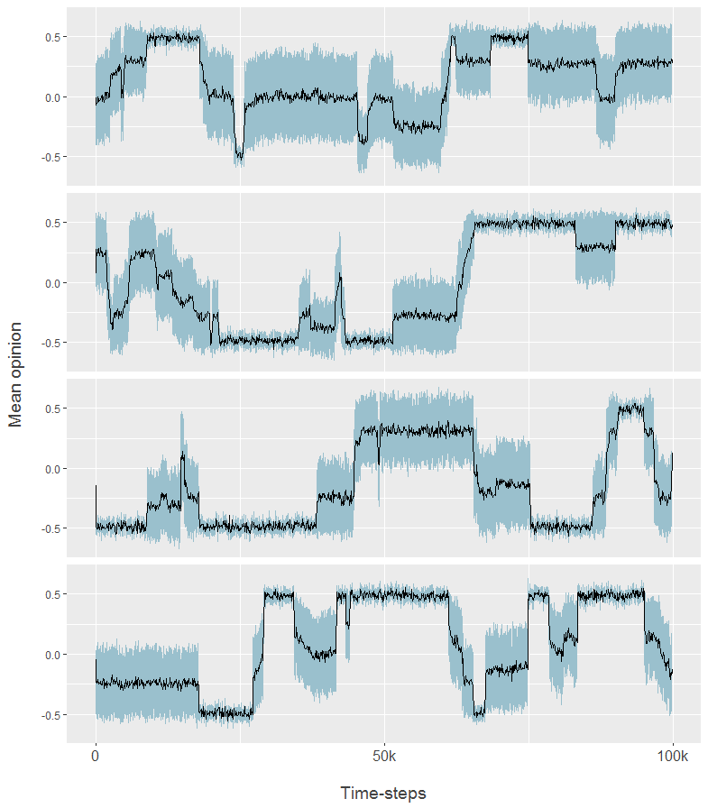
Figure 3 shows different dynamics for each set of initial conditions. In all simulations with all types of networks and parameters, 0.5 and -0.5 act as attractors, obviously as a consequence of the structure of the signals that agents get in each time-step. In RNs and SWNs, the stylized evolution of public opinion (\(\bar{x}_i\)) (leaving aside the small short-term fluctuations in the value of \(\bar{x}_i\)) is either stable at any value between -.5 and .5, or changes monotonically, with -.5 and .5 as unalterable stable states. That is, if \(\bar{x}_i\) changes, we never see a change in the direction of the change, and if this monotonic change reaches either -.5 or .5, then this state will never be altered. We have conducted different simulations keeping \(n\) constant and adding edges to the network, but this pattern is not altered. In RNs and SWNs, the speed at which the system reaches its stability is different in each single simulation and does not seem to depend on \(\mu\). The value of \(\mu\) only seems to affect the small fluctuations in the value of \(\bar{x}_i\), and is greater with higher values of \(\mu\). In sum, we do not observe any transformation of a previously established stable state in these networks.

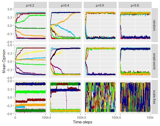
Things are quite different in SFNs. As the parameter \(\mu\) grows, the system shows greater instability, frequently changing from one state to another with no apparent pattern. With lower values of \(\mu\) (\(\mu = 0.2\)) the system is stable or experiences few changes, although we observe rapid soft changes from one state to another after a long period of stability. Mid-low values of \(\mu\) (\(\mu = 0.4\)) more frequently show long periods of stability which are suddenly altered in a rapid soft or rapid-radical process of transition to a new state and, for the first time, we observe a non-monotonic evolution with transitions from higher to lower values and vice versa, in a same dynamic. With higher values \(\mu\) (\(\mu =\) 0.6 and 0.8) the system chaotically and frequently changes from one state to another, generally from one attractor to another (from −0.5 to 0.5 or the other way around), with the frequency of those transitions being higher with higher values of \(\mu\).

Transitions from one stable state to another in scale-free networks are not only changes in \(\bar{x}_i\), but also important changes in the shape of the opinion distribution. As we already saw in Figure 2, the model shows various kinds of transitions, experiencing moments of left-wing (or right-wing) unanimity, moments of a balance between left-wing and right-wing opinions, and moments of unbalance between them.

To mathematically confirm what is visually presented in Figure 3, we calculated the information entropy of each simulation. If we consider this system as a source of information, the different values of \(\bar{x}_i\) can be thought of as the information produced by the system and \(\frac{f_i}{N}\) as the probability of occurrence of each of those states. In this way, the entropy index serves as a measure of the variability of states that a system displays, and in this case, as a measure of the frequency and scope of the fluctuations of the mean opinion. The entropy index (EI) of each simulation can be calculated as follows:

$$EI = -\sum_i \frac{f_i}{N} \ast \log_2 \frac{f_i}{N}$$

(5)

Table 2 shows two different OLS models where we have regressed EI on type of network and \(\mu\). Model 1 shows the positive and statistically significant coefficients of \(\mu\) and scale-free networks. However, Model 2 introduces interaction terms and the coefficient of \(\mu\) is no longer statistically significant. This model proves that \(\mu\) does not have a positive impact on EI by itself, but does have a positive effect on entropy in scale-free networks. The change from small-world to scale-free networks increases the effect of \(\mu\) on the entropy index.

Table 2: OLS regression models: Entropy \(^{\ast}p \leq\)
(1) The parameter \(\mu\) is centered to avoid multicollinearity
(2) Small-world networks as omitted category

	Model 1	Model 2
Constant	2.891\(\ast\) (.149)	2.891\(\ast\) (.112)
\(\mu\) (1)	2.315\(\ast\) (.386)	.059 (.500)
Scale-free (2)	1.688\(\ast\) (.211)	1.688\(\ast\) (.158)
Random (2)	.022 (.211)	.022 (.158)
\(\mu\) \(\ast\) Scale-free		6.176\(\ast\) (.708)
\(\mu\) \(\ast\) Random		.592 (.708)
N	120	120
Adjusted R2	0.496	0.717

The role of homophily

As we have seen in Figure 3, in our model the public opinion dynamics in SFNs show several types of transitions from one state to another. However, it seems clear that the rate of change that we observe with higher values of \(\mu\) is far from representing any natural dynamic. In those, situations, the system too frequently experiences radical transitions from one attractor to the other. Therefore, we must consider that in natural settings where we can assume that agents are embedded in a scale-free network and external signals have a large impact on individual opinions, a counter-balancing mechanism must be at work. Following the lead of bounded confidence models (Deffuant et al. 2000; Krause 2000; Hegselmann & Krause 2002; Weisbuch et al. 2002, 2003), we hypothesized that homophily could be a plausible mechanism to counter-balance the impact of \(\mu\), therefore “softening” the chaotic change in public opinion in such situations.

This mechanism has been widely documented in the literature as one of the sources of homogeneity in peoples’ personal networks (see, for example, McPherson, Smith-Lovin, & Cook 2001). In our case, we state that dyadic similarities can have the effect of softening the impact of high levels of \(\mu\): when external signals align with the opinion of your neighborhood, they jointly attract your opinion, but when they do not align, these opposite attractions may partially cancel each other out, thereby reducing the probabilities of an external, signal induced change in your private opinion.

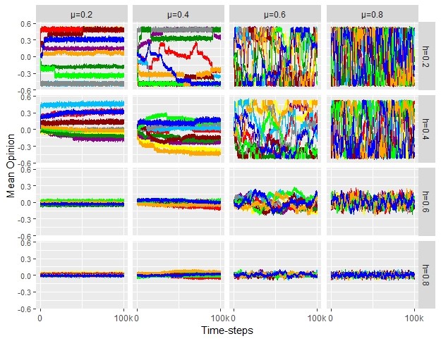
To formalize the role of homophily, we assumed that in each time-step agents only interact with those neighbors whose opinion falls inside a certain interval \(x'_i \pm (1-h)\). The homophily parameter \(h\) is set in \([0,1]\). That is, after determining their provisional opinion (\(x'_i\)), the reference opinion of each agent (\(r_i\)) is calculated only considering those neighbors with \(x_j \in [x'_i - 1 + h; x'_i + 1 - h]\). When agents do not have any neighbors in this interval, they only express their \(x'_i\). Note that even at the lowest value of \(h\), there is some homophily for some agents, since they will only interact with agents in \([x'_i - 1; x'_i + 1]\), so the case when \(h = 0\) is not equivalent to the no-homophily scenario shown in Figure 3.

As expected, low levels of homophily produce the same collective patterns that we saw in Figure 3 (see Figure 4). The higher the homophily, the higher the softening of the radicalness and rate of changes in the mean opinion up to the point where the impact of high values of \(\mu\) is completely neutralized by the high level of homophily. Moderate oscillations between non-attractor but centered points (−0.3 and 0.3, for example) is the rule when intermediate levels \(\mu\) of and \(h\) are combined (\(\mu = 0.6\) and \(h = 0.6\) for example). This is a type of oscillation that we did not see before considering the role of homophily (see Figure 3).

Again, we have calculated the EI (see Equation 5) for each simulation represented in Figure 4 and regressed it on \(\mu\), \(h\), and their interaction term. According to Model 2, there is no independent effect of homophily on entropy, but the effect of \(\mu\) on entropy is higher the lower the values of homophily.

Table 3: OLS regression models: Entropy in scale-free network \(^{\ast}p \leq\) 0.001

	Model 1	Model 2
Constant	3.352\(\ast\) (.174)	1.905\(\ast\) (.284)
\(\mu\)	4.985\(\ast\) (.235)	7.879\(\ast\) (.518)
\(h\)	-3.687\(\ast\) (.235)	-.793 (.518)
\(\mu \ast h\)	NULL	-5.788\(\ast\) (.945)
N	160	160
Adjusted R2	.814	.849

Unraveling the generative process

A black box free explanation of a simulation output is only reached when we unravel its generative process, that is, the micro-level causal chain of events that is responsible for the generation of the (macro-level) output (León-Medina 2017). By tracing this generative process we could answer the most relevant why questions that could be applied to the set of results that we presented in the previous section: why does the stylized evolution of the mean public opinion in RNs and SWNs always remain stable or only change monotonically until the attractor is reached, while this evolution in SFNs is non-monotonic and shows different types of transitions from one state to another? And focusing on SFNs, why do transitions occur? Why are some transitions more radical than others? Why are these transitions in SFNs more frequent and radical (going from one attractor to the other) with higher \(\mu\) values?

The micro-level causal process behind transitions in scale-free networks. We have come to the conclusion that understanding the process behind radical changes (that is, changes from one attractor to the other) in scale-free networks is key to fully understanding the model behavior. This process is characterized by a sequence of steps. We observe soft changes when this sequence is interrupted or reversed. We observe different model behaviors depending on \(\mu\) because this parameter has an influence on the probability that this sequence will occur. We observe changes in scale-free but not in random or small-world networks because they differ in their capacity to trigger this sequence.

Therefore, to understand the inner workings of this simulation, we shall start by analyzing and explaining rapid-radical transitions in scale-free networks. By “radical” transitions we mean shifts from a population of only left-wingers with \(\bar{x}_i = -0.5\) to a population of only right-wingers with \(\bar{x}_i = 0.5\), or vice versa.

One of the keys to understanding abrupt changes in \(\bar{x}_i\) is to be found in the signals that agents get each time-step. It is important to recall here that this signal is randomly chosen for each agent in each time-step from a normal distribution N(0.5,3.5) when \(x_i \geq 0\) or N(−0.5,3.5) when \(x_i < 0\). Considering this standard deviation, an agent can sometimes be subject to signals that are not in line with his \(x\), eventually leading him to change his opinion from \(x_i > 0\) to \(x_i < 0\), or vice versa. That is, it is possible that the mean of the last three signals that the agent gets is not in line with his opinion, therefore pushing him to actualize it (see Equation 1). Once the opinion has changed, the signal that the agent gets is then randomly chosen from the distribution that corresponds with his new opinion, either N(0.5,3.5) or N(−0.5,3.5), thus raising the probability that this agent will stay on that side of the distribution. As we shall see next, this shift in an agent’s opinion is sometimes the triggering event of a causal chain of events that leads the system to a new state.

Generally speaking, a momentary positive value of \(a_i\) is not strong enough to counterbalance the power of social influence and force the agent to a new right- (left-)winged opinion. However, a momentary shift in the sign of \(a_i\) can indeed force a change in opinion in a highly connected agent (an influencer, that is, an agent with a high \(k_i\)), basically because influencers are practically free of the counterbalancing force of social influence (see Equation 4). This shift in the influencer’s opinion can act as the triggering event of a radical social change.

In all the cases of radical changes, the triggering event of the transition is a change in the opinion of the agent with the highest value of \(k\) as a consequence of a momentary shift in the sign of his \(a_i\). Once this change is produced, the influencer does not return to his later side of the opinion distribution, at least in a certain period of time, basically for two reasons. First, because the change is self-reinforced: \(c_i\) and \(a_i\) start working in the direction of keeping the agent on his current side of the distribution (see Equation 1). Second, the agent can resist the influence of his neighbors since this influence is considerably low for agents with higher values of \(k\) (see Equations 2, 3 and 4). If the influencer becomes a right (left-)winger, he will probably remain as a right (left-)winger for a long period of time.

His conversion, however, has important consequences. A set of his neighbors, especially those with lower values of \(k\) (\(k_i = 2\)) and not interconnected, also become right (left-)wingers, one after the other in a first wave of individual transformations. The strong influence of the influencer is higher than his neighbors’ desire for coherence and the signals that they get.

This is the start of a diffusion process. Little by little, and while the transformations that characterize the first wave are still taking place, a second wave of transformations occurs. Agents connected with the influencer but with higher values of \(k\) start flipping their opinion. The key to understanding this second wave of transformations is the agents’ \(r_i\). This reference opinion becomes effective in forcing an opinion change basically through three causal processes (operating in conjunction or separately). First, as external signals fluctuate, some agents momentarily express a more radical opinion, therefore making their neighbors’ \(r_i\) momentarily more extreme. This transitory radicalization is especially effective when it is the influencer that is radicalized. Given the conditions stated in Equation 3, this circumstance considerably maximizes the influencer’s neighbors’ \(r_i\), therefore pushing some of them to change their opinion. Second, a relatively constant \(r_i\) can become effective in forcing a change of opinion if the agent’s opinion is momentarily centered (close to 0) as a consequence of an occasional fluctuation in the value of his \a_i\). And third, as the first wave of transformations advances, the value of an agent’s \(r_i\) can reach the point when it forces an opinion shift simply as a consequence of a rise in the number of newly right- (left-)wing neighbors.

As this second wave of transformations is produced, some of the newly right (left-)wingers’ neighbors with \(k = 2\) also become right (left-)wingers as in the first wave of transformations. As new right- (left-)wingers evolve to values near to the attractor (thanks to the effect of the signals), they win their neighbors over to right (left-)wing positions, thus spreading right (left-)wing opinions all over in a third wave of transformations.

Only when an important proportion of agents have become right (left-)wingers, do left (right-)wing influencers find enough social pressure to become right (left-)wingers. This is an inflection point. When a new influencer’s opinion flips, the same pattern of diffusion triggered by the first influencer is now reproduced among those that still remain on the other side of the opinion distribution: those still left (right-)wingers that are subject to his influence (and that remained left (right-)wingers thanks to that influence), now actualize their opinion one after another.

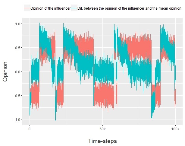
Through these different and partially overlapping waves of individual transformations, right (left-)wing opinions spread through the whole network. The opinion of the highly connected agent that triggered all this process is clearly a powerful leverage point. In SFNs, public opinion always seems to follow the lead of the influencer’s opinion. As we can see in the example of Figure 5, each time the influencer changes his opinion, the difference between his opinion and the mean opinion of the population moves to 0 (sometimes abruptly, sometimes more slowly).

But sometimes this cascade of individual transformations is limited and we only observe a more limited change; a change to a more centered \(\bar{x}_i\), that is, either a slow-soft or a rapid-soft change. An example of these kind of transitions would be a change from a population of only left-wingers and \(\bar{x}_i = -0.5\) to a population with a small fraction of right-wingers and \(\bar{x}_i = -0.3\) or similar. In this case, we observe the same triggering event and the same first wave of individual transformations that we saw in the previous example: an influencer changes his mind as a consequence of the occasional exposure to signals that are not in line with his initial opinion, and this change triggers a first wave of transformations in some of his followers with a low \(k\). However, once this first wave of transformations has moved the mean to −0.3, something stops the process. The first wave of transformations is not strong enough to trigger the second wave. The reason why this is so is to be found in the causal processes that characterize this second wave as we described in the causal narrative of radical transitions: agents change their mind because their \(r_i\) becomes effective in forcing that change, either because its value is maximized when some neighbor (usually the influencer) experiences a transitory radicalization, or because they experience a transitory moderation of their opinion that makes them more vulnerable to the effect of a relatively constant \(r_i\) (or a combination of both situations). If we keep the value of \(\mu\) constant as we do in these examples, these two causal processes just happen or not by chance: they are statistical possibilities that do not necessarily occur. When they do not occur, the cascade of individual transformations is stopped and sometimes even reversed for some agents that return to their original belief, or go back and forth from negative to positive values of \(x\). The system just remains stable at \(\bar{x}_i = -0.3\) for a long period of time until the sequence of steps is restarted or reversed as a consequence of a new change in the influencer’s opinion.

The micro-level causal process behind transitions in different type of networks. Stability or monotonic changes in the stylized evolution of \(\bar{x}_i\) until an attractor is reached are the typical dynamics of our model in RNs and SWNs. Non-monotonic changes characterize SFNs. This different dynamic is the result of one of the main differences in the structure of these types of networks: the degree distribution. There are at least two consequences of this difference.

First, given the power-law distribution of degrees in scale-free networks, most of the existing links of the network are concentrated in only a few agents. As we have already explained, the triggering event of all changes in SFNs is a shift in the opinion of an influencer, and some of the following waves of individual transformations can only happen as the consequence of the influence of these highly connected agents. The highly connected agents in RNs and SWNs are less connected than the highly connected agents in SFNs and are therefore not as influential. This is basically because, given the lower \(k_i\) of these agents, their impact on their neighbors’ \(r_i\) is smaller. The event that triggers a change in the state of the system in SFNs is unable to trigger the same process in RNs and SWNs.

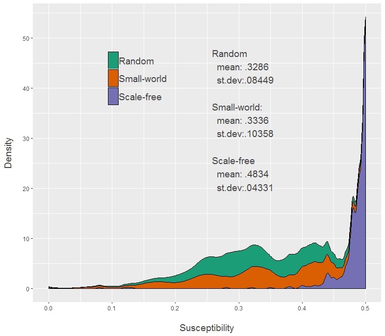
Second, since the degree distribution is different in the three types of networks, the mean and shape of the distribution of \(\theta_i\) is also different. On the one hand, the mean susceptibility to social influence is higher in SFNs than in SWNs and RNs. On the other hand, SFNs show a j-curve distribution of \(\theta_i\), while SWNs and RNs show a negative skew distribution (see Figure 6). Generally speaking, then, the role of social influence is lower in SWNs and RNs, so all the dynamic is more dominated by the other two elements of the decision (\(c_i\) and \(a_i\)), therefore preventing the spreading potential of new ideas through social interaction.

How do we explain then the monotonic tendency of the stylized evolution of \(\bar{x}_i\) towards one of the attractors in SWNs and RNs? There are no initial conditions that could explain why the simulation moves towards one attractor and not the other, not even the initial unbalance between left-wingers and right-wingers that can be produced by chance in the initial configuration of each simulation. Different simulations with the same initial conditions end up in different attractors. Whether the simulation starts a path towards 0.5 or −0.5 depends on who first wins the battle for attracting agents from the other side to their field. Agents with values of \(x\) near to 0 can easily shift from positive to negative values of \(x\) (or the other way around) as a consequence of the fluctuations of \(a_i\). It only depends on chance who wins this initial battle, but once a tendency is started, it cannot be reversed. More agents on one side of the distribution imply a higher power of attraction of that side of the distribution, and there are no influencers whose change in opinion could trigger a reversal of this process of cumulative transformations.

The micro-level causal process behind the impact of \(\mu\). The parameter \(\mu\) is positively correlated with the system instability in SFNs (see Figure 3 and Table 2). The higher the value of \(\mu\), the higher the frequency of abrupt radical changes in the evolution of \(\bar{x}_i\). To describe the mechanism behind this correlation, we should recall here that \(\mu\) fine tunes how much the opinion of the agent is affected by \(a_i\) (the mean of the last three signals that each agent gets). This susceptibility to external signals has three relevant consequences. First, it increases the probability that a momentary accumulation of signals far from an agent’s \(x\) will become strong enough to force him to change his opinion. This is especially important when the agent is an influencer because, as we already saw, this individual transformation could be the triggering event of a social change. The accumulation of signals that could force an opinion change is produced by chance, but the probability that they actually force an opinion change depends on \(\mu\). In fact, the probability that they actually force an opinion change is higher for highly connected agents, since they do not have to deal with the counterbalancing effect of social influence. Therefore, the higher the value of \(\mu\), the higher the frequency of events that trigger a process of change in public opinion.

Second, signals can also lead the agent to a momentary radicalization of his opinion. Again, higher values of \(\mu\) mean that a momentary radicalization of the signals actually radicalizes the individual opinion. And again, this is more likely to happen in influencers. As we already saw, this transitory radicalization plays an important role in system transitions because it transitorily moves the value of \(r_i\) in the influencer’s neighbors away from their initial opinion, therefore pushing some of them to move from left to right, or vice versa (a change that is then self-reinforced as we already explained). In sum, the higher the value of \(\mu\), the higher the probability that the process of individual transformations will spread throughout the network.

And third, since signals are randomly chosen for each agent in each time-step from a normal distribution N(0.5,3.5) when \(x_i \geq 0\) or N(−0.5,3.5) when \(x_i < 0\), a higher \(\mu\) value implies that, even when the signals and therefore the opinion fluctuate, they tend to do so around the attractors. And again, this is more likely to be true for influencers. This is important because an influencer that shifts his opinion from left to right, or vice versa, rapidly tends to fluctuate around the attractor. The farther away from 0, the higher the value of his neighbors’ \(r_i\) and hence the higher the probability that his influence will attract some of them to the left (or right) side of the distribution (especially those neighbors that were on the other side of the distribution but with values of \(x\) close to 0).

Concluding Remarks

With only a few exceptions, the understanding of patterns of public opinion change has generally been dismissed in the literature on opinion dynamics models. To address this theoretical gap in our understanding of opinion dynamics, we have built a multi-agent simulation model that could help us to identify some mechanisms underlying changes in public opinion. The model should be understood as a first attempt to expand our limited knowledge on the collection of mechanisms that could aspire to explaining public opinion fluctuations.

In our model, agents interact in different types of topologies (random, small-world and scale-free networks) and express an opinion that is the result of a coherence mechanism, in which agents try to stick to their previously expressed opinions, an assessment mechanism, in which agents consider available external information on the topic, and a social influence mechanism, in which agents tend to approach their neighbor’s opinions. One of the main features of our model is that, under certain conditions, its behavior is characterized by different types of endogenously (that is, not induced by the researcher) triggered changes in the mean opinion and the shape of the distribution of individual opinions.

Random and small-world networks only show stability or a monotonic tendency towards a definitive stability in one of the attractors of the system. Scale free networks, however, show different types of equilibrium shifts. In fact, the higher the relevance of the external signals that the agents get, the higher the frequency and radicalness of the fluctuations. In fact, transformations of public opinion are basically a diffusion process of the new ideas of the highly connected agents (influencers) in the network. The power law distribution of degrees in scale-free networks and a high value of the parameter \(\mu\) (the subjective relevance of the external signals) are conditions that favor the rapidity, frequency and radicalness of those diffusion processes. In scale-free networks with high values of \(\mu\), fluctuations in public opinion are so frequent and radical that we theorized that a counterbalancing mechanism must be at work in the corresponding natural situations. Following the lead of bounded confidence models, we have shown that homophily can act as this counterbalancing mechanism: high levels of homophily have the effect of “softening” the extent and frequency of public opinion fluctuations, therefore generating softer oscillations. In sum, according to our findings, we should observe more fluctuations in public opinion in natural settings where agents are assumed to be embedded in scale-free networks, and the rate and radicalness of changes should positively depend on how important external information is in individual opinions and negatively depend on how homophilic the social interactions are.

Since this is only our first attempt to tackle the issue of modeling equilibrium changes in public opinion, there are several further directions of analysis that could be pursued in the future. This model could be replicated in other types of networks, and different assumptions of the model could be redefined. For example, agent’s memory could be extended, therefore affecting the coherence mechanism; different structures of the external signs that agents get could be tested; and the relation between agent’s degree and his susceptibility to social influence could be redefined to consider situations where they do not correlate as we assumed. Since we also consider the role of homophily, the model could also be redefined so that we introduce a homophily-guided rewire of links in order to analyze public opinion changes as the network dynamic evolves. Moreover, beyond homophily, the role of alternative counterbalancing mechanisms for the excessive fluctuations we observed under certain conditions could also be explored. In fact, given the general neglect of the study of public opinion fluctuations, there seems to be a whole topic of research ahead of us.

References

ACEMOĞLU, D., Como, G., Fagnani, F. and Ozdaglar, A. (2013). Opinion fluctuations and disagreement in social networks. Mathematics of Operations Research, 38(1), 1-27 [doi:10.1287/moor.1120.0570]

BARABÁSI, A. L. and Albert, R. (1999). Emergence of scaling in random networks. Science, 286(5439), 509-512.

BEM, D. J. (1972). Self-perception theory. Advances in Experimental Social Psychology, 6, 1 62. [doi:10.1016/S0065-2601(08)60024-6]

BURSTEIN, P. (2003). The impact of public opinion on public policy: A review and an agenda. Political Research Quarterly, 56(1), 29-40.

CARLETTI, T., Fanelli, D., Grolli, S. and Guarino, A. (2006). How to make an efficient propaganda. EPL (Europhysics Letters),74(2), 222. [doi:10.1209/epl/i2005-10536-9]

CASTELLANO, C. Fortunato, S. and Loreto, V. (2009). Statistical physics of social dynamics. Reviews of Modern Physics, 81(2), 591-646.

CIALDINI, R.B. (2009). Influence: Science and Practice (Vol. 4). Boston, MA: Pearson Education.

CROKIDAKIS, N. (2012). Effects of mass media on opinion spreading in the Sznajd sociophysics model. Physica A: Statistical Mechanics and Its Applications, 391(4), 1729-1734.

DEFFUANT, G., Neau, D., Amblard, F. and G. Weisbuch. (2000). Mixing beliefs among interacting agents. Advances in Complex Systems 3(01n04), 87-98. [doi:10.1142/S0219525900000078]

DUGGINS, P. (2017). A psychologically-motivated model of opinion change with applications to American politics. Journal of Artificial Societies and Social Simulation, 20(1), 13: https://www.jasss.org/20/1/13.html. [doi:10.18564/jasss.3316]

ERDÖS, P. and Rényi, A. (1959). On random networks. Publicationes Mathematicae, 6, 290 297.

FESTINGER L. (1957) A Theory of Cognitive Dissonance. Stanford, CA: Stanford University Press.

GALAM, S. (1986). Majority rule, hierarchical structures, and democratic totalitarianism: A statistical approach. Journal of Mathematical Psychology, 30(4), 426-434. [doi:10.1016/0022-2496(86)90019-2]

GALAM, S. (1990). Social paradoxes of majority rule voting and renormalization group. Journal of Statistical Physics, 61(3-4), 943-951.

GALAM, S. (1999). Application of statistical physics to politics. Physica A: Statistical Mechanics and its Applications, 274(1), 132-139. [doi:10.1016/S0378-4371(99)00320-9]

GALAM, S. (2000). Real space renormalization group and totalitarian paradox of majority rule voting. Physica A: Statistical Mechanics and its Applications, 285(1), 66-76.

GALAM, S. (2008) Sociophysics: a review of Galam models. International Journal of Modern Physics C, 19(3), 409-440. [doi:10.1142/S0129183108012297]

GARGIULO, F., Lottini, S. and Mazzoni, A. (2008). The saturation threshold of public opinion: are aggressive media campaigns always effective? arXiv preprint arXiv:0807.3937.

GONZÁLEZ-AVELLA, J. C., Cosenza, M. G. and San Miguel, M. (2012). A model for cross-cultural reciprocal interactions through mass media. PLoS ONE, 7(12), e51035. [doi:10.1371/journal.pone.0051035]

HEGSELMANN, R. & Krause, U. (2002). Opinion dynamics and bounded confidence models, analysis, and simulation. Journal of Artificial Societies and Social Simulation, 5(3), 2: https://www.jasss.org/5/3/2.html.

JIANG, L.L., Hua, D.Y., Zhu, J.F., Wang, B.H. and Zhou, T. (2008). Opinion dynamics on directed small-world networks. The European Physical Journal B, 65(2), 251-255. [doi:10.1140/epjb/e2008-00342-3]

KRAUSE, U. (2000). ‘A discrete nonlinear and non-autonomous model of consensus formation.’ In Elyadi, S., Ladas, G., Popenda, J. and Rakowski, J. (Eds.) Communications in Difference Equations. Amsterdam: Gordon and Breach Pubm, pp. 227–236.

KURAN, T. (1987a). Chameleon voters and public choice. Public Choice, 53(1), 53-78. [doi:10.1007/BF00115654]

KURAN, T. (1987b). Preference falsification, policy continuity and collective conservatism. The Economic Journal, 97(287), 642-665.

KURAN, T. (1989). Sparks and prairie fires: A theory of unanticipated political revolution. Public Choice, 61(1), 41-74. [doi:10.1007/BF00116762]

KURAN, T. (1990). Private and public preferences. Economics and Philosophy, 6, 1-26.

KURAN, T. (1991a). Cognitive limitations and preference evolution. Journal of Institutional and Theoretical Economics, 146, 241-273.

KURAN, T. (1991b). Now out of never: The element of surprise in the East European revolution of 1989. World Politics, 44(01), 7 48.

KURAN, T. (1995). Private Truths, Public Lies: The Social Consequences of Preference Falsification. Cambridge: Harvard University Press.

LAGUNA, M. F., Abramson, G. and Iglesias, J. R. (2013). Compelled to do the right thing. The European Physical Journal B, 86(5), 202.

LATANÉ, B. (1981). The psychology of social impact. American Psychologist, 36(4), 343-356. [doi:10.1037/0003-066X.36.4.343]

LEÓN-MEDINA, F. J. (2017). Analytical sociology and agent-based modeling: is generative sufficiency sufficient? Sociological Theory, 35(3), 157-178.

LORENZ, J. (2007). Continuous opinion dynamics under bounded confidence: A survey. International Journal of Modern Physics C, 18: 1819. [doi:10.1142/S0129183107011789]

MANZA, J., Cook, F. L. and Page, B. I. (2002). ‘The impact of public opinion on public policy. The state of the debate.’ In Manza, J., Cook, F. L., and Page, B. I. (Eds.). Navigating Public Opinion: Polls, Policy, and the Future of American Democracy. New York: Oxford University Press, pp. 17-32.

MCPHERSON, M., Smith-Lovin, L. & Cook, J.M. (2001). Birds of a feather: Homophily in social networks. Annual Review of Sociology, 27(1), 415-444. [doi:10.1146/annurev.soc.27.1.415]

MOUSSAÏD, M., Kämmer, J.E., Analytis, P.P. and Neth, H. (2013). Social influence and the collective dynamics of opinion formation. PLoS OONE, 8(11), e78433.

QUATTROCIOCCHI, W., Caldarelli, G. and Scala, A. (2014). Opinion dynamics on interacting networks: media competition and social influence. Scientific Reports, 4, 4938. [doi:10.1038/srep04938]

SÎRBU, A., Loreto, V., Servedio, V. D. and Tria, F. (2017). ‘Opinion dynamics: models, extensions and external effects.’ In Loreto, V., Haklay, M., Hotho, A., Servedio, V. D., Stumme, G., Theunis, J., & Tria, F. (Eds.). Participatory Sensing, Opinions and Collective Awareness. Berlin Heidelberg: Springer, pp. 363-401.

SOBKOWICZ, P. (2009). Modelling opinion formation with physics tools: Call for closer link with reality. Journal of Artificial Societies and Social Simulation, 12(1), 11: https://www.jasss.org/12/1/11.html.

VAN MARTINS, T., Pineda, M. and Toral, R. (2010). Mass media and repulsive interactions in continuous-opinion dynamics. EPL (Europhysics Letters), 91(4), 48003.

WANG, S.-W., Huang, C.-Y. and Sun, C.-T. (2013). Modeling self-perception agents in an opinion dynamics propagation society. Simulation, 90(3), 238-248. [doi:10.1177/0037549713515029]

WATTS, D. J. and Strogatz, S. H. (1998). Collective dynamics of ‘small-world’ networks. Nature, 393(6684), 440-442.

WEISBUCH, G., Deffuant, G., Amblard, F. and Nadal, J.P. (2002). Meet, discuss and segregate! Complexity, 7(3),55–63. [doi:10.1002/cplx.10031]

WEISBUCH, G., Deffuant, G., Amblard, F. and Nadal, J.P. (2003). ‘Interacting agents and continuous opinions dynamics.’ In Cowan, R. and Jonard, N. (Eds.) Heterogenous Agents, Interactions and Economic Performance Berlin, Heidelberg: Springer, pp. 225-242.

WLEZIEN, C. and Soroka, S. N. (2007). ‘The relationship between public opinion and policy.’ In Dalton, R. J., and Klingemann, H. D. (Eds.). The Oxford Handbook of Political Behavior. Oxford: Oxford University Press, pp. 799-817. [doi:10.1093/oxfordhb/9780199270125.003.0043]

ZHANG, W., He, M.S. and Jin, R. (2013). Opinion dynamics in complex networks. Lithuanian Journal of Physics, 53(4), 185-194.