ABOOMS: Overcoming the Hurdles of Continuous-Time Public Goods Games with a Simulation-Based Approach

Introduction

In Agent-Based Modelling and Simulation (ABMS), a system is modelled as a collection of agents, which are autonomous decision-making units with diverse characteristics (Macal & North 2010). The individual agents interact with each other and their environment at the micro level to produce complex collective behaviour patterns at the macro level, often referred to as system level emergence. ABMS supports the representation, experimentation and analysis of complex social phenomena to gain an understanding of the dynamics behind them (Elsenbroich & Gilbert 2014). In Economics, Public Goods Games (PGGs) are one of the most popular types of experiment that has previously been modelled by applying ABMS. ‘Public goods’ are goods that people can consume without reducing their availability for others, such as broadcast television, radio signals and street lights. Pure public goods are non-excludable (a person cannot be prevented from enjoying their benefits) and non-rival (benefits are the same for everyone). In experimental economics, human cooperation in the context of public goods is studied by using a strategic situation as described by PGGs. Laboratory experiments of PGGs have found that there is variability in behaviour: some individuals prefer to cooperate while others prefer to free ride (Fehr & Gächter 2002; Fischbacher et al. 2001). There have been many variations of PGGs to study cooperation behaviour in different settings.

Most PGG experiments are conducted in discrete time. People make decisions synchronously in one round (and therefore don't know anything about others' decision in that round), receive information such as average contribution, then move on to the next round and repeat the game. However, most real-life PGG situations have a real-time aspect, which can alter the interaction nature in fundamental ways (Simon 1989). One example of continuous-time PGG is a website where everyone can contribute contents such as Wikipedia or Reddit. A user of these websites can contribute by interacting (posting, voting, commenting, etc.) in continuous time, and everyone can consume the content (e.g. view a verified page on a topic on Wikipedia or the top-voted list of contents on Reddit). There are game theoretic analyses of continuous-time games (Bergin 1993; Laraki 2005; Sannikov 2007; Neyman 2017), and some laboratory experiments (Dorsey 1992; Friedman 2012; Oprea 2014), but overall the literature on continuous-time PGGs is very sparse when compared to discrete-time PGGs. Regarding the laboratory experiments, researchers have used some workarounds to create continuous-time PGGs. Dorsey (1992), for example, allows participants to change their contributions in continuous time during each round (consisting of a specific period of time), but only the final decisions of the periods are calculated for payment. Oprea (2014) also considers continuous-time PGG lab experiments but with continuous flow-payoff setting. The stumbling block is that a dynamic environment, created by the real-time aspect, allows complex interactions which are difficult to model. To our knowledge, there is no agent-based simulation that studies continuous-time PGG. Additionally, to model such an environment requires a framework that supports the development of models that allow capturing these complex dynamics in continuous time.

Many studies (e.g. Lucas et al. 2014; Amin et al. 2018) have utilised the observed behaviour and data collected from PGG laboratory experiment to build simulation models and performs further experiments without the restrictions of the laboratory environment, which are: limited time, limited budget, problems with recruiting participants, etc. However, there are many concerns related to the little use of Software Engineering (SE) methods in ABMS and the need for standards. Siebers & Davidsson (2015) introduce a JASSS special section of the current state-of-the-art in using SE methods in ABMS. Rossiter (2015) addresses the structural design of simulations by outlining three best-practice properties of SE and mapping the architecture of these simulation toolkits. Rossiter also stresses the little focus of SE and cultural issues in its adoption where people are “introducing everything by analogy and simulation-specific terminology, ’hiding’ the generic SE origins and thus obscuring the interdisciplinary links.” Collins et al. (2015) discuss the use and need for standards for ABMS. Following this line of thought, we believe that ABMS has not been used to its full potential by social scientists, due to the lack of guidance on how to develop these models, and that a more formal approach using ideas from SE could help to improve the situation. In order to fulfil this need, Vu (2017) developed a framework called the Agent-Based Object-Oriented Modelling and Simulation development framework (or ABOOMS framework for short).

In this paper, we introduce the ABOOMS framework (Section 2) and describe an application of the ABOOMS framework to rigorously develop an agent-based simulation of continuous-time PGGs (Section 3). We then briefly analyse the simulation results and discuss the development of the best practices for building agent-based social simulation models (Section 4) before we conclude and present a future outlook in (Section 5).

Introduction to the ABOOMS Framework for PGGs

The important concepts from software engineering

Since a simulation is software, its development involves many SE techniques. When implementing a simulation model, in general, there are two approaches: programming it from scratch or using a simulation software package. Both approaches usually use an Object-Oriented Programming (OOP) language to define the model and its execution. OOP is a mainstream implementation method in which software is organized as a collection of objects, each of which is an instance of a class (which is a template for creating objects).

The process that is used for developing object-oriented software is called Object-Oriented Analysis and Design (OOAD). The fundamental idea of OOAD is to break a complex system into its various objects (Booch 2007). One of the most important design principles in SE is the separation of concerns, which is the idea of separating computer software into sections such that each section addresses a separate concern and overlaps in functionality are reduced to a minimum. With this design principle, OOAD supports reusability and extensibility (Graham et al. 2000). Reusability is the use of existing assets in software development such as code, templates, components, frameworks, patterns, etc. Extensibility is the ability to extend the system with minimal effort and risk to the existing system. Because of these benefits, OOAD is used as a base for the lifecycle of the ABOOMS framework.

There are many OOAD processes in SE, which all use the same graphical notation for communication and documentation - the Unified Modelling Language (UML). UML was developed by Grady Booch, James Rumbaugh, and Ivar Jacobson in the 1990s and is widely used due to its flexibility, extensibility, and independence of the OOAD processes (Deitel & Deitel 2007). It provides a feature-rich graphical representation scheme for the modeller to develop and document their object-oriented systems. In the ABOOMS framework, it is recommended that UML diagrams are utilized during the development lifecycle to support the process as well as producing the documentation for the model.

The ABOOMS development framework

This section provides a short introduction to the ABOOMS framework. Further details on the development with the ABOOMS framework are provided in Vu (2017). Here we first look at the macro-level development process, which guides the overall development life-cycle of the study. Then, the micro-level development processes, which incorporate the analysis and design techniques and principles (OOAD) for simulation development are presented. Please note that in this paper we use the ABOOMS framework in the context of PGG; however, it can also be generalized to other economic experiments.

The macro-level development process

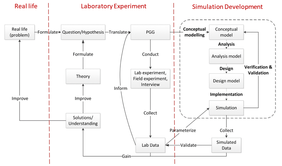
The life cycle of the ABOOMS framework is shown in Figure 1. It is split into three main sections: (1) the real life, (2) the laboratory experiment, and (3) the simulation development. Each section contains components (rectangle) and processes (arrows). In Figure 1, the area of a dashed rounded rectangle marks where OOAD is applied and contains five processes (arrows with bold labels). These processes are the micro processes and will be described in detail after the macro process.

A question/hypothesis (in laboratory experiment session) can be formulated from a real-life problem and/or a theory. Then a simplified version of the situation, a PGG, is created. From the PGG, a lab experiment is designed and conducted to collect human behaviour data. To start the simulation development, a conceptual model is constructed from the PGG. Then a simulation is developed from the conceptual model using an OOAD process. In OOAD, the analysis process produces an analysis model that contains the interactions between the system and its environment. The next step is to design the system to solve the issue identified in the analysis model, resulting in a design model. The final step of OOAD is to implement the simulation from the design model. The data collected from the lab experiment can be used to parameterize the simulation. Since the simulation is based on the laboratory experiment, the simulated data can be used to support the validation of the laboratory data. Finally, using the simulation and laboratory experiment, modellers and domain experts gain better understanding, improve their capacity to answer the formulated question or confirm the hypothesis, thus improving theory or solving real-life problems.

The micro-level development processes

In this section, the five development processes (the arrows with bold labels in the dashed rounded rectangle of Figure 1) are described in more detail. In each process, there are multiple steps which guide the development of the simulation.

• Process I - Conceptual Modelling
  • Step I.1: Understand the problem situation.
  • Step I.2: Determine objectives of the simulation study.
  • Step I.3: Collect and analyse data and related theories.
  • Step I.4: Identify the settings of the PGG (such as scheduling, players’ possible actions, or other game rules).
  • Step I.5: Design the conceptual model: experimental factors, responses, model content, assumptions and simplifications.

• Process II - Analysis
  • Step II.1: Identify actors including agents, artefacts, and external actors:
    • Agents (internal actors): autonomous, proactive entities that encapsulate control and in charge of goals/tasks that altogether determine the whole system behaviour. For example, in PGG, players are agents.
    • Artefacts (internal actors): passive, reactive entities that are in charge of required services and functions that make agents work together and shape the agent environment. For example, in PGG, an artefact can be a "game master" to inform players of the current stage of the game.
    • External entities (external actors): entities that interact with the simulation system such as human and other systems. It can be useful for interactive simulations where modellers have to define interactions between the system and users.
  • Step II.2: Identify use cases. A use case can be a behaviour to be exhibited by agents, or an interaction between agents and external actors, or between agents.
  • Step II.3: Draw Use Case Diagram.

• Process III - Design
  • Step III.1: Define structure (internal data, operation) by using Class Diagrams.
  • Step III.2: Define behaviour by using behavioural diagrams, such as Statechart, Sequence Diagram, Activity Diagram.

• Process IV - Implementation
  • Step IV.1: Choose a programming language and/or a software: The simulation can be programmed from scratch or with a specialist simulation toolkit (such as NetLogo, AnyLogic, Repast Simphony).
  • Step IV.2: Programming, testing and debugging.

• Process V - Verification and Validation
  • Step V.1: Verify whether the simulation correctly implemented the conceptual model.
  • Step V.2: Validate and tune agent behaviour based on the information from the lab or

After introducing the ABOOMS framework, the principles behind it, as well as the details required for the development, the framework will be applied to a case study to demonstrate its capabilities.

Case Study of Continuous-Time PGG

In this section, the ABOOMS framework is employed to develop a simulation of a PGG experiment played in continuous time where participants can change their contribution at any time. In Section Section 3.2-3.4 we briefly describe the laboratory experiment of a continuous-time PGG that our case study is based on. Then in Section 3.5-3.26, the simulation development is explained in detail by following the micro processes of the ABOOMS framework.

From laboratory experiment to simulation study

Our case study is based on an experimental work on continuous-time PGGs by Oprea et al. (2014). The goal of their work is to study cooperative behaviour in a continuous time setting, which is a complex aspect of most real-life public goods. Oprea et al's laboratory experiment varies two experimental treatments:

• Timing protocol (discrete vs. continuous time) For a game in discrete time, the participants make a decision every minute for 10 rounds (10 minutes in total), and payoff for each round is calculated every minute. In continuous time, the participants make contributions in 10-minute intervals, can change their contribution at any time during this interval, and receive a flow payoff (payoff is divided into smaller portions for a shorter time period). For example, a payoff function \(f\) is used in discrete time to calculate the payoff every minute. In a continuous time game where the payoff is calculated every 100 ms, the payoff function for every 100 ms will be \(f' = \frac{f}{600}\) because \(1 \text{minute} = 600 \times 100 \text{ms}\).
• Communication protocol (no-communication vs. free-form communication) The participants cannot communicate in any way in a no-communication protocol. On the other hand, in free-form communication, participants can communicate with other group members by typing any text in a chat window.

Oprea et al. (2014) report a slightly improved contribution for continuous time experiments compared to discrete time experiments but could not reach mutual cooperation, and free-form communication substantially raised the contribution compared to no-communication. Since free-form communication contains substantial amounts of noise, it is very hard to identify the elements that drive contribution in this setting. Therefore, the case study conducted in this paper focuses on the no-communication setting. The experiment of Opera et al. shows that in no-communication experiments, the participants start to use pulses in contribution as an effort to communicate. A pulse is a situation when one increases his contribution to a very high value (often the maximum value) then drops down to the previous level immediately. These pulses may be used as signals of cooperation, but we cannot be certain that all the pulses are seen or how they are interpreted by other parties. The participants could miss the pulse, not understand the signal, or see it but still wait for responses from others. Without communication, the intention of the pulses is ambiguous.

In our case study, the first question to answer is how much do these pulses influence the contribution? When performing a pulse, people have different rates: some wait for a while before dropping down; others drop down immediately. In addition, we hypothesize that the slight increase of contributions in continuous time is not only caused by the ability to create a pulse as an attempt of communication, but also by the ability to evaluate and contribute asynchronously. With the asynchronous decision making, people can evaluate at different frequencies. Some evaluate and change their contribution frequently; while for others, there is a longer break between two evaluations. Therefore, the second hypothesis is that the evaluation rate (fast and slow) can also affect the group contribution. In summary, the case study explores how the two behaviours (pulse and asynchronous evaluation) influence contributions in continuous time. Also to the best of our knowledge, this is the first time that an agent-based simulation for a continuous-time PGG has been developed.

Developing the simulation model

After we have discussed the real-world problem and the laboratory experiment above, we now focus on the simulation model development, i.e. the micro-level development processes presented in Figure 1 and described in Section 2.7-2.8.

Process I - Conceptual modelling

Step I.1: Understand the problem situation

This step is to make sure that the conceptual model better captures the strategic interaction or situation. Because the case study is based on a lab experiment, this step will discuss the settings of the laboratory experiment. In the experiment of Oprea et al. (2014), the participants were arranged into groups of four. They played the PGG in their group using a computer. Each received an endowment of 25 tokens. Each token invested into the public goods became 1.2 points and was shared between group members. The payoff is calculated by Equation 1.

$$\pi_i = 25 - g_i + 0.3 \sum_{j=1}^4 g_j$$

(1)

where a pay-off (\(\pi\)) for a participant \(i\) is defined by their contribution (\(g_i\)) and the sum of contributions of all players in the group.

Participants can change their contribution at any time by using a slider at the bottom of the graph. Everyone can see contributions as well as payoffs of others in their group. For each game, participants play for 10 minutes and the payoffs are calculated by a utility flow function over time.

Step I.2: Determine the objectives of the simulation study

The objective of the simulation study is to investigate how the two following behaviours can influence the contribution in continuous-time PGG: pulse behaviour and evaluation rate.

Step I.3: Collect and analyse data and related theories

In this step, we explore the related experiments and have a closer look at the data available from Opera et al.’s experiment. To the best of our knowledge, there are two laboratory experiments of continuous-time PGG: Dorsey (1992) and Oprea et al. (2014). In the experiments of Dorsey (1992), participants can change their contribution throughout the game but only the final decisions of the periods are calculated for payment. Oprea et al. (2014) performed continuous-time experiments but with continuous flow payoff setting which is strategically different from Dorsey’s work.

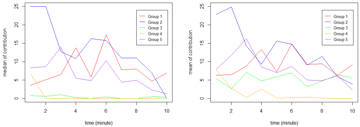
With the data from the experiments of Oprea et al. (2014), we can analyse the participants’ behaviour in the no-communication continuous-time setting. There are five groups of four playing in that setting over ten minutes. Figure 2 shows the median and mean of contributions for every minute. In Figure 2a, generally, the median of contribution decreases over time: Contribution of Groups 3 and 4 drops to near 0 in the second round; Group 2 starts at full contribution then decreases over time; Group 1 and 5 begin with low contribution then oscillate before diminishing. Although the contribution of the whole population decreases, there are different dynamics of behaviour in the five groups. Thus we decided to categorize the behaviour of agents into different types as an attempt to understand and explain the group dynamics. These categories are based on our observation of the experiments conducted by Opera et al and presented in Oprea et al (2014). They are not derived from any other literature. There are five types of behaviour:

1. (Wary) Cooperator: People that contribute maximum value for a long time (up to 1-2 minutes), then drop to zero contribution (probably when dissatisfied), but later increase their contribution to maximum again. The total time they contribute is around a third of the total game time. From this point onward, we will use the term “Cooperator” instead of “Wary Cooperator” for simplification. Keep in mind that this “Cooperator” term is not the same as the “Unconditional Cooperator” term used in the discrete-time PGG literature. Unconditional Cooperators always contribute; on the other hand, our Cooperator contributes for long periods and does not at all contribute for shorter periods.
2. Generous Conditional Cooperator (GCC): People who match their contribution to the average of other members in the group, and sometimes increase contribution for a short period of time (i.e. a pulse).
3. Conditional Cooperator (CC): People who match their contribution to the average of other members in the group.
4. Defector: People who contribute 0 most of the time (with noises).
5. Noisy Player: People who change contributions frequently and to a wide range of values from 0 to 25.

Table 1: Individuals in no-communication continuous-time experiments

ID	Group	Type	Rate of change	No of pulses
102	1	noisy player	2.42
103	1	GCC	1.85	3
107	1	GCC	1.30	8
108	1	GCC	1.86	6
111	2	CC	0.73
114	2	CC	0.42
115	2	CC	0.91
116	2	cooperator	1.42
202	3	defector	1.04
203	3	defector	0.51
204	3	GCC	1.36	12
205	3	cooperator	0.99
216	4	defector	0.43
218	4	defector	0.24
2110	4	GCC	0.27	3
2112	4	CC	0.48
221	5	GCC	3.13	25
227	5	noisy player	5.31
229	5	cooperator	1.30
2211	5	CC	0.58

Table 2: Number of each type in no-communication continuous-time experiments

Type	Count
cooperator	2
GCC	7
CC	5
defector	4
noisy player	2
Total	20

Table 1 shows the classification of behavioural type of each participant. The table also shows the rate of change, that is calculated by the function \(\sum_{t=1}^{600} g_t - g_{t-1}\) where \(g_t\) is the contribution at \(t\) second (all agent starts with an initial contribution at time \(t=0\), randomly based on their type). For GCCs, the number of pulses (in 10 minutes) is also counted. During a pulse, the contribution increases to a high value, which is greater than 20, and stays at that level for as short as 1 second or up to 15 seconds. Table 2 is the count of each type and is used to estimate the percentages of each types and use them to parameterize the simulation. For our simulation, the noisy player is excluded to eliminate unnecessary noise. The remains four types are estimated as follows:

• 10% of Cooperators.
• 40% of GCCs.
• 30% of CCs.
• 20% of Defectors.

Step I.4: Identify the settings of the PGG

The settings of the PGG are:

• Group structure: groups of four people.
• One-shot or repeated games: repeated games.
• Players’ action: evaluate, contribute, pulse.
• Scheduling: continuous-time and asynchronous decision making.
• Game loop: There is no control loop. The players change contribution any time during the game and receive flow payoff.
• Payoff function: Equation 1.
• Information: players know the contribution of each player in the group.

Step I.5: Design the conceptual model

The framework required the following details for the conceptual model:

• Inputs (Experimental factors):
  • Different ratio of behavioural types.
  • Rate of evaluation.
  • Rate of staying generous, i.e. pulse (higher rate means more time staying at high contribution).
• Outputs (Responses):
  • Average contribution over time.
  • Contribution of each agent over time.
• Model Content:
  • Scope in Table 3
  • Level of details in Table 4
• Assumption:
  • People do not change strategy in all rounds of the game.
  • There are no noisy players.
  • Ratio for the base experiment: 10% of cooperators, 40% of GCCs and 30% of CCs, 20% of defectors.
  • GCCs perform pulse on average 7 times during 10 minutes, or 0.7 times per minute. (based on the median of the number of pulses in Table 1).
• Simplification:
  • People cannot communicate in any way.
  • People have complete and common knowledge of the game structure and payoffs.
  • Agents take 500 ms to evaluate and 500 ms to change their contribution.

Table 3: Model scope

Component	Include/Exclude	Justification
Person Communication	Include Exlude	Required for decision making No-communication setting which means the agent cannot send messages to communicate intention or negotiate.

Table 4: Model level of detail

Component	Detail	Include/Exclude	Comment
Person	Contribution Others’ contribution Strategy	Include Include Include	The result of decision making. Information required as inputs of decision making. Required for decision making.

After understanding the problem and having a conceptual model, the next process, Analysis, will organize the requirements around actors base on the conceptual model and identify the interactions of these actors with the environment.

Process II - Analysis

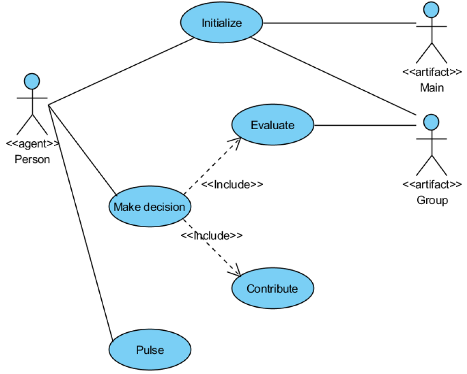
Step II.1: Identify actors

There is one type of agent, a Person agent, that represents a participant in the game. Each Person agent is assigned to a Group, which is an artifact. The Group artifact manages the contribution of the group, calculates the contribution and the payoff for Person agents. There is also a Main artifact that initializes the agent population and collects statistics. In summary, there are three internal actor types: Person agents, Group artifacts, and a Main artifact.

Step II.2: Identify use cases

From the description of actors, the next step is to identify use cases that can be performed by the actors. For the game in this case study, there are five use cases:

1. Initialize: Main initializes the properties of Person agents, and randomly shuffles them into groups of four.
2. Make decision: Person agents evaluate [Evaluate use case], then contribute [Contribute use case].
3. Evaluate: Person agents update their belief (learn from experience).
4. Contribute: Person agents make a contribution based on their type.
5. Pulse: Person agents increase contribution to a high value then drop down.

Step II.3: Draw use case diagram

Figure 3 shows the use case diagram. There are «include» relationships between “Make a decision” (the including use case) and “Evaluate” and “Contribute” (the included use cases). After the Analysis process, we have a use case diagram which captures an understanding of actors and their use cases. Based on the use case diagram along with the use case description, modellers can start the Design process to define the software architecture.

Process III - Design

Step III.1: Structural design

From the actors, there are three classes representing Person agent, Main artefact, and Group artefact. Main class links to the Person and Group classes by association relationship, allowing the Main class to initialize and manage those two classes. There is an aggregation relationship between Person and Group classes: a Group contains four Persons, and a Person can only belong to one Group.

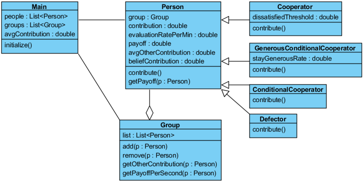
Because there are major differences in behaviour between types of Person agents, such as pulse behaviour of GCCs compared to dissatisfied behaviour of cooperators, inheritance is employed in the structural design to capture the semantics of the type hierarchy. Person is the superclass, and each of four types is a subclass (i.e. aggregation relationship between Person and Group class). So there are seven classes in total, shown in the class diagram Figure 4. The four subclasses inherit attributes and behaviours of Person superclass, but still have their own attributes and behaviours. For example, the group variable of Person class is inherited by subclasses, but contribute() operation is overridden by each subclass to implement their own behaviour.

Step III.2: Behavioural design

At the beginning of a simulation run, Main sets up the ratio of different behavioural types of Person agents, initializes their belief and contribution, and randomly adds Person agents into different groups of four. During the simulation run, Main collects statistics on contributions every second. Each simulation runs for 10 minutes, so there are 600 points of data per participant.

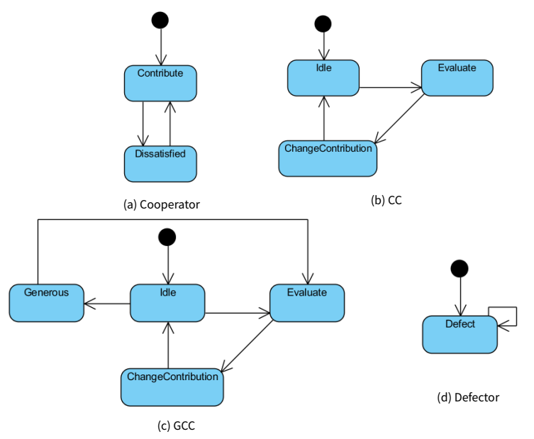
For the four types of agents (Cooperator, GCC, CC, Defector), each has a statechart to represent different contribution behaviours (Figure 5). The Person agent has two variables that are frequently used in the statecharts: evaluateRatePerMin is the rate at which agents evaluate and make decisions; and avgOtherContribution is the average contribution of other group members. The detailed description of each statechart is as follows:

• The statechart of Cooperator agents, shown in Figure 5a, has two states: Contribute and Dissatisfied. When in Contribute state, cooperators contribute 25. The transition from Contribute to Dissatisfied is triggered by the rate evaluateRatePerMin, with a guard condition that avgOtherContribution is less than dissatisfiedThreshold. The transition from Dissatisfied to Contribute is triggered by a rate of 1 time per minute. More specifically, the durations between transition triggers are distributed exponentially and have an average of 1 minute. So on average there is 1 transition per minute.
• Figure 5b is the statechart of CCs with three states: Idle, Evaluate, ChangeContribution. The transition from Idle to Evaluate is rate triggered with the rate evaluateRateP erM in. When entering Evaluate, an agent requests the avgOtherContribution from the Group artifact, and then updates its belief Contribution. The transitions from Evaluate to ChangeContribution and from ChangeContribution to Idle have a timeout of 500 ms. Simplification has been made here: agents take 500 ms to evaluate and 500 ms to change their contribution.
• The statechart of GCCs, illustrated in Figure 5c, is an extension from the statechart of CCs by adding a Generous state. The transition from Idle to Generous is rate triggered (0.7 per minute as explained in the assumption of conceptual modelling). The transition from Generous to Evaluate is triggered with a rate stayGenerousRate.
• Figure 5d is the statechart of Defectors with only one state. There is a self-transition with the rate of evaluationRatePerMin.

For the Evaluate use case, due to the small number of participants in the lab experiment of Oprea et al. (2014), we decided to not derive belief equation from Oprea et al.’s data, but made an assumption. Agents update their belief beliefContribution based on their current belief and belief of other people in the group: beliefContribution = 0.5 x avgOtherContribution + 0.5 x beliefContribution.

For the Contribute use case, the agents use the following equations for making a contribution decision:

• Cooperator: contribution = 25
• Defector: contribution = 0
• GCC and CC: contribution = beliefContribution

3.2.4 Process IV - Implementation

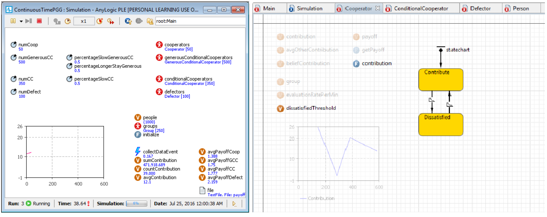
After the design, a simulation can be implemented to explore the question identified at the beginning of the case study. The simulation was implemented with AnyLogic 8 PLE (The AnyLogic Company 2018) and is available online at CoMSES Computational Model Library (Vu 2018). Figure 6a shows the Main screen during simulation experiments. For inheritance, AnyLogic IDE shows the superclass elements as transparent in the IDE view of the subclass. Figure 6b is the IDE view of the Cooperator agent. The transparent elements (7 variables, 1 function, and 1 time plot) are inherited from Person superclass. Other elements (dissatisfiedThreshold variable, contribution function, and a statechart) are its own attributes and behaviours.

The seven parameters (related to the inputs identified in the conceptual modelling process) shown on the left side of the Main screenshot (Figure 6a) can be varied for simulation experiments. For the first experimental factor (ratio of agent strategies), four parameters are required for percentages of four agent strategies: numCoop, numGCC, numCC, numDefect. The sum of these four parameters is 1000 agents. The other two experimental factors, rate of staying generous and rate of evaluation, are ranged from 0 to 1. For the experiments to be manageable, the evaluation rate is set to either slow rate (5 per minute) or fast rate (30 per minute). For example, if the evaluation rate of an agent is slow, it means that agent, on average, evaluates 5 times per minute, i.e. evaluates every 12 seconds. For the fast evaluation rate of 30 per minute, agents, on average, evaluate every 2 seconds. The rate of staying generous is set to one of the same two values as evaluation rate but with different names: longer stay generous (5 per minute) and shorter stay generous (30 per minute). Three parameters are introduced: percentageSlowGCC, percentageLongerStayGenerous, and percentageSlowCC to represent the percentages of different rates in the population of GCCs and CCs.

Process V - Verification and Validation

During the development of the simulation model, we have conducted many verification and validation exercises, in order to produce an accurate and credible model. For the verification we have ensured that the model is programmed correctly, the algorithms have been implemented properly, and the model does not contain errors, oversights, or bugs (North and Macal 2007). We have conducted validation at all stages of development, from conceptual modelling to implementation. Mainly we have used the expert opinion informed by Oprea et al. (2014). For the tuning of the agents, we have used the information provided in their paper (Oprea et al. 2014).

Experimentation and results

GCC agent type

As a thought experiment, we can draw a conclusion that the ratio of different agent types affects the initial contribution and the contribution dynamics over time. The initial contribution of each type is specific: Cooperators start with 25 MUs (Money Units), Defectors start with 0 MU, GCCs and CCs start with 12.5 MU on average (MUs of GCCs and CCs are uniformly distributed between 0 and 25). Thus, with a large population of agents, the average initial contribution of a simulation is the weighted average of initial contributions of all different types. The contribution dynamics are driven by the GCCs and CCs because they are the only two types that change their behaviour. Another factor is the percentages of Cooperators and Defectors since GCCs and CCs response to the behaviour of others: in general, more Cooperators drive the contribution up while more Defectors will lower the contribution level. Lastly, because the GCCs are making pulses, these periods of increasing contribution can pull the contribution up temporarily or permanently. In short, the ratio of different agent types is crucial to simulation results.

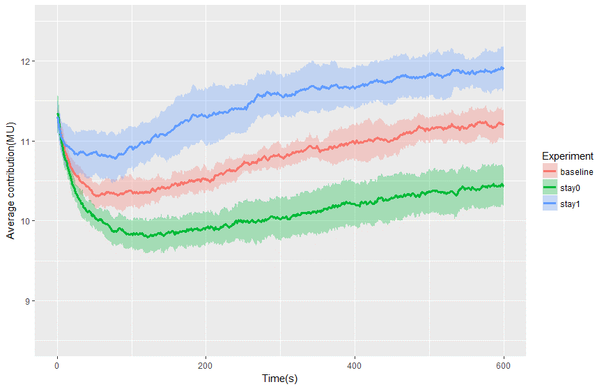
In the limited scope of this paper, we decided to design experiments with a focus on the effect of the new GCC type. The design of experiments is described in Table 5. Firstly, as a baseline experiment, we set up the ratio of agent types to be similar to the ratio from the laboratory experiment of Opera et al. (Table 2): 10% Cooperators, 20% Defectors, 40% GCCs, and 30% CCs. With 1000 agents in total, we arrived at the parameters of the “baseline” experiments in Table 5. In the baseline experiment, the percentages of people with slow evaluation rate and stay generous longer are set to 50%. Then we varied the three parameters of GCCs to the minimum and maximum value: (1) numbers of GCC and CC - numGCC, (2) the percentage of slow GCC - percentageSlowGCC, and (3) the percentage of longer-stay-generous GCCs - percentageLongerStayGenerous. In Table 5, the parameters different from the baseline experiment are in bold. For each experiment, there were 10 replications and the agent contribution decisions were collected every second. Then the whole-population average contributions over time and standard deviation of 10 replications were calculated. Figure 7, 8, and 9 show the average contribution over time and one standard deviation when we varied the three GCC-related parameters. In the three figures, the y-axis and x-axis are at the same scale for easy comparison.

Table 5: Design of Experiments

	Experiment name
Parameters	baseline	gcc0	gcc700	slow0	slow1	stay0	stay1
numCoop	100	100	100	100	100	100	100
numGCC	400	0	700	400	400	400	400
percentageSlowGCC	0.5	0.5	0.5	0	1	0.5	0.5
percentageLongerStayGenerous	0.5	0.5	0.5	0.5	0.5	0	1
numCC	300	700	0	300	300	300	300
percentageSlowCC	0.5	0.5	0.5	0.5	0.5	0.5	0.5
numDefect	200	200	200	200	200	200	200

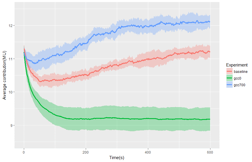
In the first set of experiments, from the baseline experiment, numbers of GCC and CC are varied to create two experiments: gcc0 and gcc700. The gcc0 experiment has no GCC and 700 CCs; while gcc700 has 700 GCCs and no CC. Figure 7 compares the contribution of the baseline, gcc0, and gcc700 experiments. In the baseline experiment, the number of CCs was 300 and the number of GCCs was 400, the contribution had a drop at the beginning but gradually increase; but it was still lower than the initial contribution. In gcc0 experiment with no GCC, the average contribution dropped down and reached the equilibrium. If the number of GCCs was increased to 700 then the contribution went over the initial value at time 0. The first conclusion is that the presence of GCCs can significantly increase the average contribution in the whole population.

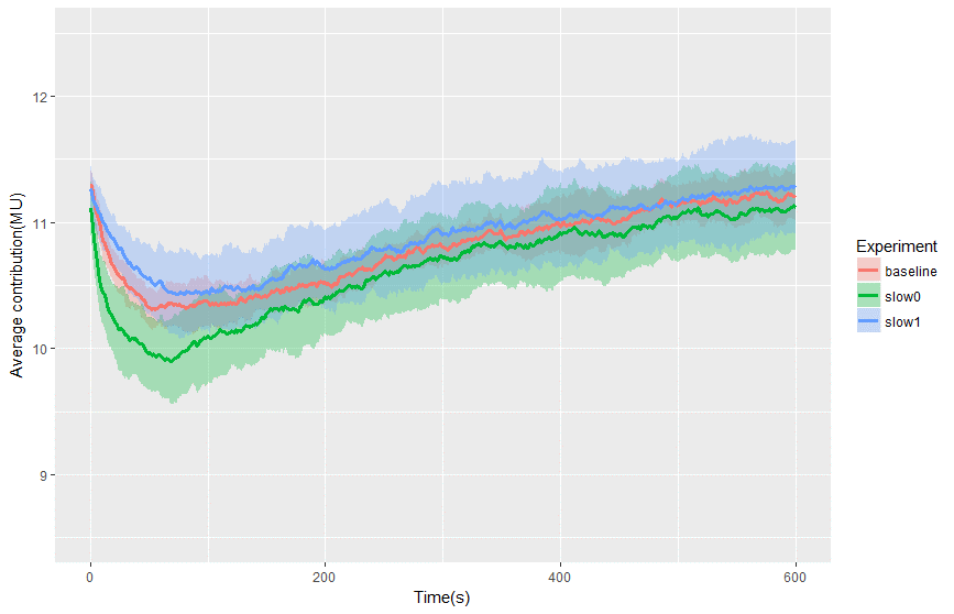
In the second set of experiments, the contribution when we changed the percentage of slow GCC to 0 (everybody evaluates 30 times per minute) and to 1 (everybody evaluates 5 times per minute). Figure 8 shows the contribution of the baseline, slow0, and slow1 experiments. The contribution has the same trend with minimal decrease/increase in value. Thus, it can be concluded that the evaluation speed does not have a significant effect on the average contribution.

Lastly, the third set of experiments varied the number of people stay generous longer by setting percentageLongerStayGenerous to 0 (stay0) and 1 (stay1). In the stay1 experiment, all agents stay generous longer, i.e. evaluate whether to stop being generous 5 times per minutes. On the other hand, in the stay0 experiment, all agents stay generous shorter, i.e. evaluate whether to stop being generous 30 times per minutes. Figure 9 compares the average contribution of the baseline, stay0, and stay1 experiments. All three experiments have the same trending. The contribution drop at the beginning, but always increased later, even in the case all GCCs being less generous. The conclusion from this last set of experiment is that the more generous the GCCs were, the faster the contribution increased.

A closer look within groups

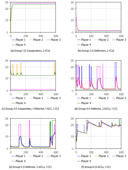
To explain the effect of GCCs, an analysis of the contribution dynamics within groups is needed. Figure 10 presents contribution dynamics within six groups that are chosen from the simulation runs. The x-axis is time in seconds and the y-axis shows the contribution. Different groups have different combinations of player types. Groups 1 and 2 have no GCCs. Group 1 has more cooperators so the contribution is high; Group 2 has more defectors so the contribution is low. When GCCs are introduced into the game, we have Groups 3, 4, 5, and 6.

The GCC behaviour of pulsing causes the average contribution of the game to increase. For example, in Groups 3 and 4, the contribution is increasing within the game but dropping down after GCCs get out of Generous state. Within the Generous state, other CCs and GCCs increase their contribution slowly (depending on the learning rate of the belief update function) but then drop down when GCCs go down. However, in some situations, the contribution keeps at a high level, such as in Groups 5 and 6. Especially when comparing Groups 4 and 6, they have the same type structure but, in the end, the contribution of Group 6 is higher. This is because the green player made two pulses in a short amount of time and the second pulse has a longer duration, which allows other GCCs and CCs to increase their contribution to a higher level. These groups demonstrate how the presence of GCCs can increase the overall contribution which is the conclusion of Section 3.29.

Discussion

The continuous-time PGG

The new preference type GCC has explained some group dynamics in the continuous-time setting. Even though GCCs boost contribution in overall, there are some group compositions that break down the contribution such as when there are many defectors in a group. There are two situations that can lead to a high contribution. The first is a group combination of only Cooperators and CCs/GCCs. But since Cooperators are few in the population, there are not many of these groups. The second case is the GCCs pulse at the same time or sequentially. This requires the group to have at least two GCCs and some form of pulse-related cooperation. If the communication is limited, achieving mutual cooperation is possible but hard in continuous-time PGG. Nevertheless, these interesting interactions have shown that the continuous-time PGG with flow payoff can trigger a different mode of reasoning compared to discrete time.

The reasons for a different reasoning mode can be that continuous time allows participants to change their contribution immediately when an event happens and express their intention. For example, in a group where everyone is contributing, when a participant free rides, other members can react immediately and drop their contribution to 0 in order to show that they are not happy with the free riding behaviour. However, afterwards, even though the free riders later increase contribution, the group can still fail to reach full cooperation because of trust issues. Another possible reason for different reasoning is that it is relatively cheap to pulse because of the flow payoff. The pulse can be seen as the participant pays a small amount to signal their good-will to contribute. Pulsing behaviour does not strongly affect the contribution because its intention is unclear to others and people may be waiting for others to act first.

Lastly, since the number of participants playing the no-communication continuous-time setting is only 20 in the experiment of Oprea et al. (2014), many assumptions have been made during the data analysis of this case study. For example, the pulse rate is estimated to be 0.7 per minute. Another example would be that the ratio of agent behavioural types is estimated from only 20 people. Future experiments should be performed with more participants to collect more data on behaviour and increase the accuracy of data analysis.

Uses of the ABOOMS Framework

The main purpose of the ABOOMS framework is to provide a unified development methodology for the ABMS community. The central idea is that by following activities in the framework modellers can practise the object-oriented mindset. Even though the framework focuses on the development process of agent-based models, the simulation model that is designed with the framework will have good documentation as a co-product since UML diagrams are used throughout the framework, from analysis to design and implementation. Although ABMS research has increasingly agreed to adopt OOAD to design and implement their models, UML is not mentioned much in their publications (Bersini 2012). Bersini (2012) has made an effort to introduce some UML diagrams (class, sequence, state and activity diagrams) to the ABMS community. Our work is not to compete but to extend this effort by demonstrating the application of OOAD mindset and UML specification. Good documentation increases model reproducibility and concept/component reusability. The framework also facilitates better communication and serve as a bridge between disciplines.

Indeed, there are other works that focus on the documentation of agent-based models. One example is the ODD (Overview, Design concepts, and Details) protocol that is first developed by Grimm & Railsback (2006) then improved by Grimm et al. (2010). The primary objective of the ODD protocol is to standardize the descriptions of agent-based models by providing a common format that is complete, understandable, and reproducible. To use the ODD protocol, modellers fill in information following a given sequence of seven elements, grouped in three categories (overview, design concepts, and details). The ODD protocol is not designed to support the development process; however, it is a good tool to describe an already-implemented agent-based simulation. It might be a good idea to use the ABOOMS framework in combination with the ODD protocol: the modellers can use the framework for development, then integrate the information created with the ABOOMS framework with the ODD protocol for model description and publication.

In term of flexibility, the ABOOMS framework provides a loose structure which leaves room for other practices and tools to be incorporated. For example, modellers can apply other proposed system structures when identifying agents in the Analysis process, e.g. the structure consisting of active and passive agents by Li (2013). Another example is that the modellers have the flexibility to implement concepts from different theories in the Design process such as different classes for emotions, learning, etc. Modellers can also design different classes for various methods of agent reasoning such as fuzzy system, genetic algorithm, and neural network.

Lastly, the framework is designed to be easy to use by providing details on both the macro and micro level of the development process. And modellers can also practise the object-oriented mindset just by following the detailed tasks listed in the micro process. This also ensures that the key SE principle of separation of concerns is properly applied. The general idea is that the system is broken into layers and components that each has specific concerns and responsibilities with as little overlap as possible. This reduces the complex system into a series of manageable components. Therefore, the system is easy to change, since a change of a feature is usually isolated to a single component (or a few components directly associated with that feature), instead of interlaced throughout a large and complex code base. However, the framework does require modellers to have a basic knowledge of UML, not all the diagrams, but at least the five useful ones that are introduced and mentioned in this paper (use case diagram, class diagram, statechart, sequence diagram, and activity diagram). When having enough experience, people can start to apply advanced SE concept such as design patterns when utilising the framework.

In summary, in the context of the increasing complexity of simulation models, it can be difficult to control and manage projects without SE methods. Impromptu development approaches can result in simulations with inflexible design, insufficient testing, and ambiguous documentation. Using the ABOOMS framework or other SE methods leads to the benefits of identifying correct requirements to implement the simulation that meets the modellers’ needs. By identifying the necessary features and designing a good model, the development cost is optimised and it also reduces the post-development cost like maintenance or continuous improvement.

Conclusion and Future Works

In this paper, we showcased the ABOOMS framework and its capabilities by picking specifically a case study of continuous game PGGs, highlighting how the framework handles it. In the case study, participants can contribute asynchronously and we observed from laboratory data that the reasoning mode in continuous time is different from discrete time. This was leading to the need for new social reference types (Wary Cooperator, Generous Conditional Cooperators) and pulsing behaviour to model the continuous-time PGG. The simulation showed that even though pulsing behaviour is not an effective way to communicate cooperation intention, it can raise the average contribution in certain settings: the ratio of participants with pulsing behaviour or the timing of these pulses. The continuous-time setting is challenging because it creates a higher level of complexity and generates behaviour that is not present in discrete time. The ABOOMS framework, especially with the support of statecharts, allows modellers to easily describe and model asynchronous behaviour in such a dynamic environment.

Overall, we demonstrated that the ABOOMS framework can act as general guidance for applying OOAD to modelling social agents in PGGs. Firstly, the framework as a complementary approach enhances the design of agent-based models in the sense of reusability and extensibility. Because of the SE principle of separation of concerns, it is easier to reuse a part of a model in another, assemble parts from multiple models to construct a new one, or extending a part of the model without affecting other functionalities. Secondly, the framework improves the communication between different stakeholders (e.g. economists, ecologists, psychologists, and computer scientists) working jointly on a case study. This work is meant to be the first step to overcome the communication barrier between the different stakeholders, to achieve a standard agent technology with integrated interdisciplinary foundation.

While the framework worked well for the test case, there are some limitations with the current version of the framework. So far the framework has only been tested for one type of PGGs and other types might require an alteration of utility functions or gameplay structure. Some ideas would include spatial PGG in which agent locations affect its access to resources or PGG with variant incomes. It could also be tested for related games such as Prisoner’s Dilemma and Common Pool Resources. Another limitation is that, since the UML diagrams are highly recommended in the framework, researchers need to acquired essential background knowledge to utilise UML diagrams for the simulation development process. A start can be made by reading Bersini's excellent "UML for ABM" paper (Bersini 2012) and for a more in depth coverage we recommend Martin Fowler's book "UML Distilled" (Fowler 2004).

For the future work, more laboratory experiments of continuous-time PGGs are required to confirm the existence of the pulsing behaviour and proposed social preference types. Further investigation on other behavioural aspects such as learning or sanction behaviours in continuous time compared to discrete time is needed as well. Finally, we believe that besides Economics, the framework could also find its use in related disciplines which use the ABMS as a research tool, such as Ecology or Sociology. We therefore encourage scholars from these disciplines to be adventurous and give it a try.

References

AMIN, E., Abouelela, M. & Soliman, A. (2018). The Role of Heterogeneity and the Dynamics of Voluntary Contributions to Public Goods: An Experimental and Agent-Based Simulation Analysis. Journal of Artificial Societies and Social Simulation 21 (1), 3: https://www.jasss.org/21/1/3.html. [doi:10.18564/jasss.3585]

BERGIN, J. & MacLeod, W. B. (1993). Continuous Time Repeated Games. International Economic Review, 34(1), 21.

BERSINI, H. (2012). UML for ABM. Journal of Artificial Societies and Social Simulation, 15(1), 9: https://www.jasss.org/15/1/9.html. [doi:10.18564/jasss.1897]

BOOCH, G. (2007). Objected-Oriented Analysis and Design with Applications. Upper Saddle River, NJ: Addison-Wesley.

COLLINS, A., Petty, M., Vernon-Bido, D. & Sherfey, S. (2015). A Call to Arms: Standards for Agent-Based Modeling and Simulation. Journal of Artificial Societies and Social Simulation, 18(3), 12: https://www.jasss.org/18/3/12.html. [doi:10.18564/jasss.2838]

DEITEL, P. & Deitel, H. (2007). Java How to Program. Upper Saddle River, NJ: Prentice Hall Press.

DORSEY, R. E. (1992). The voluntary contributions mechanism with real time revisions. Public Choice, 73(3), 261– 282. [doi:10.1007/BF00140922]

ELSENBROICH, C. & Gilbert, N. (2014). ‘Agent-Based Modelling.’ In Modelling Norms. Berlin Heidelberg: Springer, pp. 65-84.

FEHR, E. & Gächter, S. (2002). Altruistic punishment in humans. Nature, 415(6868), 137-40. [doi:10.1038/415137a]

FISCHBACHER, U., Gächter, S. & Fehr, E. (2001). Are people conditionally cooperative? Evidence from a public goods experiment. Economics Letters, 71(3), 397-404.

FOWLER, M., Kobryn, C., & Scott, K. (2004). UML Distilled: A Brief Guide to the Standard Object Modeling Language. Reading, MA: Addison-Wesley Professional.

FRIEDMAN, D. & Oprea, R. (2012). A continuous dilemma. American Economic Review, 102(1), 337-363.

GRAHAM, I., O’Callaghan, A. & Wills, A. C. (2000). Object Oriented Methods: Principles & Practice. Reading, MA: Addison-Wesley.

GRIMM, V., Berger, U., DeAngelis, D. L., Polhill, J. G., Giske, J. & Railsback, S. F. (2010). The ODD protocol: A review and first update. Ecological Modelling, 221(23), 2760-2768.

GRIMM, V. & Railsback, S. F. (2006). Agent-based models in ecology: patterns and alternative theories of adaptive behaviour. In F. C. Billari, T. Fent, A. Prskawetz & J. Sche_ran (Eds.), Agent-Based Computational Modelling. Heidelberg: Physica-Verlag, pp. 139-152. [doi:10.1007/3-7908-1721-X_7]

LARAKI, R., Solan, E. & Vieille, N. (2005). Continuous-time games of timing. Journal of Economic Theory, 120(2), 206-238.

LI, X. (2013). Standardization for Agent-based Modeling in Economics. Available at: http://mpra.ub.uni-muenchen.de/54284/.

LUCAS, P., de Oliveira, A. C. M. & Banuri, S. (2014). The Effects of Group Composition and Social Preference Heterogeneity in a Public Goods Game: An Agent-Based Simulation. Journal of Artificial Societies and Social Simulation, 17(3), 5: https://www.jasss.org/17/3/5.html.

MACAL, C. M. & North, M. J. (2010). Tutorial on agent-based modelling and simulation. Journal of Simulation, 4(3), 151-162. [doi:10.1057/jos.2010.3]

NEYMAN, A. (2012). Continuous-time Stochastic Games. Games and Economic Behavior, 104, 92-130.

NORTH, M. J. & Macal, C. M. (2007). Managing Business Complexity: Discovering Strategic Solutions with Agent-Based Modeling and Simulation. Oxford: Oxford University Press. [doi:10.1093/acprof:oso/9780195172119.001.0001]

OPREA, R., Charness, G. & Friedman, D. (2014). Continuous time and communication in a public-goods experiment. Journal of Economic Behavior and Organization, 108, 212-223.

ROSSITER, S. (2015). Simulation Design: Trans-Paradigm Best-Practice from Software Engineering. Journal of Artificial Societies and Social Simulation, 18(3), 9. [doi:10.18564/jasss.2842]

SANNIKOV, Y. (2007). Games with Imperfectly Observable Actions in Continuous Time. Econometrica, 75(5), 1285–1329.

SIEBERS, P.-O. & Davidsson, P. (2015). Engineering Agent-Based Social Simulations: An Introduction. Journal of Artificial Societies and Social Simulation , 18(3), 13: https://www.jasss.org/18/3/13.html. [doi:10.18564/jasss.2835]

SIMON, L. K. & Stinchcombe, M. B. (1989). Extensive Form Games in Continuous Time: Pure Strategies. Econometrica, 57(5), 1171.

THE ANYLOGIC COMPANY (2018). AnyLogic. Available at: https://www.anylogic.com/.

VU, T. M. (2017) A software engineering approach for agent-based modelling and simulation of public goods games. PhD thesis, University of Nottingham.

VU, T. M. (2018). An Agent-Based Simulation of Continuous-Time Public Goods Games. CoMSES Computational Model Library. Retrieved from: https://www.comses.net/codebases/ee195d48-802b-4ca1-a4a5-314e3c670a6d/.