Catch Me if You Can: Using a Threshold Model to Simulate Support for Presidential Candidates in the Invisible Primary

Introduction

When Donald Trump descended the elevators in Trump Tower in June, 2015 to announce his candidacy for the Republican Party nomination for president, few pundits gave him much of a chance of winning the party primary, much less the general election. But shortly after his entrance in the race, he jumped into the polling lead (Schleifer 2015) and dominated media coverage of the race (Patterson 2016). Trump was able to parlay this consistent edge in support during the invisible primary - the time between when people announce their candidacy and when the first votes are cast in the first state (Iowa) - into securing the nomination.

On one hand, Trump’s ability to win the nomination was not surprising given his level of support in the invisible primary. Candidates with higher polling numbers during the invisible primary are more likely to win the nomination (Adkins & Dowdle 2005; Dowdle, Adkins, & Steger 2008; Steger 2009, 2008; Donovan & Hunsaker 2009). Furthermore, a lead in the polls often aligns with a significant amount of media coverage. While Steger (2015) notes that the media does not tell people what to think, it does influence what primary voters think about. Although media attention may not directly factor into who wins a nomination (Steger 2007), other scholars note that it can indirectly influence the contest through fundraising during the invisible primary (Mutz 1995; Damore 1997).

On the other hand, many scholars and data journalists were skeptical of Trump’s chances of winning the 2016 Republican Party nomination because they predicted that party elites would rally against him by endorsing another candidate (Cohn 2015; Bycoffee 2015; Prokop 2015; Sides 2015). Winning endorsements is important because it signals to donors, party activists, and party organizers that a particular candidate is both viable and preferred by the party elite (Cohen et al. 2008). While receiving endorsements can help a candidate win the nomination (Summary 2010; Steger 2007; Whitby 2014), Steger (2015) notes that party officials should be generally unified in order to maximize this effect.

These scholars make it clear that where candidates stand at the end of the invisible primary is important for understanding which candidates win the major parties’ presidential nominations. As such, it is worthwhile to explore how candidates gain an edge during this critical time period, particularly since there is a high level of volatility in the public’s candidate preferences during presidential primaries, in part due to shifts in public attention from one candidate to another (Steger 2008). While some scholars explore which factors impact the length of a candidacy and include the invisible primary in their analysis (e.g. Shen 2008; Norrander 2006), the preponderance of the presidential primary literature focuses on the nomination outcome.

The nature of the invisible primary is such that conducting simulations can be helpful. First, primary elections lack the traditional partisan cues that are present in general elections, leaving voters to rely on other mechanisms to decide on which candidate to support such as candidate characteristics (e.g., Jackman & Vavreck 2010; Norrander 1986; Campbell 1983), ideology (e.g., Wattier 1983; Bartels 1988), issues (e.g., Bartels 1985), viability (e.g., Abramson 1992; Collingwood, Barreto, & Donovan 2012; Bartels 1989), or some combination thereof (e.g., Stone, Rapoport, & Abramowitz 1992; Abramowitz 1989). Second, no actual voting occurs during the invisible primary, making it difficult for candidates to create momentum surrounding their campaigns (e.g., Steger 2007; Norpoth & Perkins 2011; Adkins & Dowdle 2001).

In this manuscript, we utilize an interdisciplinary approach that uses a threshold model of social interaction with a political outcome: which candidate wins at least a plurality of support at the end of the invisible primary. To do this, we conduct a network analysis simulation using three candidates while varying the size of the primary electorate. Such analyses are not unprecedented when exploring election dynamics (e.g., Lou et al. 2014) but we have not seen many models that include flexibility of supporter intensity (though Rolfe 2013, models unconditional cooperators in her models of voting turnout) and the existence of decay.

We find that frontrunners are more likely to lead at the end of the invisible primary than non-frontrunners, but only under certain conditions. Specifically, there are three components to a candidate holding the lead prior to the Iowa caucuses: a sizeable lead in the polls at the onset of the race, an environment in which there is little information decay, and an unwavering base of support. The absence of any of these factors can lead at least a plurality of voters to be undecided thus creating uncertainty as to who will win the nomination. These results suggest that campaigns must use tools to keep their supporters informed and strengthen their allegiance to the candidate.

Public attention and networks

Campaigns are “attempts by competing partisan elites to reach citizens with political communications and persuade them to a point of view” (Zaller 1992 p. 215). However, the transmission of these communications is mediated by social factors and influence (Lazarsfeld 1944; Berelson et al. 1954). Thus, although most communications are elite initiated, the dynamics of mass communication deserve attention as well.

Recently, Swearingen, Stiles & Finneran (2019) posited that the analysis of primary campaigns relies excessively upon elite-level variables and found that a mass component called public attention (Ripberger 2011) is important in predicting primary results. Public attention can be understood as the result of information flows through individuals’ networks. Individuals are organized into social networks with ongoing patterns of relationship with other members (Granovetter 1973; Granovetter 1978) that “encourage some views and opinions while discouraging others” (Huckfeldt 1995). The decisions of most actors are conditional on the behavior of others and people tend to care more about the actions and opinions of those closer to them (Hu et al. 2014; Siegel 2013; Rolfe 2013; Siegel 2009).

An individual’s position in a network, the size of their network (Rolfe 2013; Siegel 2009) and consequent types of information flows has been found to have an array of economic (Rolfe 2013; Granovetter 1978), social (Takacs 2001) and political consequences. Most relevant here, Berelson et al. (1954) find that being subject to conflicting information makes people less likely to vote, a finding supported in more recent analysis as well (Santoro & Beck 2018; Siegel 2013).

Network dynamics are also important in adoption of complex communication or behaviors. However, complex communication may require reinforcement from more than one source for adoption. As opposed to simple communication (e.g. When is the bus coming? Who won the game last night?), complex communication includes complying with a cultural norm or practice or adopting contentious communication or participating in collective action (Centola & Macy 2007). Romero et al. (2011) find evidence that simple and complex communication display distinct communication patterns across networks and that political communication is typical of complex communication. Whereas simple communication travels more quickly through loose ties, the same is not necessarily true of complex communication because it requires reinforcement, which is more likely in more tightly clustered groups (Centola & Macy 2007). Thus, social diffusion of complex communication is highest at moderate to high levels of structural consolidation (Centola 2015). Actually, casting a vote for one primary candidate vs. another is a behavior rather than only an adoption of complex communication. Centola (2010) finds that adoption of behaviors is much more likely in a lattice network, where reinforcement is common, than in other types of networks, which may have many loose ties.

Supporting the notion of a political campaign as complex communication, Romero et al. (2011) find significant differences based on content in the way messages on Twitter diffuse. Relative to other types of content, political messages have a higher “stickiness,” which is the probability of adoption after one or more exposures. They also find that political messages have higher “persistence,” which is the extent to which repeated exposures continue to have significant marginal effects in probability of adoption. The transmission of political and other kinds of potentially controversial information through a network may also subject it to selective disclosure (Cowan & Baldassarri, 2018) where members of networks do not express disagreement with an idea but only agreement. Collective action is also less likely if networks connected by information and connective technology (ICT) is not strong ( Hu et al. 2014).

Threshold model

We posit that a type of social contagion model called a threshold model (Granovetter 1978) explains levels of public attention. In this model, each actor displays inertia but will act after his or her threshold (number or proportion of others who first make a similar decision) has been reached (Watts 2002). For example, a primary voter may be willing to vote for a candidate only if he or she knows at least two people who will vote for that candidate. In this example, the voter’s threshold for that candidate is two. This primary voter may have different thresholds for different candidates and a different primary voter may have a different threshold for each candidate.

A threshold model allows a focus not only on individuals and their preferences but also on how those individuals interact and how preferences aggregate (Granovetter 1973). Such a model also fits well with dynamics of mass political information and voting behavior. Voters possess variable but on average low amounts of poorly integrated political information (see, for example, Carpini & Keeter 1996 or for a more current example Bowyer et al. 2017). As a consequence, the typical voter has little ability to absorb, integrate or resist political messages (Zaller 1992). Adoption of political messaging, then, becomes a matter of repeated exposure. Although individuals vary in their susceptibility to influence based on political knowledge and their values driven dispositions, more exposure increases the likelihood of adoption.

The exposure must be reinforced, however, or a decay process sets in wherein people forget the messages they have adopted unless they have heard them recently (Zaller 1992). Thus, exposure to political messages immediately prior to a campaign should figure most prominently in spurring voting (Centola & Macy 2007). Further, the process of decay may cause an unraveling of support across the network. If one actor in the network fails to regularly communicate a political message, then those other actors whose thresholds have been reached in part by the first actor may not support the candidate any longer and so on.

Threshold Models and Primaries

In this section, we explain why our model is suited for the primary election context. To that end, our model is appropriate for the specific contexts of primaries as elections with low structure, low salience, and low information, characteristics often exacerbated by multiple candidates and lengthy campaigns. Because of these features, the activated networks tend to be of small size but higher impact because of low likelihood of exit and more diversity of messages. We explain these unique factors of primaries and their effects on networks below.

A threshold model is especially useful in analyzing situations “where many actors behave in ways contingent on one another, where there are few institutionalized precedents and little preexisting structure” (Granovetter 1978). Primaries fit this description well, as they are low salience campaigns with low amounts of information and messaging where party labels cannot provide a heuristic for vote choice.

Elections, general or primary, “involve equal members of a generic, loose-knit community” (Rolfe 2013, p. 94). However, there are also some key differences between the two types of elections.People tend to organize themselves into homophilous networks, meaning they connect themselves to people similar to themselves (Santoro & Beck 2018; Hu et al. 2015; Macy 2007). There is evidence that the two major American political parties have unique social networks (Grossman & Dominguez 2009). This does not mean that the structures are inherently different; rather, they have separate constituencies and coalitions. Primaries are an interesting case in that, because of lower salience, we would not ordinarily expect primary voters to select only other network members who agree with their primary candidate preferences. In other words, they have selected into party networks based on the general election not for a primary. Similarly, network exit based on different primary candidate preferences is unlikely.

There is also an interaction between salience and size of the relevant network. In less salient elections, the number of relevant actors in a member’s network is smaller than in more salient elections. Candidates and supporters have less incentive to reach out and campaign as hard and so network members are less likely to be exposed to new messages. Thus, in selecting a candidate, voters are more likely to rely on the opinions of their family members and perhaps a close friend or two (Rolfe 2013).

Due to the low information available in a primary, we also expect networks to be more influential during primaries than during general elections. Consequently, network members are less able to resist campaign messages (Zaller 1992). Since network members are not exiting (because they are in the network because they are homophilous with respect to partisan preferences) and since they are less able to resist the messages they do receive (due to low information), they will continually receive high impact messages from their networks. Thus, we reason that networks during primaries provide a potent mechanism for persuasion.

As another consequence of members not opting out of networks with diverse messages, they are more likely to encounter them in the primaries than in the general election. General election vote choice literature that finds that network members exposed to diverse communication are more likely to change their minds than those exposed only to repeated similar messages although possibly less likely to be able to decide (Santoro & Beck 2018). As a result, loyal supporters or unconditional actors (those who support a candidate regardless of the messaging around them) may be critical to primary success. The percentage of unconditional actors in a network is critical to vote turnout (Rolfe 2013) and we expect that factor to be important in primary success as well.

Another important difference between general elections and primary elections is that in the United States, general elections generally provide a binary choice to voters (voter turnout is also a binary choice) while primary voters often must select from several candidates. Models based on binary opinion such as the threshold q-voter model (Vieira & Anteneodo 2018) may serve better to emulate general election behavior. Another binary variant is the consensus model, where opinions are real numbers between 0 and 1 and an agent takes the average of compatible neighbors having a difference of opinion less than some threshold value. Fortunato relates the convergence threshold to the behavior of the average degree of the social graph as the population increases (Fortunato 2005). Lou et al. (2014) note the importance of creating a model that can account both for multiple candidates and for heterogeneity in individual preferences. By allowing for multiple candidates within the same network, our model is suited for a primary election rather than a general election with two major party candidates. To date the literature describing threshold models for diffusion in a voter network with multiple candidates often concentrates on the Influence Maximization Problem – that is, how to select the necessary seeds at the beginning in order to get a maximum of the voters to prefer one candidate over the others. For example, see Lu, Fan et al. (2014) or Kim, Beznosov et al. (2015). While this information would doubtless be very useful, we see our contribution as a logically prior step to maximizing influence.

Finally, the presidential primary process is much longer and drawn out than its general election counterpart. Major candidates routinely announce their candidacies 10-12 months prior to the Iowa caucuses and in upwards of 18-20 months before the major party nomination conventions. By comparison, the general election formally kicks off (per Federal Election Commission finance regulations) after the conventions, leaving roughly 3-4 months of campaigning. This is important for our decay parameter, as the primary’s drawn-out process is more relevant for this context. While this model may be modified for a general election context, its current specification is better suited for the longer, slower-paced invisible primary.

Theory and model expectations

Based on the above discussion, we derive the following expectations. Elites direct primary campaigns and other types of political campaigns at individuals in an attempt to persuade them to adopt the elites’ messages. Primary voters are situated variably within communication networks, which act as a filter upon the type and amount of information they receive. Each person in the network has a threshold for each primary candidate, which is determined by his political information, awareness and values. The level of political information across voters varies but is on average quite low. Thus, most voters are unable to resist a campaign message when it has reached a certain threshold (which varies stochastically across voters). Some voters will have a very low adoption threshold for one candidate and a very high threshold for other candidates (i.e. true believers).

When a voter’s threshold has been reached for a candidate, he becomes persuaded by that candidate. He signals his support to others in his network which counts towards reaching the threshold of his neighbors. Because of the process of decay described above, however, the message he receives from his neighbors must be reinforced or his threshold may no longer be met and he may withdraw support. This loss of support could cause cascading decreases in support among his neighbors if their thresholds are no longer met. Thus, a true believer, though in the minority of cases, is quite valuable to a candidate because he or she can both spread support and resist effects of decay.

We explicate the following model expectations (E1-6):

• E1: Ceteris paribus, the initial frontrunner is more likely to win the simulated invisible primary than other candidates.
• E2: As the size of the initial lead between the frontrunner and runners-up decreases, undecided voters are more likely to become a plurality of the invisible primary electorate.
• E3: As a candidate’s proportion of true believers increases, that candidate is more likely to win the simulated invisible primary.
• E4: (a) As a candidate’s proportion of true believers decreases, the proportion of undecideds increases. (b) This relationship will be more pronounced under conditions of decay.
• E5: Under conditions of no decay, the frontrunner is more likely to win the simulated invisible primary than under conditions of decay.
• E6: As decay increases, the likelihood that the frontrunner wins the simulated invisible primary decreases.

Methods

In this section, we describe the underlying algorithm for the Threshold Network Diffusion Model (see model and output data at https://github.com/lseiter/threshold-model). This model consists of a network of voters with various threshold levels for the candidates, and an iterative sequence of preference matrices, which record the preferred candidates for the voters per iteration. The preferred candidate for each voter is determined by the percentages of support that the voter’s neighbors have for each candidate in comparison with the voter’s threshold levels.

Definition and initialization of elements of the threshold network diffusion model

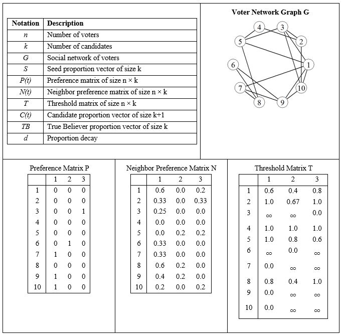
The model begins with \(n\) voters deciding on \(k\) candidates. The voters are put in arbitrary order from \(1,…,n\). The candidates are also put in arbitrary order and assigned numbers from \(1, …, k\). The voters influence each other's preferences via social relationships which we represent by a simple, connected, undirected graph \(G\), such as one given in Figure 1 below. Each node represents a voter; each edge connecting two nodes represents an influencing relationship between the corresponding voters. Two nodes connected by an edge are called "neighbors."

Preference matrix

After each iteration of the simulation, a voter will either prefer exactly one candidate over all of the others or have no preference. We record the preferred candidate of each voter at time \(t\) as a time-dependent \(n \times k\) matrix, \(P(t)\). The entries are all 0 or 1. Namely, if Voter \(i\) prefers Candidate \(\alpha\) over all of the others after the t_th iteration of the model, then \(P_{i\alpha}(t)=1\). Otherwise \(P_{i\alpha}(t)=0\). Voter \(i\) is "undecided"' if \(P_{i\alpha}(t)=0\) for all candidates \(\alpha = 1,\dots, k\). In Figure 1, the preference matrix indicates that Voters 7, 9 and 10 prefer candidate 1, while voter 6 prefers candidate 2 and voter 3 prefers candidate 3. The remaining voters are undecided.

The initial preference matrix \(P(0)\) begins with all rows being 0, except for the rows of a certain, randomly chosen set of voters called seeds. The proportion of seeds among the voters is recorded as a vector of size \(k\), \(S = (s_1,\dots,s_k)\). For each \(\alpha=1,\dots, k,\) the value \(s_{\alpha}\) represents the proportion of voters in the network that start with a preference for Candidate \(\alpha\). The seeds will be randomly chosen from the graph. In Figure 1, the Seed Vector is given as \(S = (0.3,0.1,0.1)\). The 30% initially supporting Candidate 1 were chosen to be Voters 7, 9, and 10; the 10% for Candidate 2 was Voter 6; and Voter 3 was the sole seed for Candidate 3.

Neighbor preference matrix

Voters’ preferences are determined by those of their neighbors. For each voter, we record the proportion of neighbors who prefer each of the candidates. Specifically, for each \(i = 1,\dots,n\) and \(\alpha = 1,\dots,k\), we define \(N_{i\alpha}(t)\) to be the proportion of the neighbors of Voter \(i\) who prefer Candidate \(\alpha\) after the \(\it{t}^{th}\) iteration of simulation.

The graph in Figure 1 shows Voter 1 has neighbors 3, 5, 7, 9 and 10. The Neighbor Preference Matrix \(N\) indicates 60% of Voter 1's neighbors support Candidate 1 (Voters 7, 9 and 10), while 20% support Candidate 3 (Voter 3). The rest are undecided. Note also that some voters, such as Voter 4, are surrounded completely by undecided voters. Hence, Row 4 will consist of all 0's.

Threshold matrix

Each voter requires a certain proportion of neighbors in order to prefer a given candidate. This proportion is called the threshold level. We put the various threshold levels together as a matrix \(T\). Specifically, to prefer Candidate \(\alpha\), Voter \(i\) needs at least \(T_{i\alpha}\) of its total neighbors to prefer Candidate \(\alpha\). If multiple thresholds are met, the preference will be given to the candidate with the smallest threshold, or a random pick in the event of a tie.

Note: Either \(0\leq T_{i\alpha}\leq 1\) or \(T = \infty\). If \(T_{i\alpha} = 0\), then Voter \(i\) will always prefer Candidate \(\alpha\). If \(T_{i\alpha}=1\), then Voter \(i\) will prefer Candidate \(\alpha\) only if all neighbors prefer Candidate \(\alpha\). If \(T_{i\alpha}=\infty\), then Voter \(i\) will never prefer Candidate \(\alpha\).

The threshold values for the voter network are determined as follows. First, using the proportions given by the Seed Vector , the seeds for each candidate are randomly chosen among the voters. If Voter \(i\) is a seed for Candidate \(\alpha\), then we set \(T_{i\alpha}=0\) and \(T_{i\beta}=\infty\) for all \(\beta \neq \alpha\). Second, the threshold values of the non-seeds are randomly determined from a range between \(2 / d_i\) and 1, where \(d_i\) is the number of neighbors of Voter \(i\) in the network. As a consequence and consistent with the dynamics of complex communication discussed in the literature review, at least two neighbors must support a particular candidate before a node can change preferences. The values of the resulting \(n \times k\) matrix \(T=(T_{i\alpha})\) never change during the run of the simulation.

In Figure 1, the threshold levels for Voter 8 are 0.8, 0.4, 1.0 for Candidates 1, 2 and 3, respectively. Voter preference is assigned based on the lowest threshold that is met. This means that if 40% of Voter 8's neighbors support Candidate 2, then Voter 8 will support Candidate 2. However, if the 40% threshold for Candidate 2 is not met, the next highest threshold of 80% for Candidate 1 will be checked. Finally, all of Voter 8's neighbors need to support Candidate 3 for Voter 8 to support Candidate 3.

Since Voters 7, 9 and 10 are seeds for Candidate 1, the corresponding rows in threshold matrix T contain 0 in column 1, indicating this set of voters does not require any neighbors to convince them to retain their candidate preference, while the value ∞ indicates they will never switch to Candidate 2 or 3 regardless of neighbor preference.

Voter preference update

The simulation is recursive with respect to time \(t\). We define the current Neighbor Preference Matrix \(N(t)\) by using the neighbor proportions generated from the previous Voter Preference Matrix \(P(t-1)\). Then we generate the current Voter Preference Matrix \(P(t)\) by comparing the proportions in the current Neighbor Preference Matrix \(N(t)\) with the levels given in the Threshold Matrix \(T\). The general schematic of the simulation can be visualized as the following functional dependencies.

$$ P(\textit{previous})\mapsto N(\textit{current})\\ (N(\textit{current}),T)\mapsto P(\textit{current})$$

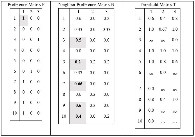
In our example (Figure 1), the proportion of Voter 1’s neighbors that prefer Candidate 1 (60%) meets the minimum threshold for Candidate 1 (60%). Since none of Voter 1’s neighbors prefer Candidate 2, the 40% threshold is not met. Similarly, the 20% that prefer Candidate 3 fail to meet the 80% threshold. Thus, after the first iteration of the simulation, the initially undecided Voter 1 will set their preference to Candidate 1. This update is reflected in the voter preference matrix P of Figure 2. The other undecided voters have not met their thresholds and thus remain undecided. The updated neighbor preference matrix is shown in Figure 2.

Convergence of voter preference

The iterations continue until convergence of some sort occurs. After each iteration, we compile the results in a vector \(C\) of size \(k+1\), each of the first \(k\) entries being the proportion of voters preferring the corresponding candidate and the last entry being the proportion of undecided voters. The simulation ends when the distance between current and previous preference proportions reaches some minimal value.

After the first iteration, 40% of voters prefer Candidate 1, while Candidates 2 and 3 both maintain their original 10%. The remaining 40% of voters are undecided. The updated voter preference proportion vector is thus (0.4, 0.1, 0.1, 0.4), with the fourth value being the undecided vote.

Initial results

The model was tested with graphs of various size and structure. Figure 3 presents the result of 100 random small world graphs. Small world networks exhibit short distances between nodes and high transitivity or clustering, which many real world networks also display (Watts & Strogatz 1998). In Figure 3, the small world graph has size 1000, with each node connected by default to its nearest 6 neighbors, and a 10% probability of a neighboring edge being rewired to a random node. The seed proportion for candidates 2 and 3 was held constant at 10% each, while the proportion for candidate 1 ranged from 22.5 to 32.5%, with increments of 2.5%.

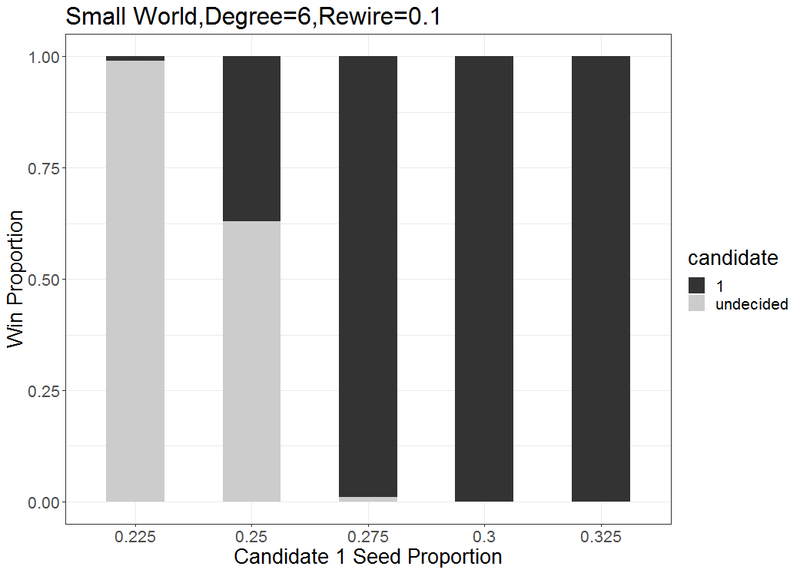
As Figure 3 indicates, all simulations ended with either a majority of undecided voters or with Candidate 1 – the initially leading candidate – winning. This finding provides preliminary evidence for our first expectation, holding the proportion of True Believers constant and randomizing social network changes, that, the candidate with the initial lead is more likely to win the invisible primary than other candidates. The seed proportion appears to have a significant role to play in the final outcome of the race. Namely, if the proportion of seeds for Candidate 1 is high enough, then all else equal, Candidate 1 is sure to win the election. On the other hand, if Candidate 1's seeds are proportionally low, then Candidate 1 will fare no better than the other candidates and the race will end with mostly undecided voters. According to these results, the bifurcation proportion value for Candidate 1 seems to reside somewhere between 0.25 and 0.275. This finding supports our second expectation that as the size of the initial lead decreases, undecided voters are more likely to constitute a plurality of the electorate.

Note that the results in Figure 3 are based on a threshold proportion for non-seed voters that ranges between \(2/d_i\) and 1, where \(d_i\) is the degree of Voter \(i\) in the network. Thus, a minimum of 2 neighbors must prefer a given candidate, which is consistent with the characteristics of complex communication discussed above. If the minimum proportion is reduced to \(1/d_i\), the seed bifurcation for Candidate 1 decreases significantly to approximately 0.175 for the same small world graph configuration.

Model extension: True believer proportion

The model described above assumes that all seeds for the candidates are what we call true believers, that is, they start preferring one candidate and will never waver from this position. In order to see if the seed proportion alone accounted for the final result of the election, we adjusted the model so that some of the seeds would not necessarily be true believers.

This model extension differentiates between candidate seeds who are considered true believers and those considered adherents. Both share the same initial candidate preference in voter preference matrix P; however, the threshold value for their preferred candidate will differ. A true believer’s threshold is set such that their candidate preference will never change, while an adherent’s threshold allows a change in candidate preference.

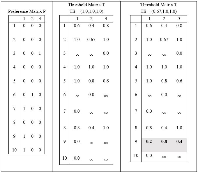
In addition to seed vector \(S\), the threshold matrix is initially generated based on the proportions specified in a true believer vector \(TB = (tb_1,\dots, tb_k)\). Each \(tb_{\alpha}\) represents the proportion of seed voters \(s_{\alpha}\) that are true believers of Candidate \(\alpha\), while \((1-tb_{\alpha})\) represents the proportion of adherents. The voter preference matrix \(P(0)\) is generated from the seed vector following the original algorithm. However, we need to adapt how values in threshold matrix \(T(0)\) are generated for candidate seeds. If Voter \(i\) is a true believer for Candidate \(\alpha\), then \(T(0)_{i\alpha}=0\) and all other elements in row \(i\) are set to \(\infty\) as in the original algorithm. If Voter \(i\) is an adherent for Candidate \(\alpha\), then a random set of threshold values are generated, with \(T_{i\alpha}\) assigned to the minimum value in the set. An adherent thus has a threshold \(>\)0 that must be met to retain their initial preference for Candidate \(\alpha\).

\(TB\) = (1.0, 1.0, 1.0) indicate 100% of candidate seeds are true believers. However, \(TB\) = (0.67, 1.0, 1.0), implies 67% of candidate 1 seeds are true believers, with the remaining seeds deemed adherents. The example preference matrix P in Figure 4 shows three seeds for candidate 1 (Voters 7, 9 and 10), thus two are randomly chosen as true believers (7, 10). The adherent voter 9 is assigned a threshold >0 for their preferred candidate.

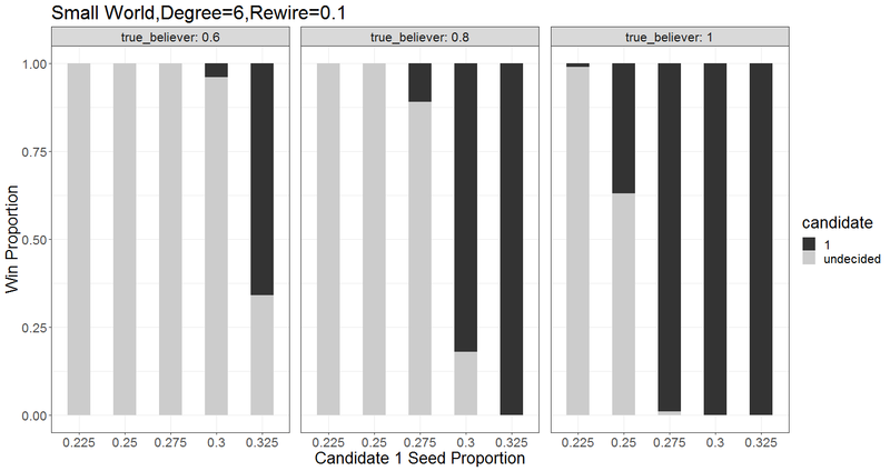
Figure 5 shows the impact of the true believer proportion on voter preference for Candidate 1, while candidates 2 and 3 were held constant at 1.0. Note that the rightmost facet with true_believer = 1.0 corresponds to Figure 3, the default when we assume each seed is a true believer.

We see that, if we lower the proportion of true believers among the seeds, the overall outcome of the campaign gets increasingly hazy, ending often in a majority of undecided voters. This is striking in the rightmost facet, which corresponds to starting the campaign season with a high proportion of Candidate 1 seeds. When all of the seeds are true believers, the campaign ends with an easy victory for Candidate 1 when the seed proportion is sufficiently high. But, when only 60% of those seeds are true believers, then most of the campaign simulations end with a majority of undecided voters.

These findings support expectation 3 (as a candidate’s proportion of true believers increases, he or she is more likely to win the simulated invisible primary) although we only test the expectation for Candidate 1. They also support expectation 4(a)-- as a candidate’s proportion of true believers decreases, the proportion of undecideds increases. In some ways, the 2016 Democratic primary helps illustrate the evidence in support of expectation 3. Pollsters do not generally ask respondents if they are true believers, but they do gauge a respondent's level of enthusiasm. As Bump (2016) shows, there was a correlation between enthusiasm and support during the early 2016 primaries. Interestingly, it was Hillary Clinton whose supporters were more enthusiastic about their candidate of choice. While this is not conclusive evidence, it helps to shed some light on how increasing a candidate’s share of true believers can enhance his/her likelihood of winning.

Similarly, comparing results along the rows shows us the impact of the different proportions of seeds when the true believers are held constant. As might be expected, the results indicate that, if either the seed proportions within the overall population or the true believer proportions within the seeds are too meager, the election will not converge to a solid lead for any of the candidates.

Intriguingly, there is indication that the seed ratios have more impact than the true believer ratios. The middle facet shows the results for the case where the seed proportion for Candidate 1 is 30% of the entire voter population but the true population among these seeds is relatively low (only 80% of these seeds are true believers). The proportion 0.8 \(\times\) 0.30=0.24 of seeds are true believers and will never waver away from their support of Candidate 1. As the figure shows, voters choose Candidate 1 over 80% of the time.

We compare this scenario with the results of the rightmost facet (true believer proportion is 1.0), which involves the situation where the seed proportion for Candidate 1 is slightly smaller (0.25) but consists entirely of true believers. For this scenario, the overall results are less likely to be positive for Candidate 1. Very few of the simulations end with a Candidate 1 victory. Thus, we see that a comparatively large population of true believers does not make up for a relatively small group of initial supporters. This is perhaps best illustrated by Ron Paul’s candidacy for the 2012 Republican Party nomination. A Public Policy Polling survey in December, 2011, just weeks before the Iowa caucuses, asked how committed a respondent was to their top candidate choice. Although Paul placed a distant third place behind Mitt Romney and Newt Gingrich, his supporters were the most committed to his candidacy: 50 percent were strongly committed to him, compared to 41 percent of Romney supporters and 39 percent of Gingrich supporters. Ultimately, Paul ended up finishing fourth in popular vote (RealClearPolitics, 2012a) and third in the delegate count (RealClearPolitics 2012b).

Model extension: Decay

By default, each voter is weighted equally in computing the neighbor preference matrix \(N\). The final adaption of the model involves decay in voter influence, which is achieved by modifying voter weight. A voter has a default weight of 1. Thus, all neighbor preferences are equal in determining whether a given candidate threshold is met. A subset of voters is randomly chosen at each time interval, with each voter in the subset assigned a random weight in the range of 0.5 to 0.9. The lower voter weight results in smaller proportions in the neighbor preference matrix, making it more difficult for candidate thresholds to be met.

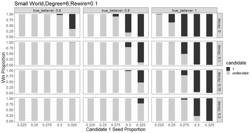
Figure 6 shows the results when decay is introduced into the model. Note that the top row in Figure 6 is the same as the plot from Figure 5, corresponding to no decay. The role of decay is clearly prominent according to these results. In all cases, the presence of decay greatly increases the probability that the election will not converge to a clear winner.

Generally then, the frontrunner is more likely to win the elections when no decay is incorporated. This finding supports expectation 5, that under conditions of no decay, the frontrunner is more likely to win the simulated invisible primary than under conditions of decay. As decay increases, the likelihood that the frontrunner wins decreases (expectation 6). Further, a smaller proportion of true believers under conditions of decay is even more likely to result in a plurality of undecideds than under conditions of no decay. This finding supports expectation 4(b), that a decrease in the proportion of true believers is associated with an increase in the proportions of undecideds and that the relationship will be more pronounced under conditions of decay.

Based on previous research, we can expect decay to be a real, prominent fixture in invisible primaries. We see this primarily in studies about television ads, which can have a strong initial impact in voters’ minds, although these effects dissipate over time (Alan S. Gerber & Dowling 1996; Sides & Vavreck 2013; Hill et al. 2013; and Huber & Arceneaux 2007). If such findings can be generalized to most/all campaign information dissemination, there is plenty of room for uncertainty in an invisible primary. This uncertainty can provide an opening for candidates who are not the front-runner.

Graph Variation

As discussed in the literature review, network structure can impact results. To examine the effects of our model in different structures still consistent with elections as involving “equal members of a generic, loose-knit community” (Rolfe 2013, p. 94) we used Small World graphs with varying degree and rewiring probability, as well as scale free Barabasi-Albert graphs of varying growth factor, with 100 graphs of size 1000 generated per configuration. Figure 7 contains the proportion of simulations that result in a win for Candidate 1 for each graph configuration. The Small World graphs having degree 6, along with the Barabasi-Albert graph (growth factor m=3, average degree 5.98) outperform the graphs with degree 4, including the Barabasi-Albert (m=2, degree 3.97).

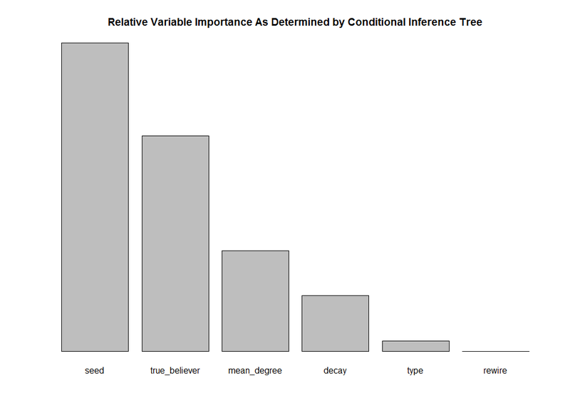
While graph configuration has some impact on the outcome, the differences are not as significant as those related to seed and true believer proportion. Figure 8 shows the relative variable importance determined through the construction of a conditional inference tree, with Seed and True Believer proportion being the most important predictors of outcome, while graph type and rewiring probability, which affects the mean distance between nodes, being the least important.

Discussion

In this paper, we developed and ran a series of simulations based on the literature about the invisible primary and using a threshold type of network model. Simulations are particularly useful in studying the invisible primary because of the difficulty of testing hypotheses using polling data. Through the simulations, we find three components that are important to a candidate holding the lead prior to the Iowa caucuses. First and intuitively, a sizeable lead in the polls (i.e. seed proportion) at the outset of the race is critical. In our models, the battle is not between the first place and second place candidates. Rather, it is between the first place candidate and the undecideds. Thus, for the candidate doing the best in the polls, it is his or her race to lose. More specifically, we find that when the frontrunner polls above 30%, it is much more certain that she will maintain her standing going into the Iowa caucus.

The second component that affects the lead candidate’s chances is an unwavering base of support (i.e., how true are the true believers). Our results show that as the proportion of true believers decreases for the candidate, his or her chances of being overcome by an undecided electorate increases. This result sheds light on why some frontrunners are able to maintain their lead while others are unable to convince the electorate to continue supporting them. While our initial model showed that gaining 30% of the lead in the polls is sufficient for the lead candidate to win, that finding was contingent upon very sticky support. As the true believers decreases to 60% of the candidate’s support, it is overwhelmingly likely that the electorate will remain undecided.

The third component that is critical to frontrunner success is little to no information decay. When we relax the assumption that nodes (i.e., voters) will automatically communicate their preferences to their neighbors, the front runner’s chances again diminish. Candidate communications may lapse or voters could become inattentive for a variety of reasons. Even when the lead candidate is polling at 30% and has an unwavering base of support, decay at a level of 0.2 (which we can interpret as neighbors not sending or receiving information 20% of the time) affects the front runner’s chances of holding on.

The absence of any of these factors can lead at least a plurality of voters to be undecided thus creating uncertainty as to who will win the nomination. This uncertainty impacts the race; it can encourage more candidates to enter (e.g., as in the Republican Party in 2016) or it can lead to elites withholding endorsements. These results suggest that campaigns must do whatever they can to keep their supporters informed and strengthen their allegiance to the candidates.

Conclusion and Future Research

The importance of a polling lead, an unwavering base and full information transmission has been demonstrated in this paper. What we have demonstrated is not how a candidate can be upset by another candidate, but the conditions under which a plurality of the primary electorate will remain undecided, creating favorable conditions for a political upset to occur.

Nonetheless, the results of our model do have empirical referents. Between late August and mid-December of 2015, Donald Trump generally ranged from about 22-30% in the polls. During this time, other candidates such as Ben Carson and Carly Fiorina saw their own support surge. Once Carson’s support began dropping, however, Trump surpassed the 30% level, sustaining his lead until the end of the invisible primary (Real Clear Politics 2016). This finding suggests that Trump’s level of support, coupled with the large field, was significant in cementing his status as the winner of the invisible primary despite his lack of endorsements and fundraising prowess.

Future work should incorporate exogenous shocks into the model. It is our hunch that under the conditions we have established, that a shock could tip the balance from the front runner to a different candidate. In the invisible primary, examples of shocks include debate performances, fundraising reports, endorsements or scandals. During the primary phase, this would also include election outcomes in various states.

References

ABRAMOWITZ, A. I. (1989). Viability, Electability, and Candidate Choice in a Presidential Primary Election: A Test of Competing Models. The Journal of Politics, 51, (4), 977-992 [doi:10.2307/2131544]

ABRAMSON, P. R., Aldrich, J. H., Paolino, P., & Rohde, D. W. (1992). “Sophisticated” Voting in the 1988 Presidential Primaries. The American Political Science Review, 86(1), 55-59. [doi:10.2307/1964015]

ADKINS, R. E., & Dowdle, A. J. (2001). How Important Are Iowa and New Hampshire to Winning Post-Reform Presidential Nominations? Political Research Quarterly, 54(2), 431–444. [doi:10.1177/106591290105400210]

ADKINS, R. E., & Dowdle, A. J. (2005). Do Early Birds Get the Worm? Improving Timeliness of Presidential Nomination Forecasts. Presidential Studies Quarterly, 35(4), 646–660. [doi:10.1111/j.1741-5705.2005.00270.x]

ALAN S. Gerber, D. D., Gregory A. Huber & Dowling, C. M. (1996). The big five personality traits in the political arena. Annual Review of Political Science, 14, 265–287. [doi:10.1146/annurev-polisci-051010-111659]

BARTELS, L. M. (1985). Expectations and Preferences in Presidential Nominating Campaigns. American Political Science Review, 79(03), 804–815. [doi:10.2307/1956845]

BARTELS, L. M. (1988). Presidential Primaries and the Dynamics of Public Choice. Princeton, N.J: Princeton University Press.

BARTELS, L. M. (1989). 'After Iowa: Momentum in Presidential Primaries.' In The Iowa Caucuses and the Presidential Nominating Process. Boulder: Westview Press, pp. 121–148. [doi:10.4324/9780429311987-5]

BERELSON, B., Lazarsfeld, P., & McPhee, W. (1954). Voting: A Study of Opinion Formation in a Presidential Election. Chicago: University of Chicago Press.

BOWYER, B. T., Kahne, J. E., & Middaugh, E. (2017). Youth comprehension of political messages in YouTube videos. New Media & Society, 19(4), 522–541. [doi:10.1177/1461444815611593]

BUMP, P. (2016). Bernie sanders’s supporters are passionate — But maybe not as much as you think. Washington Post, February 20. Retrieved from: https://www.washingtonpost.com/news/the-fix/wp/2016/02/20/bernie-sanderss-supporters-are-passionate-but-maybe-not-as-much-as-you-think/.

BYCOFFEE, A. (2015). The endorsement primary. Retrieved from: http://projects.fivethirtyeight.com/2016-endorsement-primary/.

CAMPBELL, J. E. (1983). Candidate Image Evaluations: Influence and Rationalization in Presidential Primaries. American Politics Research, 11(3), 293–313. [doi:10.1177/004478083011003002]

CARPINI, M. X. D., & Keeter, S. (1996). What Americans Know about Politics and Why It Matters. Yale: Yale University Press.

CENTOLA, D. (2010). The spread of behavior in an online social network experiment. Science, 329(5996), 1194–1197. [doi:10.1126/science.1185231]

CENTOLA, D. (2015). The Social Origins of Networks and Diffusion. American Journal of Sociology, 120(5), 1295–1338. [doi:10.1086/681275]

CENTOLA, D., González-Avella, J. C., Eguíluz, V. & San Miguel, M. (2007). Homophily, cultural drift, and the coevolution of cultural groups. Journal of Conflict Resolution, 51(6), 905–929. [doi:10.1177/0022002707307632]

Centola, D., & Macy, M. W. (2007). Complex Contagions and the Weakness of Long Ties. American Journal of Sociology, 113(3), 702–34. [doi:10.1086/521848]

COHEN, M., Karol, D., Noel, H., & Zaller, J. (2008). The Party Decides: Presidential Nominations Before and After Reform. Chicago, IL: University of Chicago Press. [doi:10.7208/chicago/9780226112381.001.0001]

COHN, N. (2015). Donald Trump vs. the party: Why he’s still such a long shot. Retrieved October 6, 2015, from: http://www.nytimes.com/2015/09/10/upshot/donald-trump-vs-the-party-why-hes-still-such-a-long-shot.html?_r=0.

COLLINGWOOD, L., Barreto, M. A., & Donovan, T. (2012). Early primaries, viability and changing preferences for presidential candidates. Presidential Studies Quarterly, 42(2), 231–255. [doi:10.1111/j.1741-5705.2012.03964.x]

COWAN, S. K., & Baldassarri, D. (2018). “It could turn ugly”: Selective disclosure of attitudes in political discussion networks. Social Networks, 52, 1-17. [doi:10.1016/j.socnet.2017.04.002]

DAMORE, D. F. (1997). A Dynamic Model of Candidate Fundraising: The Case of Presidential Nomination Campaigns. Political Research Quarterly, 50(2), 343–364. [doi:10.2307/448961]

DONOVAN, T., & Hunsaker, R. (2009). Beyond Expectations: Effects of Early Elections in U.S. Presidential Nomination Contests. PS: Political Science & Politics, 42(1), 45-52. [doi:10.1017/s1049096509090040]

DOWDLE, A. J., Adkins, R. E., & Steger, W. P. (2008). The viability primary: Modeling candidate support before the primaries. Political Research Quarterly, 62(1), 77–91. [doi:10.1177/1065912908317032]

FORTUNATO, S. (2005). On the consensus threshold for the opinion dynamics of Krause–Hegselmann. International Journal of Modern Physics C, 16(02), 259-270. [doi:10.1142/s0129183105007078]

GRANOVETTER, M. S. (1978). Threshold Models of Collective Behavior. American Journal of Sociology, 83(6), 1420–1443. [doi:10.1086/226707]

GRANOVETTER, M. S. (1973). The Strength of Weak Ties. American Journal of Sociology, 78(6), 1360–1380. [doi:10.1086/225469]

GROSSMANN, M., & Dominguez, C. B. K. (2009). Party Coalitions and Interest Group Networks. American Politics Research, 37(5), 767–800 [doi:10.1177/1532673X08329464]

HILL, S. J., Lo, J., Vavreck, L., & Zaller, J. (2013). How Quickly We Forget: The Duration of Persuasion Effects From Mass Communication. Political Communication, 30(4), 521–547. [doi:10.1080/10584609.2013.828143]

HU, H. H., Cui, W. T., Lin, J., & Qian, Y. J. (2014). ICTs, social connectivity, and collective action: A cultural-political perspective. Journal of Artificial Societies and Social Simulation, 17(2), 7. https://www.jasss.org/17/2/7.html. [doi:10.18564/jasss.2486]

HU, X. & Keller, N. (2015). Agent-based modeling and simulation of child maltreatment and child maltreatment prevention. Journal of Artificial Societies and Social Simulation, 18(3), 6: https://www.jasss.org/18/3/6.html. [doi:10.18564/jasss.2783]

HUBER, G. A. & Arceneaux, K. (2007). Identifying the persuasive effects of presidential advertising. American Journal of Political Science, 51(4), 957–977. [doi:10.1111/j.1540-5907.2007.00291.x]

HUCKFELDT, R. R., & Sprague, J. (1995). Citizens, Politics and Social Communication: Information and Influence in an Election Campaign. New York: Cambridge University Press.

JACKMAN, S., & Vavreck, L. (2010). Primary politics: race, gender, and age in the 2008 democratic primary. Journal of Elections, Public Opinion and Parties, 20(2), 153–186. [doi:10.1080/17457281003697156]

KIM, H., Beznosov, K., & Yoneki, E. (2015). A study on the influential neighbors to maximize information diffusion in online social networks. Computational Social Networks, 2(1), 3. [doi:10.1186/s40649-015-0013-8]

LAZARSFELD, P., Berelson, B., & Gaudet, H. (1944). The People’s Choice. New York, NY: Duell, Sloan & Pearce.

LOU, J.-K., Wang, F.-M., Tsai, C.-H., Hung, S.-C., Kung, P.-H., Lin, S.-D., Chen, K.-T. & Lei, C.-L. (2014). A social diffusion model with an application on election simulation. The Scientific World Journal, 2014, 14. [doi:10.1155/2014/180590]

LU, Z., Fan, L., Wu, W., Thuraisingham, B., & Yang, K. (2014). Efficient influence spread estimation for influence maximization under the linear threshold model. Computational Social Networks, 1, 2. [doi:10.1186/s40649-014-0002-3]

MUTZ, D. C. (1995). Effects of Horse-Race Coverage on Campaign Coffers: Strategic Contributing in Presidential Primaries. The Journal of Politics, 57(4), 1015-1042. [doi:10.2307/2960400]

NORPOTH, H., & Perkins, D. F. (2011). War and Momentum: The 2008 Presidential Nominations. PS: Political Science & Politics, 44(3), 536–543. [doi:10.1017/s1049096511000631]

NORRANDER, B. (1986). Correlates of vote choice in the 1980 presidential primaries. The Journal of Politics, 48(1), 156–166. [doi:10.2307/2130931]

NORRANDER, B. (2006). The attrition game: Initial resources, initial contests and the exit of candidates during the US presidential primary season. British Journal of Political Science, 36(3), 487–507. [doi:10.1017/s0007123406000251]

PATTERSON, T. E. (2016). Pre-Primary News Coverage of the 2016 Presidential Race: Trump’s Rise, Sanders’ Emergence, Clinton’s Struggle. Cambridge, MA: Harvard University Press [doi:10.2139/ssrn.2798258]

PROKOP, A. (2015). Political scientists think “The Party” will stop Trump. They shouldn’t be so sure. Retrieved October 6, 2015, from: http://www.vox.com/2015/9/23/9352273/party-decides-trump-sanders.

REALCLEARPOLITICS (2012a). 2012 Republican Delegates. Retrieved March 28, 2018, from: https://www.realclearpolitics.com/epolls/2012/president/republican_delegate_count.html.

REALCLEARPOLITICS (2012b). 2012 Republican popular vote. Retrieved March 28, 2018, from: https://www.realclearpolitics.com/epolls/2012/president/republican_vote_count.html.

REALCLEARPOLITICS (2016). 2016 Republican Presidential Nomination. Retrieved March 28, 2018, from: https://www.realclearpolitics.com/epolls/2016/president/us/2016_republican_presidential_nomination-3823.html.

RIPBERGER, J. T. (2011). Capturing curiosity: Using internet search trends to measure public attentiveness. Policy Studies Journal, 39(2), 239–259. [doi:10.1111/j.1541-0072.2011.00406.x]

ROLFE, M. (2013). Voter Turnout: A Social Theory of Political Participation. New York, NY: Cambridge University Press.

ROMERO, D. M., Meeder, B. and Kleinberg, J. (2011). Differences in the Mechanics of Information Diffusion Across Topics: Idioms, Political Hashtags, and Complex Contagion on Twitter. Proceedings of the 20th International Conference on World Wide Web, (pp. 695–704). New York, NY. [doi:10.1145/1963405.1963503]

SANTORO, L. R., & Beck, P. A. (2018). 'Social Networks and Vote Choice.' In The Oxford Handbook of Political Networks. Oxford: Oxford University, pp. 383–406. [doi:10.1093/oxfordhb/9780190228217.013.40]

SCHLEIFER, T. (2015). Donald Trump leads new national poll. CNN. Retrieved from: http://www.cnn.com/2015/07/14/politics/donald-trump-leading-poll/index.html.

SHEN, F. (2008). Staying alive: The impact of media momentum on candidacy attrition in the 1980-2004 primaries. The International Journal of Press/Politics, 13(4), 429–450.

SIDES, J. (2015). The unsettled, uncertain, undecided Republican presidential primary (in one graph). Retrieved August 15, 2017, from: https://www.washingtonpost.com/news/monkey-cage/wp/2015/07/08/the-unsettled-uncertain-undecided-republican-presidential-primary-in-one-graph/?utm_term=.61ca7e8ce818.

SIDES, J., & Vavreck, L. (2013). The gamble: Choice and chance in the 2012 election. Retrieved March 28, 2018, from: https://press.princeton.edu/titles/10350.html. [doi:10.1515/9781400852277]

SIEGEL, D. A. (2009). Social Networks and Collective Action. American Journal of Political Science, 53(1), 122–138.

SIEGEL, D. A. (2013). Social networks and the mass media. American Political Science Review, 107(4), 786–805. [doi:10.1017/s0003055413000452]

STEGER, W. P. (2007). Who wins nominations and why?: An updated forecast of the Presidential Primary Vote. Political Research Quarterly, 60(1), 91–99. [doi:10.1177/1065912906298597]

STEGER, W. P. (2008). Forecasting the presidential primary vote: Viability, ideology and momentum. International Journal of Forecasting, 24(2), 193–208. [doi:10.1016/j.ijforecast.2008.02.006]

STEGER, W. P. (2009). Polls and elections: How did the primary vote forecasts fare in 2008? Presidential Studies Quarterly, 39(1), 141–154. [doi:10.1111/j.1741-5705.2008.03663.x]

STEGER, W. P. (2015). A Citizen’s Guide to Presidential Nominations: the Competition for Leadership. New York, NY: Routledge. [doi:10.4324/9780203522486]

STONE, W. J., Rapoport, R. B., & Abramowitz, A. I. (1992). Candidate Support in Presidential Nomination Campaigns: The Case of Iowa in 1984. The Journal of Politics, 54(4), 1074–1097. [doi:10.2307/2132109]

SUMMARY, B. (2010). The endorsement effect: An examination of statewide political endorsements in the 2008 Democratic Caucus and primary season. American Behavioral Scientist, 54(3), 284–297. [doi:10.1177/0002764210381709]

SWEARINGEN, C.D., Stiles, E., & Finneran, K. (2019). Here’s Looking at You: Public Attention in Presidential Primaries. Social Science Quarterly, 100(5), 1777-1792. [doi:10.1111/ssqu.12671]

TAKACS, K. (2001). Structural embeddedness and intergroup conflict. Journal of Conflict Resolution, 45(6), 743–769.

VIEIRA, A. R., & Anteneodo, C. (2018). Threshold q-voter model. Physical Review E, 97(5), 052106.

WATTIER, M. J. (1983). Ideological voting in 1980 Republican presidential primaries. The Journal of Politics, 45(4), 1016-1026. [doi:10.2307/2130423]

WATTS, D. J. (2002). A simple model of global cascades on random networks. Proceedings of the National Academy of Sciences, 99(9), 5766–5771. [doi:10.1073/pnas.082090499]

WATTS, D. J. & Strogatz, S. H. (1998). Collective dynamics of ‘small-world’ networks. Nature, 393(6684), 440. [doi:10.1038/30918]

WHITBY, K. J. (2014). Strategic Decision-Making in Presidential Nominations: When and Why Party Elites Decide to Support a Candidate. Albany, NY: State University of New York Press

ZALLER, J. (1992). The Nature and Origins of Mass Opinion. Cambridge, MA: Cambridge University Press.