
Introduction
Global warming has been a profound indicator of human-induced climate change since the mid-20th century. According to Intergovernmental Panel on Climate Change (IPCC 2014), each of the three decades preceding 2014 has been successively warmer at the Earth's surface than any prior decade since 1850. This has led to extreme heat waves and changes in precipitation pattern occurring more frequently. Numerous evidences led IPCC to conclude that human-induced greenhouse emissions are extremely likely to have been the dominant cause of the observed warming. Scientific estimates differ about the intensity of effects, but as we allow the warming to continue, we are facing the risk of the climate crossing the tipping point where any further changes will be irreversible (Lemoine & Traeger 2014).
In response, governmental bodies and international organisations have started to promote climate change mitigation actions, which involve substantial emissions reduction over the decades succeeding 2014; in addition, ideas regarding geo-engineering (Craig & Burns 2016; Roshan et al 2019) have been introduced. Significant international joint efforts on this matter include the Kyoto Protocol, which was adopted in 1997, the Cancun Agreement, which was established in 2010, and the Paris agreement, ratified in 2015. The latter is effectively replacing the Kyoto Protocol. All movements share the common objective of reducing the carbon footprint of the world. In Paris the participating parties agreed to "Holding the increase in the global average temperature to well below 2°C above pre-industrial levels and pursuing efforts to limit the temperature increase to 1.5°C above pre-industrial levels, recognizing that this would significantly reduce the risks and impacts of climate change" (UN 2015, Article 2a).
The implementation of the required carbon reduction policy to achieve this goal poses huge technological, economic, social and institutional challenges, also not to mention the fact that a lot of the carbon quota has already been released by now (for a lively debate on the topic see CarbonBrief 2018). The dilemma in finding the right balance between environmental and economic sustainability has proven to be a prevalent problem among politicians and policy makers.
Modelling and simulation plays an increasingly significant role in exploratory studies for informing policy makers on climate change mitigation strategies. The growth in computing power allows more comprehensive and sophisticated models to be produced and to be put into use. In fact, the existing literature in the discipline is considerably mature, with robust climate models capable of forecasting the weather down to the granularity of hours. There is also considerable research being done in creating more accurate Integrated Assessment Models (IAMs), which focus on examining the human impacts on climate change. Many popular IAMs, as for example DICE (Nordhaus 1992, 2017), RICE (Nordhaus & Yang 1996), and C-ROADS (Climate Interactive 2016) were created as steady state optimisation models. They are highly aggregated models that focus on the economics of global warming by assessing the costs and benefits of steps towards slowing down global warming. From a technical point of view IAMs typically employ a nested structure of neoclassical production functions to represent the energy-economy system (Fiddaman 1997). The DICE model, for example, comprises a traditional economic sector and a novel climate sector, which form a closed-loop interaction. IAMs hold aggregate views on variables and hence are unable to capture a finer level of details of the underlying system components. This is particularly true for humans, who are the major contributors to the natural level of global warming, and are viewed in these models as an aggregation. In reality, however, humans are independent and discrete beings with diverse behaviours. These optimisation models also neglect the non-linear relationships between humans, which could bring about unpredictable patterns. In addition, the tightly-coupled internal components of the models prevent or discourage dynamic modification to their structure. As such, these models lack flexibility in modelling different levels of aggregation and scalability, which constitute their major limitations, considering that the risks and impacts associated with climate change are unevenly distributed, geographically and demographically. An alternative approach that allows modelling populations as a collection of individual and unevenly distributed entities is Agent Based (AB) modelling, often used in the field of Social Simulation. But simulating a huge number of individuals (e.g. the whole population of a country) quickly becomes an issue, as it requires large amounts of computer memory for storing these entities as individual objects and it slows down simulation model execution drastically as all of these objects need to be checked against each other for updates on a regular basis.
Current IAMs do not reflect well the underlying dynamics and drivers of people's changes in behaviour over time. A more sophisticated consideration of individual differences within the population and their influence on the overall evolution of the system is required, as people are the true drivers of change - the ones that change things (Perez et al. 2017). Our research seeks a novel approach to the design of IAMs by combining the top-down approach used in System Dynamics (SD) modelling, where the overall system behaviour is captured through complex feedback loops, with the bottom-up approach used in AB modelling, where a system is modelled as a collection of autonomous decision-making entities. We aim to drive forward the development of hybrid IAMs by providing ideas for how to implement such models using a multi-method approach.
In this paper we present an innovative concept of a scalable hybrid modelling approach for integrated assessment modelling and then show with an illustrative example how this concept can be applied and what a more sophisticated population model offers in terms of potential insight. We use parts of a well-established SD interpretation of the DICE model, developed by Fiddaman (1997) (which we will refer to as the Fiddaman model in the remainder of the paper) to represent the general environment, including economy and climate. Within this environment we use an AB modelling approach to represent hierarchical social structures as well as groups of individuals that can interact with other groups of individuals and the environment. Finally, we use an SD model to represent a conception of the environment inside a collective conscience of those groups of individuals. The target audience this paper is aimed at are model developers that want to explore new ways of creating IAMs.
When reading this paper, please keep in mind that the focus of this paper is on a methodological advance rather than creating a complex model for predictive purposes. Our illustrative example to demonstrate the application of our conceptual framework takes the settings of the United States (US), a country that contributes to the majority of the global carbon footprints and that is the largest economic power in the world. The model considers the carbon emission dynamics of individual states and its relevant economic impacts on the nation over time.
Background
The need for a methodological advance in Integrated Assessment Modelling
There are several papers discussing the usefulness of IAMs. Moss et al. (2010) stress the need for climate change research and assessment and supports the idea of using IAMs for this purpose, as they "improve the analysis of complex issues, such as the costs, benefits and risks of different policy choices and climate and socioeconomic futures". Metcalf & Stock (2015) provide an overview of the more recent debate on the topic and conclude that "the social cost of carbon must have a numerical value and be associated with numerical measures of uncertainty, and we cannot see how that can be done credibly without sophisticated computer models that incorporate climate and economic considerations, that is, without IAMs". Weyant (2017) argues that much of the uncertainty in the use of IAMs represents less the flaws of the models and more the fundamental uncertainty in scientific and economic knowledge of key model features and inputs. This suggests that there is a need for methodological advance in the way IAMs are designed. Another perspective related to the usefulness of IAMs could be drawn from the statement once made by Box (1979) that "all models are wrong but some are useful". Even though the numerical output IAMs produce might not reflect reality (as the output depends on assumptions, which may not reflect reality) these types of models are useful for providing insight and some stimulation for debates, both things that are important for improving our understanding of climate changes and their economic consequences. In order to support the latter, we introduce a new practice of integrated modelling: combining SD and AB modelling to allow studying the disequilibrium dynamics of the system over time, and adding more opportunities for integrating theoretical and empirical knowledge related to human and social behaviour.
Modelling methods
SD modelling, originally developed by Jay Forrester in the 1950s to help corporate managers improve their understanding of industrial processes is concerned with the non-linear behaviour of complex systems over time (Forrester 1961). It deals with internal feedback loops and time delays that affect the behaviour of the entire system. A system is composed of networks of interconnected components, with their relationships giving rise to the aggregate behaviour of the system. There are two different approaches in use for SD modelling: causal loop diagrams for qualitative modelling and stock and flow diagrams for qualitative and quantitative modelling. The mathematical model behind the SD structure is a system of nonlinear, first-order differential and integral equations (Choopojcharoen & Magzari 2012). SD models seek alternatives to the assumptions of optimisation and equilibrium that are inherent in the traditional IAMs. They focused instead on disequilibrium dynamics and feedback complexity, with behavioural decision rules and explicit stocks and flows of capital, labour, and money. The principal purpose of these models is to identify the structural features that have the greatest implications for policy, and thus are worthy of further pursuit (Fiddaman 1997). For an in depth introduction to SD modelling see Morecroft (2007).
In AB modelling a system is modelled as a collection of autonomous decision-making entities called agents (Kotz & Hiessl 2005). Each agent individually assesses its situation and makes decisions on the basis of a set of rules. In AB modelling we describe the system from the perspective of its constituent units (Bonabeau 2002). Agents are designed to mimic the behaviour of their real-world counterparts. They are discrete entities with a memory and with their own goals and behaviours. They are capable to adapt and to modify their behaviour and they can act proactively (where actions depend on motivations generated from their internal state). An AB model is essentially decentralised; there is no place where global system behaviour is defined. Instead, the individual agents interact with each other and their environment to produce complex collective behaviour patterns, capturing emergent phenomena at system level. AB modelling is well suited to modelling systems with heterogeneous, autonomous and proactive actors. This applies well to human-centred systems (Siebers et al. 2007). The individual agents are not limited to represent individuals within a system but can also be used to represent collectives, as for example households, organisations, or even whole nations. For an in-depth introduction to AB modelling see Gilbert & Troitzsch (2005).
While AB modelling and SD modelling are founded on fundamentally different schools of thought, they still strive for a common goal: studying the leverage points of complex systems (Van Dyke Parunak et al. 1998; Phelan 1999). Despite that, there has been little discussion between the two communities and it is not common practice to combine these simulation methods (Lättilä et al. 2010). But interest is rising. A good indicator for this is the growth of the "hybrid track" of the Winter Simulation Conference (WSC 2015). Some more guidance of when it is useful to combine these methods can be found in Lättilä et al. (2010). There are different ways of combining these two methods. One can have agents in a SD environment but also individual agent decision making driven by a SD model (Van Dyke Parunak et al. 1998; Borshchev 2013). Such a combination of modelling approaches allows identifying the structural as well as behavioural features that have the greatest implications for policy and should specifically be taken into account by policy makers. An example of an application related to the topic of this paper is Shafiei et al. (2013) who use integrated AB and SD modelling to study sustainable mobility. However, we did not find any examples of hybrid IAMs.
Conceptual Framework of a Hybrid IAM
Conceptualisation encompasses defining the purpose of the model and its boundaries as well as identifying key variables and describing the behaviour of the model. While going through the conceptualisation process it is important to keep in mind that a model has to be built at the right level of description for every phenomenon; we should not model all we can but what has an impact on the result, at a level of detail that is sufficient for the purpose at hand (Couclelis 2002). We should aim for transparency in order to increase trust in our models (Axelrod 1997). For our model we use the Fiddaman model as a basis, and add a population consisting of groups of individuals. When it comes to modelling these, we go beyond rationality and bounded rationality and create actors with habits and memory that will influence their response to certain political interventions. These actors also have the ability to learn differently, depending on their experiences and initial habits. In order to support the understanding of the behavioural models described in Section 3.16 to Section 3.24 it might help to have a look at the Appendix where their implementation is shown.
Aim
Our Hybrid Climate Assessment Model (HCAM) concept aims to represent the behaviours of groups of individuals under the influence of climate change and external policy makings. In its current state it supports the development of exploratory models rather than predictive models. Certain sub components (e.g. the behavioural models embedded in the agents) might seem to be conceptualised in a simplistic way, but we were aiming to keep things simple for the sake of transparency. Such sub components can be replaced by more complex variants in the future. As such, the model could serve two purposes: enhancing the general understanding on human-induced climate change and stimulating debates amongst policy makers regarding strategies for tackling climate change.
Feedback structure
In SD models, in order to define the model boundary, one separates the relevant components into two groups: endogenous and exogenous. The components involved in the feedback loops of the system are endogenous whereas those not directly affected by the system are exogenous. In our case some of the endogenous components of standard IAMs become part of the integrated AB model, and can therefore be seen as exogenous components in relation to the SD model, and vice versa. Here we considered our idea of a hybrid model where the population is modelled as a collection of individual agents, which then becomes an exogenous component to the SD model, while the CO2 emissions of those agents are part of the SD model and therefore an endogenous component. Governmental policies are enforced by policy makers at different levels in the hierarchy of the geographic structure (from national to local), and are therefore exogenous to the SD model.
To represent the feedback structure of the HCAM we use sector mapping. This requires dividing the model into smaller sectors with each sector complementing the overall feedback structure of the model. In our case this feedback structure is formed by the coupling between an AB model layer and a SD model layer, as well as the causal links between different sectors. As a basis we have used the sector boundary map presented in Fiddaman (1997), which is based on the DICE model. Because our focus is on transparency, we have reduced Fiddaman's original sector boundary map, making sure that our resulting boundary map still follows the principle IAM schematic presented in Metcalf (2015). However, it has reduced complexity due to a reduction in scope and level of detail. We have added an AB model layer to make it a hybrid sector boundary map. Figure 1 illustrates the sector boundaries in the feedback structure of our HCAM and clarifies the distinction between the AB and the SD model layers.
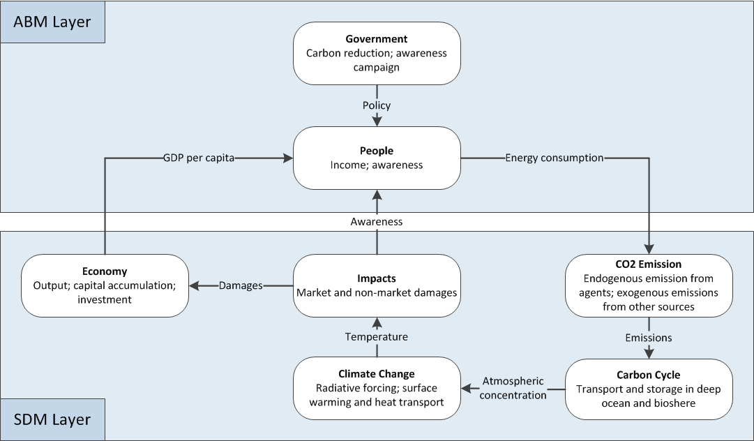
The sectors of Economy, CO2 Emissions, Carbon Cycle and Climate Change, which are generally members of the climate-economy system, make up the portion of the feedback structure in the SD model layer, while the autonomous and decision-making entities, such as People and Government, belong to the AB model layer. The crossing of the AB-SD model boundary occurs when the economic outputs in the SD model layer are distributed to the people in the form of income. The consumption of the people in the AB model layer is driven by their income levels and their consumptions produce emissions. These emissions flow back into the SD model layer and trigger a series of feedback processes, which result in temperature rise. This rise in temperature creates negative Impacts on the economy through climate change damages, resulting in reduced economic output. Furthermore, changes in temperature will trigger the awareness level of the people concerning climate change. The awareness level of the people plays an important role in determining their emission rates. An assumption has been made that emissions choices do not directly influence economic output. In reality the choice of an agent to be environmentally friendly may come at economic cost, resulting in a less crisp AB-SD model boundary.
Base model
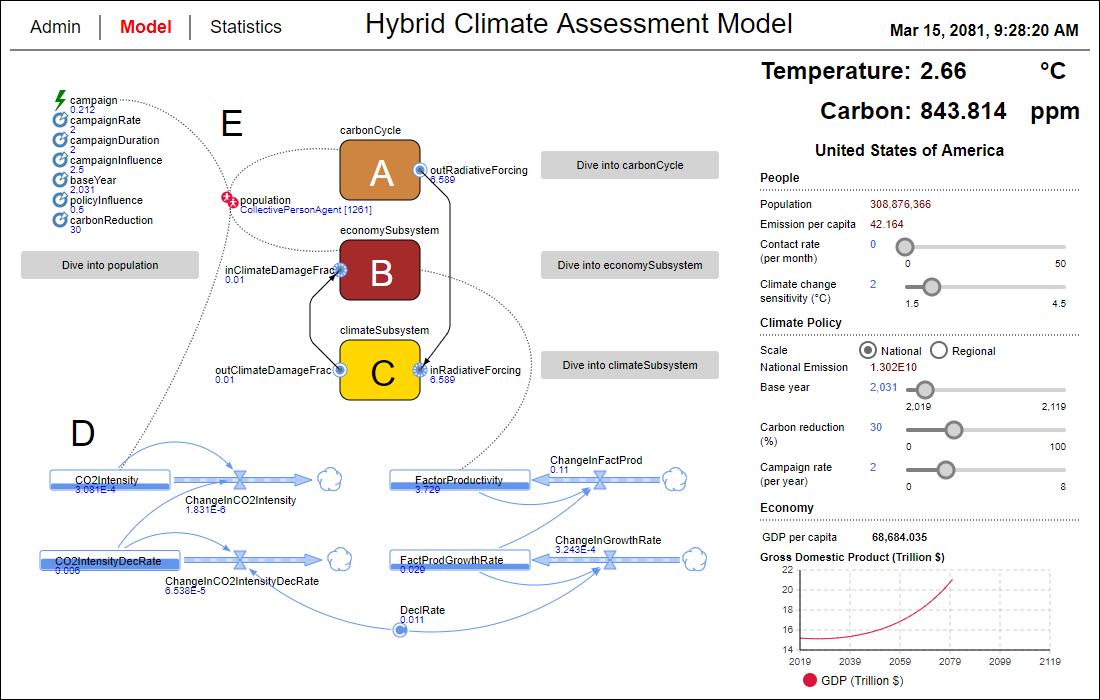
The HCAM incorporates a simplified version of the coupled Climate-Economy SD model described in Fiddaman (1997), who utilised the DICE model developed by Nordhaus (1992) for his model. Equations presented in this section are based on Fiddaman (1997). Figure 2 depicts the overall causal structure of the HCAM in form of a stock and flow diagram. The original Population stock has been replaced by a composite variable Population[..] for storing a disaggregated collection of agents and the government is represented as an autonomous decision-making entity that influences peoples' behaviour through governmental policies.
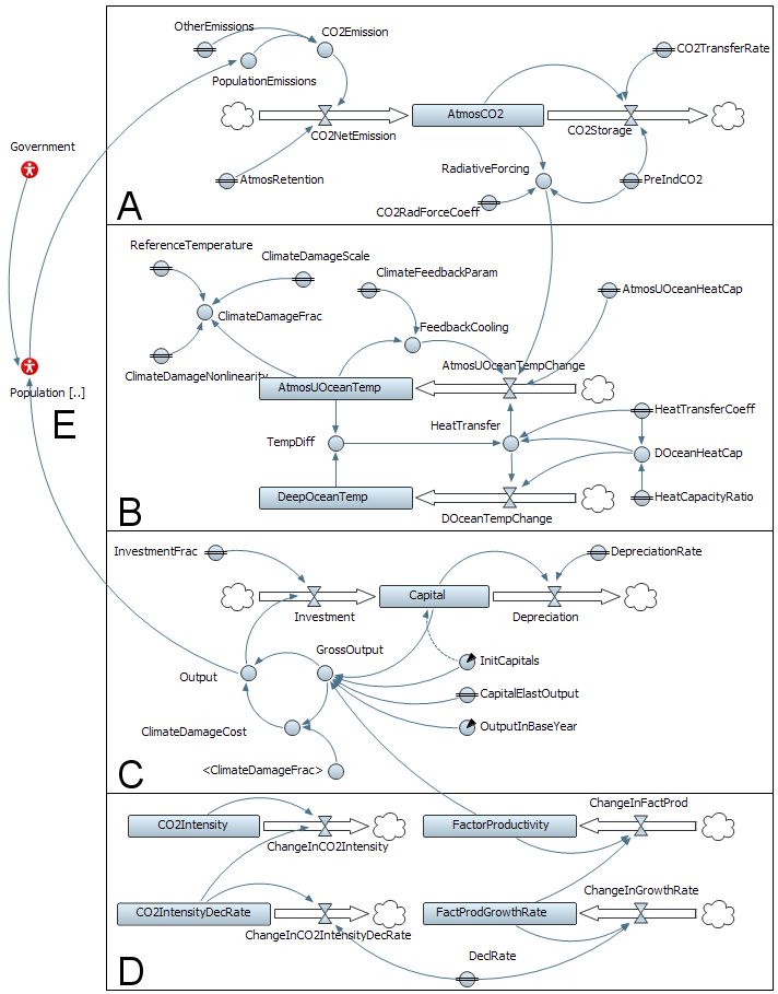
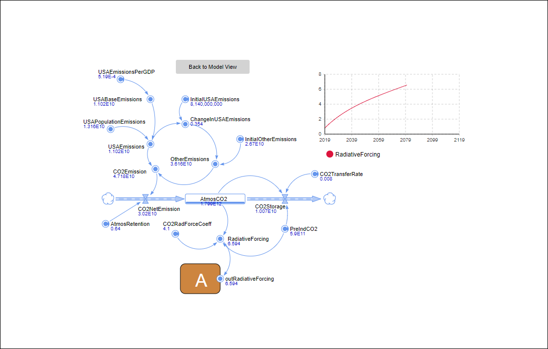
The Carbon Cycle (box A in Figure 2) is a segment of the natural system, which links human economic activities with climate change. Here atmospheric CO2 accumulates with inflows of CO2 emissions and outflows of CO2 to the natural carbon sink. As the HCAM grants users the autonomy of climate policy control, the emissions-control rate is excluded from the feedback loop of the carbon cycle. Instead, it is introduced as an exogenous user input variable. Moreover, as the atmospheric carbon dioxide is simulated at a global scale, the inflows of emissions must represent that of the entire world in order to balance the equation. Hence, we have two variables which amount to the total world emissions: PopulationEmissions and OtherEmissions. PopulationEmissions is a control variable which contains the aggregate emissions of the total agent population (which can represent a subset of the world population) while OtherEmissions includes the emissions from the rest of the world as an exogenous component.
Mathematically, the Carbon Cycle can be captured with the following set of equations:
- CO2 Emissions = Output per Capita x CO2 Intensity
- CO2 Net Emission = CO2 Emission x Atmospheric Retention
- CO2 Storage = Atmospheric CO2 x CO2 Transfer Rate
- ΔAtmospheric CO2 = CO2 Net Emission − CO2 Storage
- Radiative Forcing = Co2 Rad. Forcing Coefficient (log 2 (Atmospheric CO2 / Pre-Industrial Co2))
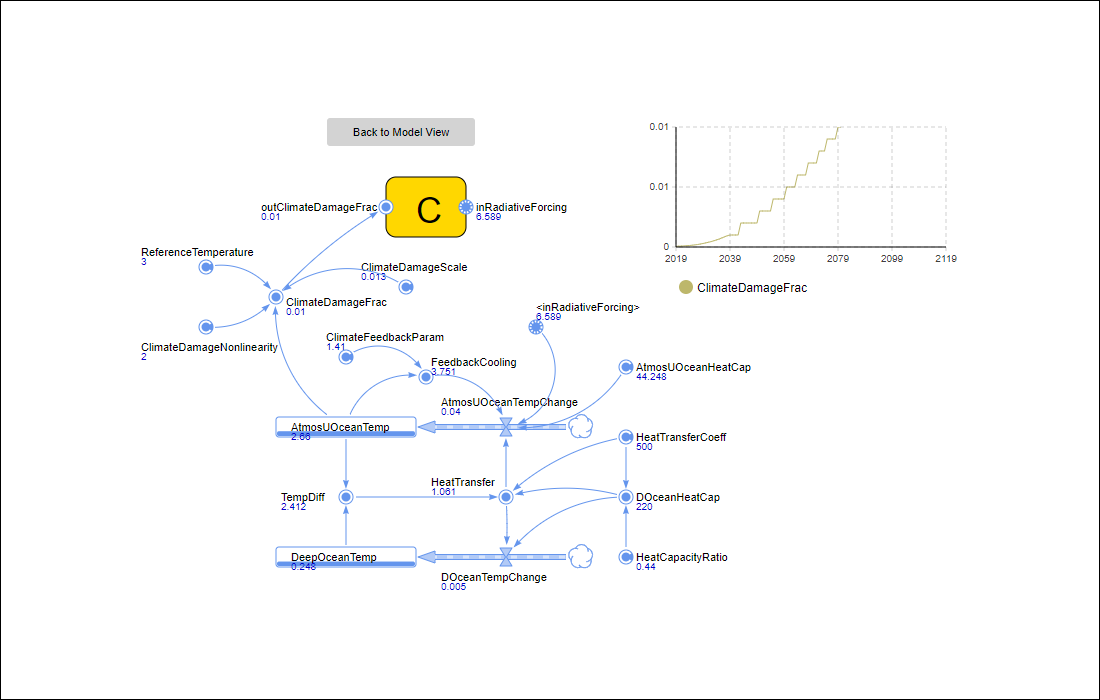
The Climate Subsystem (box B in Figure 2) takes into account the radiative forcing effects of the atmospheric CO2 and the coupled feedback loops of the heat flux between the surface and deep ocean temperature.
Mathematically, the Climate Subsystem can be captured with the following set of equations:
- Feedback Cooling = Atmos. Upper Ocean Temp. x Climate Feedback Parameter
- ΔAtmospheric Upper Ocean Temperature = (Radiative Forcing − Feedback Cooling − Heat Transfer) / Atmospheric Upper Ocean Heat Capacity
- Deep Ocean Heat Capacity = Heat Capacity Ratio x Heat Transfer Coefficient
- Heat Transfer = (Temperature Difference x Deep Ocean Heat Capacity) / Heat Transfer Coefficient
- ΔDeep Ocean Temperature = Heat Transfer / Deep Ocean Heat Capacity
- Climate Damage Fraction = 1 + Climate Damage Scale (1 / ((Atmos. Upper Ocean Temperature / Reference Temperature)^Climate Damage Nonlinearity)
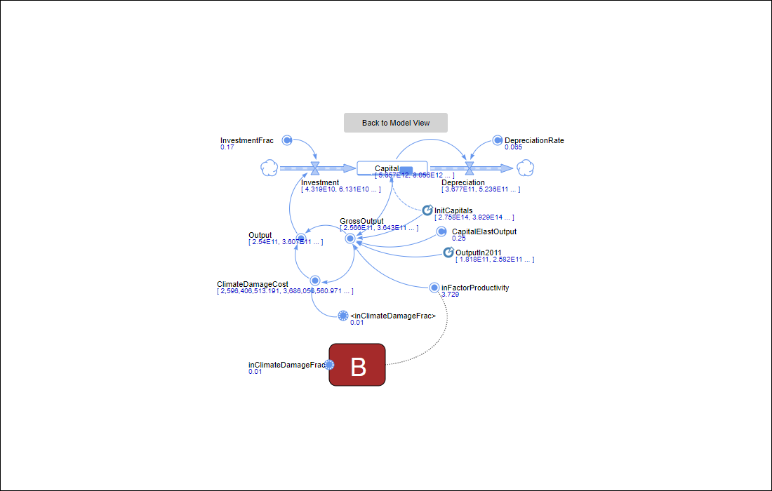
The Economy Subsystem (box C in Figure 2) consists of two feedback loops which facilitate capital accumulation through reinvestment and depreciation. The rate of output generation from capital accumulation is dictated by an exogenous input of factor productivity and the cost incurred by climate change. The economic outputs contribute to the CO2 emissions and complete the primary feedback loop of the model.
Mathematically, the Economy Subsystem can be captured with the following set of equations:
- Gross Output = Factor Productivity x Capital Elastic Output
- Climate Damage Cost = Gross Output x Climate Damage Fraction
- Output = Gross Output − Climate Damage Cost
- Investment = Output × Investment Fraction
- ΔCapital = Investment – Depreciation
The Exogenous Drivers (box D in Figure 2) reveal the second order feedback structures of two exogenous factors that have been introduced previously: CO2Intensity and FactorProductivity.
Mathematically, the Exogenous Drivers can be captured with the following set of equations:
- ΔCO2 Intensity Decline Rate = CO2 Intensity Decline Rate x Decline Rate
- ΔCO2 Intensity = CO2 Intensity x CO2 Intensity Decline Rate
- ΔFactor Productivity Growth Rate = Fact. Prod. Growth Rate x Decline Rate
- ΔFactor Productivity = Factor Productivity x Factor Productivity Growth Rate
The Fiddaman model, by default, derives the emissions from outputs in an aggregated fashion. However, the HCAM takes a different approach by outsourcing the computation to the pool of disaggregated agents (labelled E in Figure 2).
Capturing large populations through collective person agents
Simulation of agents based on raw population sizes of countries or even the entire world proves computationally extremely demanding. As a solution, the population of a model can be scaled down (e.g. to a ratio of 250,000 to 1), so that the simulation can run at an acceptable speed while still representing the entire population. This feature conveniently enables system requirements to be tailored for a wide range of computing power. The idea (inspired by Köhler et al. 2009) is to create Collective Person Agents (CPAs) that represent groups of likeminded people based on similarity in their potential behaviour. The assumptions held under such scheme are that a CPA now represents a group of people and the people within each group are homogeneous. The downside of this is the decrease in granularity and precision in the model performance. For gaining a better understanding of these high level descriptions it might help to refer to the Appendix.
Classifications of collective person agents
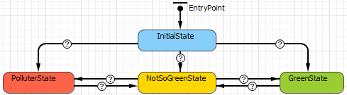
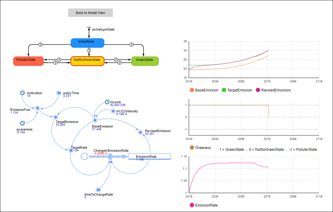
Humans can be represented collectively as CPAs. The activities of such CPAs are to consume energy, produce emissions, and network with other CPAs. They are classified into different stereotypes, based on their emission levels; these range from "green" to "polluter". The thresholds to determine the stereotypes are parameterised in order to allow the users to create multiple variations of stereotypes. Stereotypes are expressed as states in a state machine diagram (Figure 3) that is automatically created within each individual CPA. For an introduction to the topic of state machine diagrams for social simulation see Siebers & Onggo (2014). As the simulation progresses, the agents will transit into the appropriate states according to their projected emission levels and switch their representative colours to that of the new state (stereotype).
Mental model of collective person agents
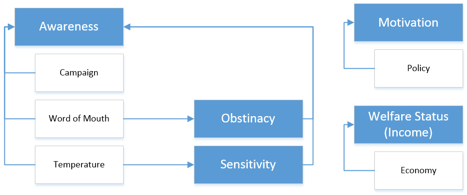
A mental model represents a CPA's knowledge about the surrounding world as well as its perception about its own actions and their consequences. Here we are using an intuitive mental model that we developed ourselves, following a very simple reflex agent architecture. It could be replaced by a more complex one (for an overview of such architectures see Balke & Gilbert 2014) in the future. A CPA possesses four mental attributes: obstinacy, awareness, motivation and sensitivity, the values of which are initially randomly assigned. The welfare status is indicated by its income. All five attributes together shape the behaviour of a CPA: the CPA's emission rate.
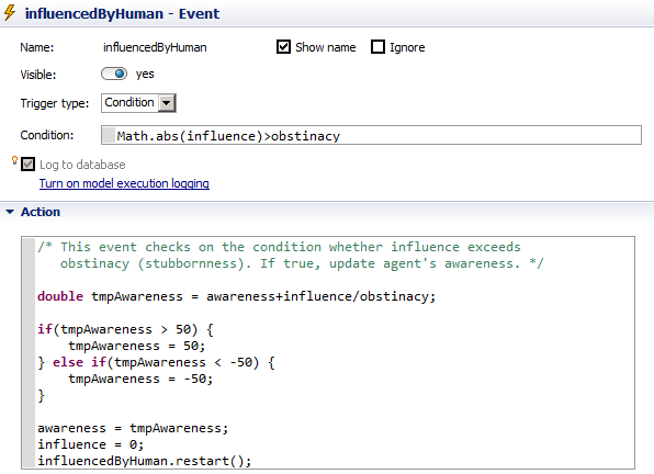
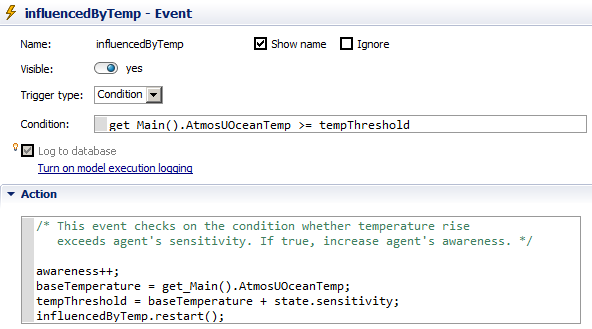
The CPAs in HCAM are subject to external influences of different sources (Figure 4). These may alter their internal attributes which are influential on their overall behaviour (motivation, awareness and income). The motivation is sourced from the implementation of external policies. It mimics the sense of obligation one undertakes in order to conform to the policy regulations. The economy takes its value from the economic output and is shared evenly among the CPAs, which forms their incomes. The awareness is subject to three types of external influences: campaigns, word-of-mouth, and temperature anomaly. These influences have to undergo certain extent of impedance before being able to make concrete changes to the awareness attribute. The effects of campaigns and word-of-mouth belong to the category of human influence, while the temperature anomaly is of a natural influence. Human influence will accumulate in an influence variable within the receiving CPA until it overcomes the obstinacy (or stubbornness) score, in order to change the CPA's awareness value. The temperature anomaly challenges the sensitivity limits of the agents. Once the temperature change exceeds the limit that one can tolerate, it increments the awareness value of the CPA.
Behaviour model of collective person agents
Producing emissions is the primary behaviour of the CPAs. It is modelled continuously in time by using an SD model inside the CPA. The SD model fragment in Figure 5 models the emission rate of each CPA by using a stock and a flow, the former being the emission rate and the latter being its rate of change. The flow of the stock is driven by the discrepancy between the BaseEmission and the TargetEmission as perceived by the CPA. The EmissionFraction is proportional to the sum of the agent's awareness and motivation indices. The motivation considers if a policy is applied or not. A RevisedEmission value is then passed to the state machine of a CPA (Figure 3). If the value is above or below a certain threshold, the stereotype (expressed as a state) of the concerning CPA will change.
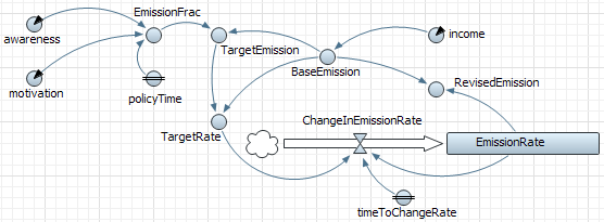
Mathematically, the emission dynamics can be captured with the following set of equations:
- Base Emission = Income × CO2 Intensity
- Emission Fraction = Awareness + Motivation(PolicyActiveOrNot)
- Target Emission = Base Emission × Emission Fraction
- Target Rate = Target Emission / Base Emission
- ΔEmission Rate = (Target Rate −Emission Rate) / Time to Change Rate
- Revised Emission = Base Emission × Emission Rate
Multi-level modelling of social structures
The social structure of the human population in HCAM is partitioned into social units of ascending aggregation levels. Social units have some kind of goal related to climate-change policies at their administrative level and can be classified under a nested hierarchy ordered by their aggregation levels: CPA ⊂ State ⊂ Region ⊂ Nation. Deducing from the formula, the unit from each level is encompassed by its parent unit, all the way to the outermost parent. Nations can be divided into clusters of regions, whereby each region embodies a set of adjacent states, and each state contains a population of CPAs. In the HCAM we use a hierarchical AB approach for representing each of the social units, i.e. each social unit is represented by an individual agent. For gaining a better understanding of these high level descriptions it might help to refer to the Appendix .
Networking
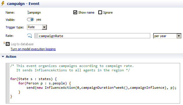
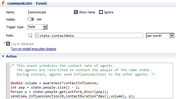
As a CPA communicates with another CPA, it is transmitting a certain amount of "influence" to the receiving CPA, which might alter the way the receiving CPA behaves in regards to emissions. All CPAs are equipped with networking modules, enabling them to communicate with each other by passing time-stamped InfluenceAction objects to each other. Such an InfluenceAction object simply consists of three variables: start, duration, and volume. While start and duration define the start and duration of the influence, volume defines the strength of it. This communication is equivalent to what is commonly known as spreading the word-of-mouth. CPAs are restricted to only communicate with the other CPAs that are in the same state. The objective of a communication process is to influence the engaged CPAs, either positively or negatively. Intuitively, a CPA with a positive awareness index will spread a positive influence and the opposite goes for a CPA with a negative awareness index. The influence cycle is guarded by two dynamic events, one for launching an influence action and another for terminating it. When the cycle terminates, a portion of the influence remains as memory while the rest is deducted from the agent's "influence" variable. Influences can also be controlled during simulation runtime by an authority (nation; region; state) in form of campaigns. A campaign influences the "strength" of the message passed between CPAs during communications. For gaining a better understanding of these high level descriptions it might help to refer to the Appendix.
Policies
There are two different policies we consider: Carbon Reduction Policy and Awareness Campaign Policy. A Carbon Reduction Policy induces motivation on CPAs to cut down on their emissions. As the enforcement of policy is often obligate and oppressive, the motivation that it creates generally reflects more of a fear factor of exceeding the carbon quota rather than a genuine commitment from the public. Nonetheless, it is effective as it can drive the carbon intensity down in a short period of time. This policy can be implemented at national or regional level. An Awareness Campaign Policy seeks to solve the problem from a different angle, by tackling the root cause of the problem. As uncontrolled carbon emissions are due to ignorance of the public, the organisation of campaigns aims to raise public awareness on environmental issues, which in the long run would cultivate more sustainable lifestyles among the public. It works by fundamentally altering the mental states of people (or CPAs in our case), which causes them to reduce their emissions. This campaign can be implemented at national or regional level. The "Spreading the Word-of-Mouth" activity is related to the information exchange resulting from the interactions between CPAs. This information exchange aims to spread environmental awareness among the public and eventually changing the behaviours of the CPAs in producing emissions. Influences received by the CPAs can be positive or negative depending on the nature of the sender. Also, the CPAs all have varying levels of resistance against the word-of-mouth influences. Therefore, some CPAs may be easily persuaded to decrease (or increase) their emissions while for some this may not be as easy. For gaining a better understanding of these high level descriptions it might help to refer to the Appendix.
Output
The outputs coming from such a HCAM are multifaceted and in the form of dynamic observables (measurable characteristics of interest) at system and individual level and statistics. They differ from those provided by traditional IAMs (i.e. steady state optimisation models) in that they provide insights at different levels of granularity. Their primary role is not to drive the model's dynamics, but to help understand the dynamics inherent in the system under study.
Throughout the runtime of a simulation we have access to all stocks and flow values inside the SD layer of our HCAM and can create time series outputs related to the dynamics of the economic and climate system over time. As we have a social structure represented by a hierarchical AB model, we can also collect information about the impact of policies on specific geographical units (e.g. regions or states). As in AB models the evolution of system-level observables does emerge from the interactions of the individual elements within the model, we will be able to observe phenomena and pattern at system level that have properties that are decoupled from the properties of the elements contributing to it.
The representation of CPAs allows us to collect behavioural related information, e.g. when someone of a specific character type would change its opinion, and how that timing differs from someone with a different character type. But we can also analyse more theoretical (e.g. through extreme case simulation experiments) how CPAs evolve over time when they start with the same settings, but are under different influences (e.g. due to different regulations and campaigns in different states). There are many more opportunities the AB layer offers to the modeller. Again, we would also expect to be able to see some emergence of phenomena and patterns at system level.
This multitude of simulation outputs allows us to gain deeper insight into the causes of climate change, dependencies, and the impact of different policies.
An Illustrative Example
The main purpose of this illustrative example is to demonstrate how to use the novel features of the HCAM described above. It shows how such a model could provide more insight and stimulate debate, through a more granular control of the system and a more granular level of outputs (from national to CPA level). The results of experiments with the current implementation are useful for relative comparisons (as all scenario outputs are based on a model with the same assumptions) and therefore to support understanding. Its purpose is not to produce meaningful results for policy advice. For that purpose, it would need to be extended, by lifting some of the assumptions (e.g. implementing a population growth model). We want to encourage researchers to use the illustrative example as a playground to test out their own ideas. The simulation model is implemented in AnyLogic and is available at https://www.comses.net (see Section 7 for details). Our test case takes the settings of the US, as this country contributes to the majority of the global carbon footprints and is the largest economic power in the world. This creates a good opportunity to investigate the carbon emissions and its relevant economic impacts on the nation. We consider the US as a whole, as well as on a state and regional basis and look at the following question: "Given a constant amount of capital allocated for climate mitigation sector, what is/are the most effective policy(s) that the federal government can invest the funds in to leverage the available resources?".
Model Design
The design of our model is using the base model presented in Section 3.6 as a starting point. In order to be able to represent a regional disaggregation of the Economy Subsystem [box C in Figure 2] for the US we used the idea of a multi-layered SD model, as presented in Kim & Juhn (1997). This method allows using SD as a modelling platform for multi-agent systems. In our case we use it to represent US regions and states.
The global CO2 emissions are the sum of emissions from the US and those from the rest of the world. As the model simulates policy analysis of the US emissions control, non-US emissions are set to change in proportion to changes in US levels, while the carbon abatement policy is designated as an exogenous input. Other exogenous variables include the factor productivity growth rate (which represents change in the level of technological sophistication that drives the economy) and CO2 intensity (which determines the emission levels of individuals based on their income). The source of the population factor takes the inputs from a population of human agents in the AB model. The assumptions that the model holds are (1) that the factor productivity increases exponentially, which causes the economic output to increase exponentially as well, (2) that the population size remains constant, without any birth or death rate, (3) that CPAs are able to adjust their emissions without direct economic impact should they be inclined to do so, and (4) that all nations other than the US are treated as following US trends in carbon output, moving proportionally to changes in US emissions rates. All of these assumptions simply the models but can be removed by modular addition of models. For example, a system dynamics model could be used to model population growth without effecting the running model. Similarly, exogenous emissions can be modelled as growing at a first or second order rate, or even generated with an additional HCAM model parameterised for other countries and run in parallel. The advantage of a modular design allows for these subcomponent extensions where important.
Data sources
The data we used for the model come from multiple sources. The information of EPA (Environmental Protection Agency) regions individual states belong to come from the EPA website (EPA 2018). The population data for individual states come from the US Census Data website (Census 2018). The GDP (Gross Domestic Profit) data for individual states come from the Bureau of Economic Analysis website (BEA 2018) and the Net Capital Stock data for individual states come from Yamarik (2013). As the latter is only available for 2007, we decided to use 2007 as the base year for all data. Other data we used is either taken from the DICE model (Nordhaus 1992) or derived from consultation of colleagues working in the relevant fields.
Model implementation
For the implementation of our model, we used AnyLogic 7.12, and later we updated the implementation to run in AnyLogic 8.5 (AnyLogic 2019). AnyLogic is a commercial multi-paradigm simulation IDE that supports using different simulation modelling paradigms in one model. It allows combining SD model components with AB model components and vice versa (making this a hybrid modelling tool). AnyLogic is (relatively) easy to use, yet not restrictive as it includes a high-level graphical modelling language and also allows users to extend the model with custom low-level Java code. Another of its features is that it allows creating multi-layered SD models, which has been used in our case for implementing a regional disaggregation of the Economy Subsystem. Alike other SD tools, AnyLogic supports arrays for representing elements within SD models and collecting statistics. This is useful for defining a set of subsystems with the same model structure (in our case the US states) but different numerical parameters (in our case the population data for the different states, e.g. name; population size). Arrays allow creating a single diagram for all the layers. Therefore, the model remains compact, and changes one makes when implementing the model will affect the whole model, not just a single layer. Details about the implementation of the dynamics inherent in the behaviour change models presented in Section 3.16 to 3.24 can be found in the Appendix. The screenshots there provide an overview of all relevant functions and events within the behavioural change models.
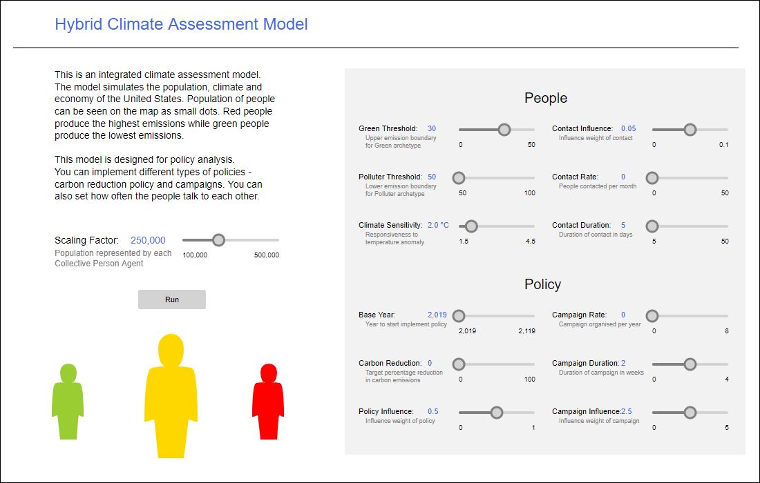
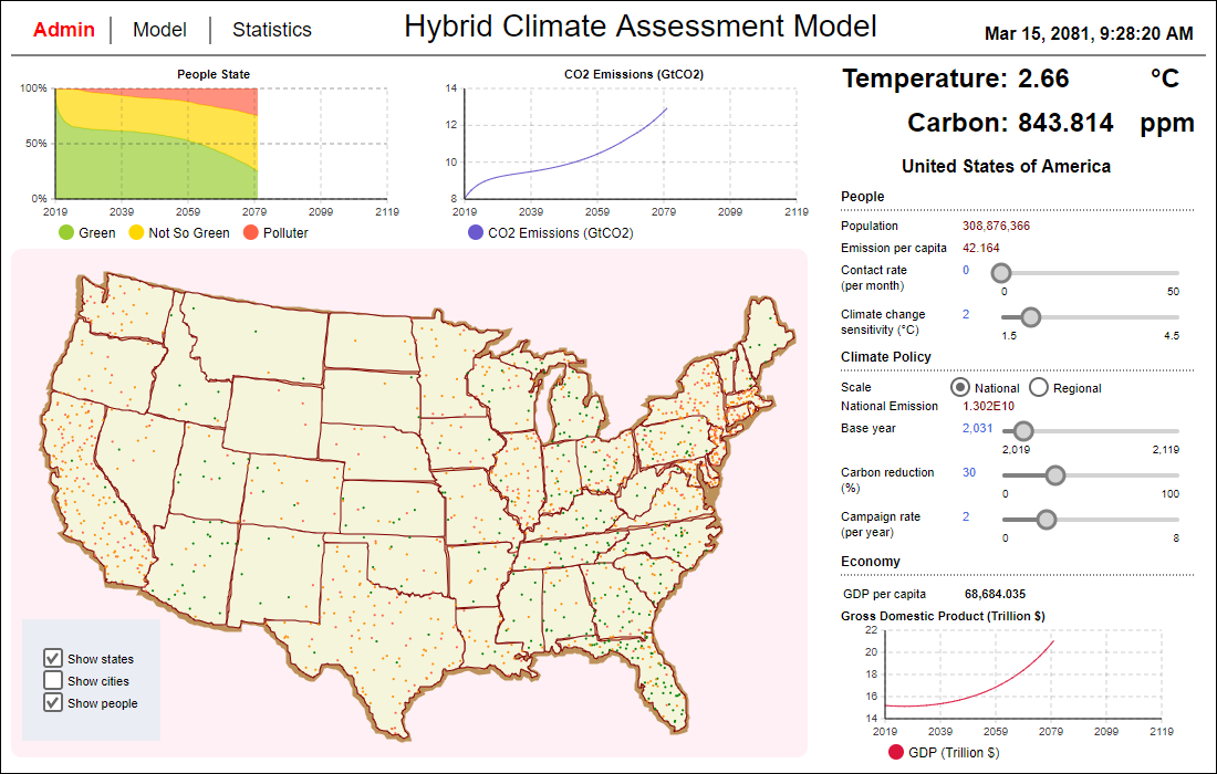
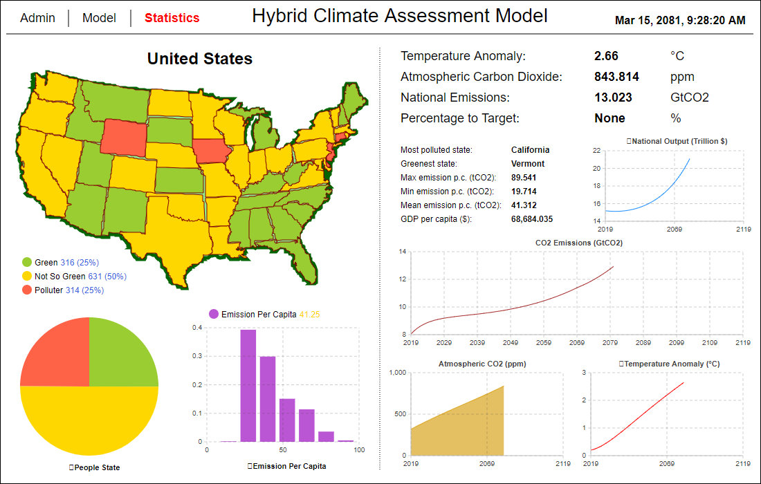
The model has been implemented as a visual interactive simulation. This means that it produces a dynamic display of the system model, and allows the user to interact with the running simulation (O'Keefe 1987). In our case the simulation model has a setup screen to define the scenario (Figure 6) and some opportunities to manipulate initial scenario settings during runtime to imitate policy implementations (Figure 7). It also produces visualisations of output data (state of the system and stats) during runtime (Figure 8-13).
Model validation and calibration
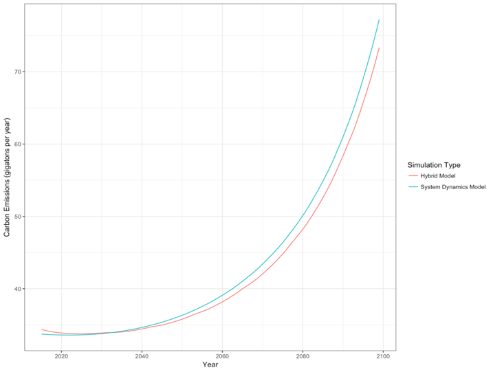
We implemented two model versions for our illustrative example: a simplified version of the original Fiddaman model (using SD modelling only) and a HCAM (using SD and AB modelling jointly), both tuned for the question to be investigated. We validated the output of the simplified version against the original DICE results (as published in Nordhaus 1992) and then calibrated the HCAM against the simplified version, to create a base case in which both behave the same (considering practical rather than statistical significance). For the comparison we used time plots of the following key indicators: CO2 Emissions, Atmospheric CO2, Temperature Anomaly, and Climate Impact on Economy. We ended up with a conformance sufficient for our purposes. Figure 14 shows a comparison of the Emissions observed in the outputs of the two with the national government attempting a carbon reduction policy of 40%.
Experimentation
As stated in Section 3.24 , there are two general policies we can consider: carbon reduction policy and awareness campaign policy. We defined four scenarios to be tested: Baseline (BL): "as-is" scenario that assumes no mitigation actions to be taken, Balanced (BA): assumes evenly-split spending on carbon reduction and campaigning, in which the carbon reduction target of 17% (per 5 years) is based on the target set by the previous US President Obama in 2015 for 2020, Extreme Campaign (EC): all funding is spent on organising campaigns, and Extreme Reduction (ER): all funding is invested in carbon abatement. A summary of scenarios can be found in Table 1. For population scaling we used a ratio of 250,000 to 1 during the experiments.
| Policy | ||
| Scenario | Carbon reduction (%) | Campaigns (per year) |
| Baseline (BL) | 0 | 0 |
| Balanced (BA) | 17 | 4 |
| Extreme Campaign (EC) | 0 | 8 |
| Extreme Reduction (ER) | 34 | 0 |
To compare the impact of applying the different policies, we collected the following simulation outputs as key indicators: CO2 Emissions, Atmospheric CO2, Temperature Anomaly, and Climate Impact on Economy. We collected the data in form of time plots for 80 years (from 2015 till 2095). The results of the experiment are presented in Figure 15.
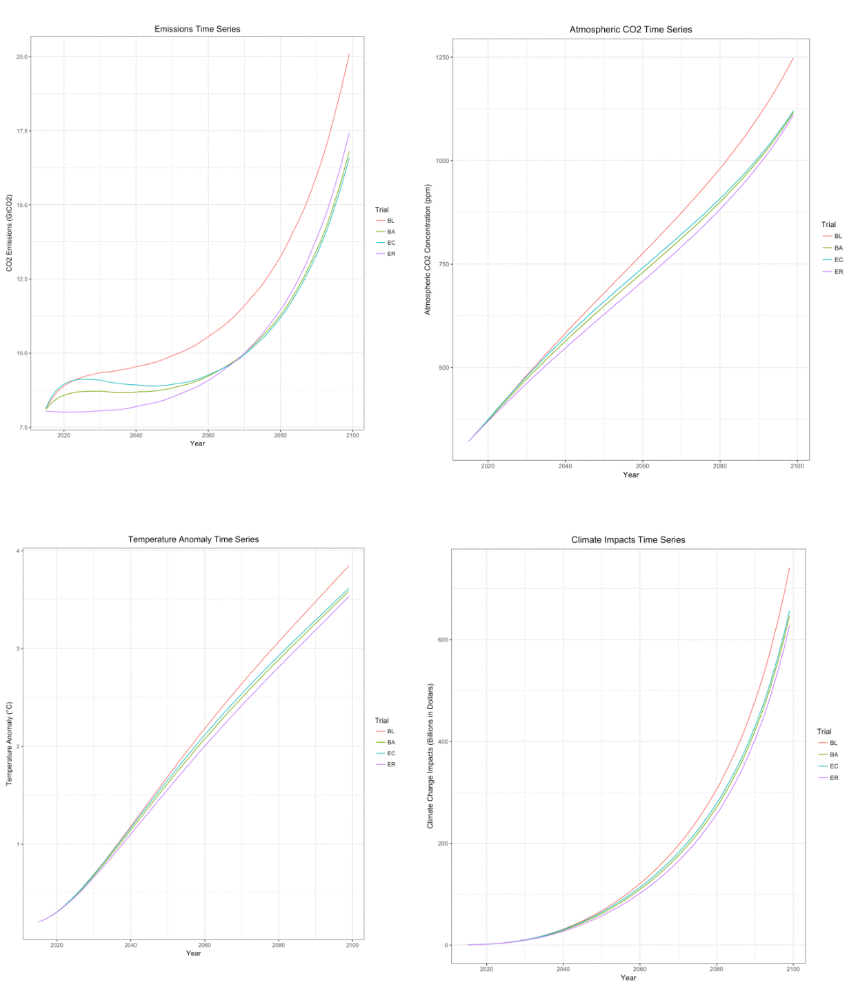
According to the CO2 Emission, time series EC emerges as the best-performing scenario, with a more balanced and toned-down policy approach. It is, however, only slightly better than BA, with a difference of 0.2 GtCO2 in their final emissions. As for the rest of the indicators, atmospheric CO2, temperature anomaly and climate damage, there is not much interesting information to deduce from them, although ER outperformed the other interventions, likely due to the more immediate emissions reductions compared with campaign based interventions. The resulting trends of the scenarios are as expected, that atmospheric CO2 concentration and temperature anomaly of each scenario are generally correlated with their corresponding compounded emissions level. Besides, the differences between scenarios are relatively slight, likely due to the relatively reserved nature of these interventions. When considering the global results, specifically temperature anomaly and atmospheric CO2 levels, it is worth remembering the built in assumption that non-US emissions vary proportionally to US levels. In practice this assumes that other countries perform similar interventions through a mechanism such as international climate agreements.
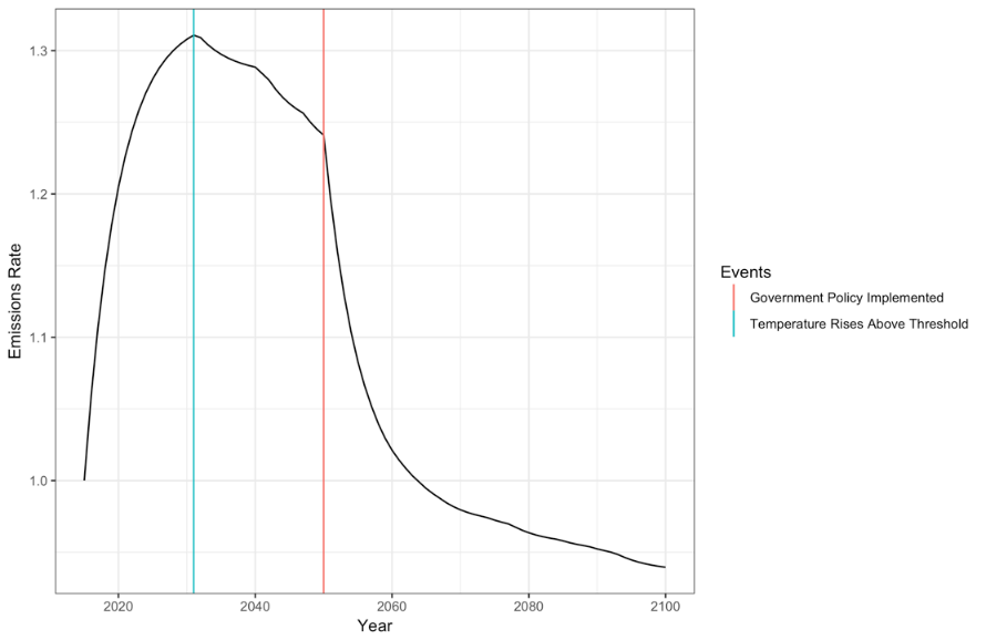
As we model the population (in form of CPAs with specific stereotypes) and the social structures (states and regions) using an agent-based approach we can gain additional lower level insight. Figure 16 shows the changes within an individual CPA during a simulation run. The temperature threshold for that agent, whereupon they became aware of the effect of emissions on the climate, occurred in 2031 of the simulation model. In this run, the government was scheduled to instigate an aggressive carbon reduction policy in the year 2050, attempting to reduce emissions 10% below the initial base year. This allows analysis of behaviour at an individual level with asymmetric stereotypes.
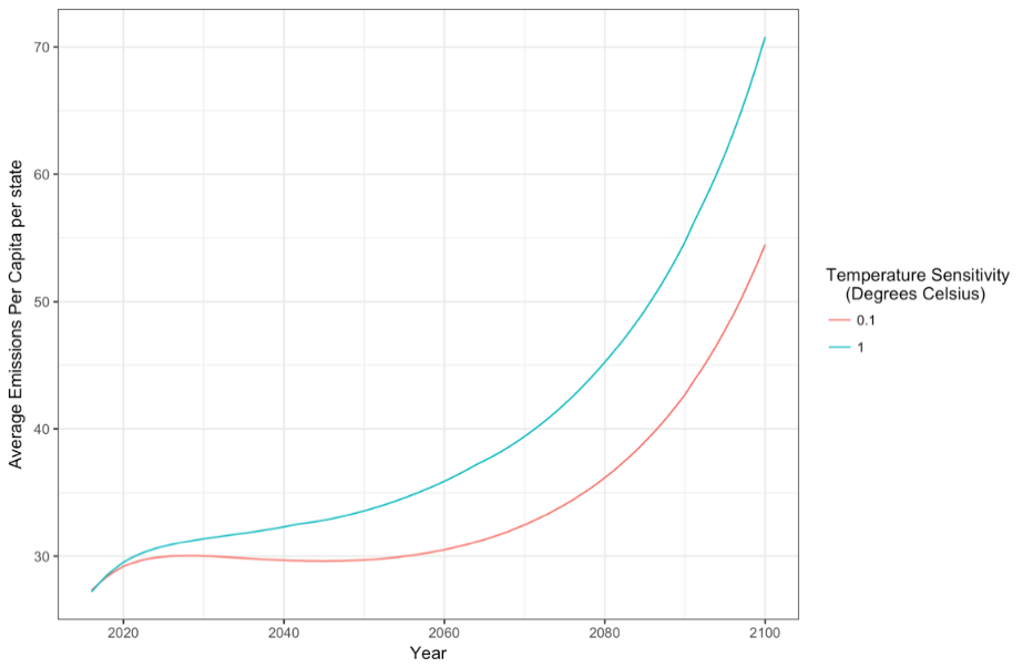
A use case for the agent hierarchy in this model could be that populations of different states may have different sensitivities to changes in climate. For example, states with a large amount of tourism and agriculture may be much more sensitive to temperature changes than other states. This is demonstrated in Figure 17, where states were randomly assigned a "sensitive to temperature changes" value of either 0.1 °C (sensitive) or 1 °C (insensitive). It can be seen that in the model agents in sensitive states reduce emissions earlier and to a greater degree when compared with insensitive states. Parametrising this "sensitive to temperature changes" value using methods such as survey data would therefore allow for granular analysis of emissions on a state or regional level.
Conclusions and Further Work
In this paper we have introduced a hybrid climate assessment modelling concept called HCAM and we have demonstrated its application by providing an illustrative example. The HCAM concept allows to reuse components of existing rigid, but well-established IAMs, and adding more flexibility through replacing aggregate stocks with a scalable community of vibrant interacting entities. Furthermore, by combining top-down SD modelling and bottom-up AB modelling approaches, we can create IAMs that allow studying the disequilibrium dynamics of the system over time. Our illustrative example for demonstrating the application of HCAM focused on providing some insight into carbon emission dynamics of individual states within the US and its relevant economic impacts on the nation over time. By using CPAs for representing large groups of like-minded people we were able to use an AB modelling approach to represent the whole of the US population, and still run the simulation on a normal PC in a reasonable amount of time.
Applying a hybrid modelling approach and multi-level modelling allowed us to not only look at system level outputs, but to study local differences and analyse the influences of political decisions at different levels of abstractions. We could, for example, look at individuals and groups and see if political changes have stronger or weaker influences at specific groups of people (which share the same stereotype) and if these influences change over time. All of this helps us to better understand the dynamics of the system and its components over time and adds transparency. Further benefits are the ability to interact with the model during runtime (e.g. by adding ad-hoc interventions and observing their effect over time) and to get away from a steady state to a dynamic model that allows capturing non equilibrium scenarios. Our HCAM considers a lot of (behavioural and mental) details within the agents which is often missing in other AB models. Also, the interactive environment invite to explore the solution space by providing interactive components whose settings can be changed during runtime and outputs at different levels of granularity. Due to its GUI and real-time output presentation it also stimulates group communication as the simulation can be run as part of a team exercise.
Regarding limitations, one should be aware that we are providing a proof-of-concept illustrative example here that is based on a long list of assumptions and simplifications (for more details see Section 4.1). In addition, the behavioural models embedded in the agents are somewhat simplistic. However, having a modular object oriented design allows for replacing relevant sub-systems once more sophisticated behavioural models are found.
There are many possibilities to move forward from here. So far we have deliberately tried to keep it simple and to focus on demonstrating a methodological advance (i.e. how to use the conceptual ideas of the HCAM in practice). From a modelling point of view, the CPA decision making would definitely benefit from being improved. Currently emissions are processed inside the CPA using a SD model instead of using more realistic discrete decision making events. Therefore, it is difficult to introduce reasoning and intelligence to the emission decision making. An alternative approach would be to borrow from Artificial Intelligence community and to use a Belief-Desire-Intention (BDI) approach for the decision making process. The integration of a BDI approach within HCAM would enhance the current agent model with more realistic behaviours, driven by their beliefs (awareness, income, energy price, climate, etc.), desires (to be in green or polluter state) and intentions (consume or conserve). This could also be extended to social structure agents. From a computational point of view it would be interesting to work out what the impact of the scaling is (i.e. using CPAs) and how far we could go with this approach.
Overall, we hope that we have provided some stimulation for others to consider this hybrid approach to integrated assessment modelling in the future and that we will see some real world applications of our HCAM concept in the near future.
Model Documentation
The HCAM model was updated and tested to run in AnyLogic PLE 8.5 and the code is available at: https://www.comses.net/codebases/e0c890e9-599f-4539-ad48-f59130083b31/releases/1.0.0/.Appendix
Below we provide some more details about the dynamics inherent in the behaviour change models presented in Section 3.16 to Section 3.24. Table 2 provides an overview of all relevant parameters to be set before the actual simulation starts. These will then be used in the code snippets provided in the following screenshots. The screenshots provide an overview over all relevant functions and events within the behavioural change models in a hierarchical order: From Nation to CPA.
- Before execution the following relevant parameters are set:
| Parameters | Explanation |
| Sensitivity | Responsiveness to temperature anomaly |
| CarbonReduction | Target percentage reduction in carbon emission |
| CampaignRate | Campaigns organised per year |
| CampaignDuration | Duration of campaign in weeks |
| BaseYear | Year to start implement policy |
| CampaignInfluence | Influence weight of campaign |
| GreenThreshold | Upper emission boundary for Green archetipe |
| PolluterThreshold | Upper emission boundary for Polluter archetipe |
| PolicyInfluence | Influence weight of policy |
| ContactRate | People contacted per month |
| ContactDuration | Duration of contact in days |
| ContactInfluence | Influence weight of contact |
- At national level
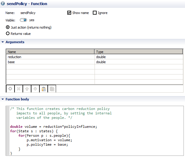
- Carbon policy setup is defined for all regions during simulation start up
- Parameters used: sendPolicy(carbonReduction,baseYear)
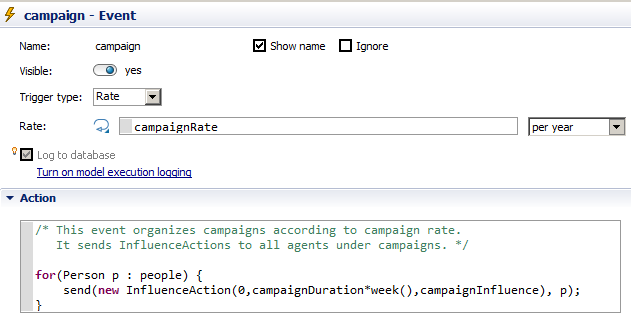
- Campaigns are organised for all regions at a certain rate
- Carbon policy setup is defined for all regions during simulation start up
- At regional level
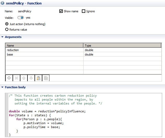
- Carbon policy setup for region is altered during runtime when slider is moved
- Parameters used: sendPolicy(carbonReduction,baseYear)
- An InfluenceAction object is send to all states within a region at irregular intervals (campaignRate times per year) to update their campaignInfluence variable (i.e. the intensity of influences)
- InfluenceAction is an object that just consists of three parameters: start, duration, volume; the parameter volume refers to the intensity of the influence
- Carbon policy setup for region is altered during runtime when slider is moved
- At CPA level
- Awareness is updated as a result of word-of-mouth communications when influence through communication is high enough to overcome stubbornness
- Awareness is increased when temperature rise in atmosphere and ocean has exceeded CPA's sensitivity limits
- An InfluenceAction object is send to a random CPA within a state at irregular intervals (state.ContactRate times per year) to update their volume variable (i.e. the intensity of influences)
References
ANYLOGIC. (2019). AnyLogic. https://www.anylogic.com/.
AXELROD, R. (1997) 'Advancing the Art of Simulation in the Social Sciences.' In: Conte R, Hegselmann R, & Terna R (eds.) Simulating Social Phenomena. Springer: Berlin, Germany.
BALKE, T. & Gilbert, N. (2014). How do agents make decisions - A survey. Journal of Artificial Societies and Social Simulation, 17(4)13. https://www.jasss.org/17/4/13.html. [doi:10.18564/jasss.2687]
BEA. (2018). Bureau of Economic Analysis. https://www.bea.gov/.
BONABEAU, E. (2002). Agent-based modeling: Methods and techniques for simulating human systems. Proceedings of the National Academy of Sciences, 99(suppl 3), 7280-7287. [doi:10.1073/pnas.082080899]
BORSHCHEV, A. (2013). The Big Book of Simulation Modeling: Multimethod Modeling with AnyLogic 6. North America: AnyLogic.
BOX, G. E. (1979). Robustness in the strategy of scientific model building. In: R. L. Launer & G. N. Wilkinson (Eds.), Robustness in Statistics. Academic Press. [doi:10.1016/b978-0-12-438150-6.50018-2]
CARBONBRIEF. (2018). CarbonBrief: Clear on Climate. https://www.carbonbrief.org/analysis-how-much-carbon-budget-is-left-to-limit-global-warming-to-1-5c.
CENSUS. (2018). United States Census Bureau: Population Estimates. https://www.census.gov/data/tables/time-series/demo/popest/2010s-total-metro-and-micro-statistical-areas.html
CHOOPOJCHAROEN, T. & Magzari, A. (2012). Mathematics behind System Dynamics. BSc Dissertation: Worcester Polytechnic Institute, UK.
CLIMATE INTERACTIVE. (2016). C-ROADS: Climate Change Policy Simulator. https://www.climateinteractive.org/tools/c-roads/.
COUCLELIS, H. (2002). Modeling frameworks, paradigms, and approaches. In K. C. Clarke, B. O. Parks , & M. P. Crane (Eds.), Geographic Information Systems and Environmental Modelling, London, UK: Prentice Hall.
CRAIG, A. N. & Burns, W. C. G. (2016). Climate Engineering under the Paris Agreement: A Legal and Policy Primer. Technical Report.
EPA. (2018). United States Environmental Protection Agency: Regional Offices. https://www.epa.gov/aboutepa#pane-4.
FIDDAMAN, T. S. (1997). Feedback Complexity in Integrated Climate-Economy Models. Doctoral Dissertation: Massachusetts Institute of Technology.
FORRESTER, J.W. (1961). Industrial Dynamics. Portland, OR: Productivity Press.
GILBERT, N. & Troitzsch, K. (2005). Simulation for the Social Scientist (2nd Edition). UK: McGraw-Hill Education.
IPCC. (2014). Climate Change 2014 Synthesis Report: Summary for Policymakers. https://www.ipcc.ch/pdf/assessment-report/ar5/syr/AR5_SYR_FINAL_SPM.pdf.
KIM, D. K. & Juhn, J. H. (1997). System dynamics as a modeling platform for multi-agent systems. IProceedings of the 15th International Conference of the System Dynamics Society, Istanbul, Turkey.
KÖHLER, J., Whitmarsh, L., Nykvist, B., Schilperoord, M., Bergman, N., & Haxeltine, A. (2009). A transition model for sustainable mobility. Ecological Economics, 68(12), 2985-2995. [doi:10.1016/j.ecolecon.2009.06.027]
KOTZ, C. & Hiessl, H. (2005). Analysis of system innovation in urban water infrastructure systems: An agent-based modelling approach. Water Science and Technology: Water Supply, 5(2), 135-144. [doi:10.2166/ws.2005.0030]
LÄTTILÄ, L., Hilletofth, P., & Lin, B. (2010). Hybrid simulation models - When, why, how? Expert Systems with Applications, 37(12), 7969-7975. [doi:10.1016/j.eswa.2010.04.039]
LEMOINE, D. & Traeger, C. (2014). Watch your step: Optimal policy in a tipping climate. American Economic Journal: Economic Policy, 6(1), 137-166. [doi:10.1257/pol.6.1.137]
METCALF, G. & Stock, J. (2015). The role of integrated assessment models in climate policy: a user's guide and assessment. Discussion Paper 2015-68. Cambridge, Mass.: Harvard Project on Climate Agreements.
MORECROFT, J. (2007). Strategic Modelling and Business Dynamics: A Feedback Systems Approach. Hoboken, NJ: John Wiley & Sons.
MOSS, R. H., Edmonds, J. A., Hibbard, K. A., Manning, M. R., Rose, S. K., Van Vuuren, D. P., Carter, T. R., Emori, S., Kainuma, M., Kram, T., & Meehl, G.A. (2010). The next generation of scenarios for climate change research and assessment. Nature, 463(7282), 747-756. [doi:10.1038/nature08823]
NORDHAUS, W. D. (1992). The 'DICE' Model: Background and Structure of a Dynamic Integrated Climate-Economy Model of the Economics of Global Warming. Cowles Foundation for Research in Economics, New Haven, CT: Yale University.
NORDHAUS, W. D. & Yang, Z. (1996). A regional dynamic general-equilibrium model of alternative climate-change strategies. The American Economic Review, 86(4), 741-765.
NORDHAUS, W. D. (2017) Scientific and Economic Background on DICE models: https://sites.google.com/site/williamdnordhaus/dice-rice.
O'KEEFE, P. M. (1987). What is visual interactive simulation? Proceedings of the 1987 Winter Simulation Conference, Atlanta, GA.
PEREZ, P., Banos, A., & Pettit, C. (2017). Agent-based modelling for urban planning - current limitations and future trends. In: M. R. Namazi Rad, L. Padgham, P., K. Nagel, & A. Bazzan (Eds.) Agent Based Modelling of Urban Systems. Springer. [doi:10.1007/978-3-319-51957-9_4]
PHELAN, S. E. (1999). a note on the correspondence between Complexity and Systems Theory. Systemic Practice and Action Research, 12(3), 237-246.
SHAFIEI, E., Stefansson, H., Asgeirsson, E. I., Davidsdottir, B., & Raberto, M. (2013). Integrated agent-based and system dynamics modelling for simulation of sustainable mobility. Transport Reviews, 33(1), 44-70. [doi:10.1080/01441647.2012.745632]
ROSHAN, E., Khabbazan, M. M., & Held, H. (2019). Cost-risk trade-off of mitigation and solar geoengineering: considering regional disparities under probabilistic climate sensitivity. Environmental and Resource Economics, 72(1), 263-279. [doi:10.1007/s10640-018-0261-9]
SIEBERS, P. O., Aickelin, U., Celia, H. & Clegg, C. (2007). A multi-agent simulation of retail management practices. Proceedings of the 2007 Summer Computer Simulation Conference, San Diego, CA. [doi:10.2139/ssrn.2831284]
SIEBERS, P. O. & Onggo, B. S. S. (2014). Graphical representation of agent-based models in operational research and management science using UML. Proceedings of the 7th OR Society Simulation Workshop (SW14), Worcestershire, UK.
UNITED NATIONS. (2015). Paris Agreement. https://unfccc.int/sites/default/files/english_paris_agreement.pdf.
VAN DYKE Parunak, H., Savit, R., & Riolo, R. L. (1998). Agent-based modeling vs. Equation-based modeling: A case study and users' guide, Proceedings of Multi-Agent Systems and Agent-Based Simulation Conference (MABS'98), 10-25, Springer, LNAI 1534. [doi:10.1007/10692956_2]
WEYANT, J. (2017). Some contributions of integrated assessment models of global climate change. Review of Environmental Economics and Policy, 11(1), 115-137. [doi:10.1093/reep/rew018]
WSC. (2015). Proceedings of the Winter Simulation Conference 2015 / Hybrid Track. http://www.wintersim.org/2015/hybrid.html.
YAMARIK, S. (2013). State‐level capital and investment: Updates and implications. Contemporary Economic Policy, 31(1), 62-72. [doi:10.1111/j.1465-7287.2011.00282.x]