
Introduction
Land use and land cover change (LULCC) has been playing a critical role in driving landscape dynamics of watershed ecosystems. These ecosystems are often coupled human and natural systems (Liu et al. 2007a; Liu et al. 2007b) in which anthropogenic activities or policies may lead to alternative consequences in terms of watershed conditions (Haidary et al. 2013). The condition of a watershed such as water quality is inherently related to land cover patterns (e.g., impervious cover, forest, and farmland) that have been modified by spatial processes of urbanization, deforestation, or agriculture activities. A set of models, represented by impervious cover model (Kauffman & Brant 2000; Schueler 1994) and forest cover model (Gerow et al. 2015, 2016), have been proposed to study the relationship between land cover and water quality at the watershed level. A threshold effect of percent land cover (e.g., impervious cover or forest cover) on water quality at the watershed level has been identified in the literature. Watersheds within this threshold are at a tipping point that may transit to other equilibriums in terms of water quality (good or poor) in response to alternative land management practices or policies. A number of empirical studies have reported this threshold effect, which may be specific to watersheds of interest (Schueler et al. 2009). For example, a range of 10-25% of percent urban cover is a generic critical threshold based on the impervious cover model (Schueler 1994). 37-48% of percent forest cover was identified as a critical threshold of water quality specific to the High Rock Lake Watershed in North Carolina, USA (Gerow et al. 2015, 2016).
Threshold effects in terms of water quality at (sub) watershed level have been well established in the literature. Most of the studies are based on the use of historic or present data (land cover and indicators of water quality) to identify those regions within the threshold (Haidary et al. 2013; Schueler et al. 2009). The identification of these potential regions in a watershed is very important for the regulation of water quality, watershed management practices, and landscape conservation. Once these regions are degraded (transition to a different equilibrium), the restoration process may be difficult (or even infeasible), time- and cost-consuming particularly for those regions that are beyond the critical threshold (e.g., densely urbanized or heavily deforested; often irreversible) (Schueler 1994). However, the identification of where and when those potential regions in a watershed may experience threshold due to, for example, future land development or alternative policy intervention poses a grand challenge. The processes of LULCC per se and the way that LUCC affect water quality in a watershed are complex, nonlinear, and uncertain. For example, a time lag effect may exhibit in terms of the impact of LULCC on watershed-level water quality (Meals et al. 2010): the impact of LULCC on water quality may not be immediately observed. It needs a period of time (depending on indicators of interest; see Meals et al. 2010) for water quality to respond to the land development or management practices. Further, the processes associated with LULCC may not be stationary over time. Complex dynamics in these processes further complicate the identification of space-time locations of those potential regions within thresholds.
To identify these potential regions experiencing water quality threshold and their response to land development and policy intervention often requires the use of land change simulation modeling. Agent-based models (ABMs) of land systems are such a spatiotemporal simulation approach for their support in the representation of complex pattern-process interactions and scenario analysis (Epstein & Axtell 1996; Grimm et al. 2005). As one of the approaches recommended for land change modeling (Council 2014), ABMs are a bottom-up simulation approach that uses agents as building blocks to represent interactions among actors (e.g., stakeholders or land owners) or with their environments. Agents make explicit decisions on their actions based on the contextual information that they perceive from their situated environments that are often spatially heterogeneous. The explicit representation of actor decision-making and actor-environment interactions in ABMs allows for the simulation of land developments that are often complex and uncertain (Parker et al. 2003). A number of agent-based land change models have been proposed and detailed review conducted over the past two decades (An et al. 2005; An et al. 2014; Groeneveld et al. 2017; Matthews et al. 2007; Ng et al. 2011; O'Sullivan et al. 2016; Parker et al. 2003), which offers insights into the development of agent-based model in this study.
Therefore, the goal of this study is to present an agent-based land change simulation model to identify the space-time locations of potential regions experiencing critical threshold of water quality in a watershed in response to land change activities. Our study area includes eight North Carolina (NC) counties that cover the lower High Rock Lake Watershed region. This study area is representative of coupled human and natural systems in which LULCC plays an important role in driving and interpreting complex ecosystem dynamics. Land-related activities such as land development and agricultural activities render the ecosystem of this region vulnerable facing a series of issues in terms of, for example, water supply and water quality. These issues may further lead to degradation in quality of life or public health concern in this study region. Thus, such an agent-based land change simulation model is needed that allows us to investigate the potential impact of land-related activities or policies on the landscape (water quality here). The agent-based modeling approach is preferred here over other simulation approaches (e.g., cellular automata or system dynamics). This is because the agent-based modeling approach provides an integrative modeling platform that can combine with other approaches as needed and, more importantly, support the explicit representation of individual-level decision-making processes of actors (e.g., preferences of land developers or owners here) and their interactions. The remainder of this article is organized in the following manner. First, we introduce the study area and data used in this study. Second, we focus on the design of the agent-based land change model. Then, we present experimental results and discussion. This article ends with conclusion of the study.
Study Area and Data
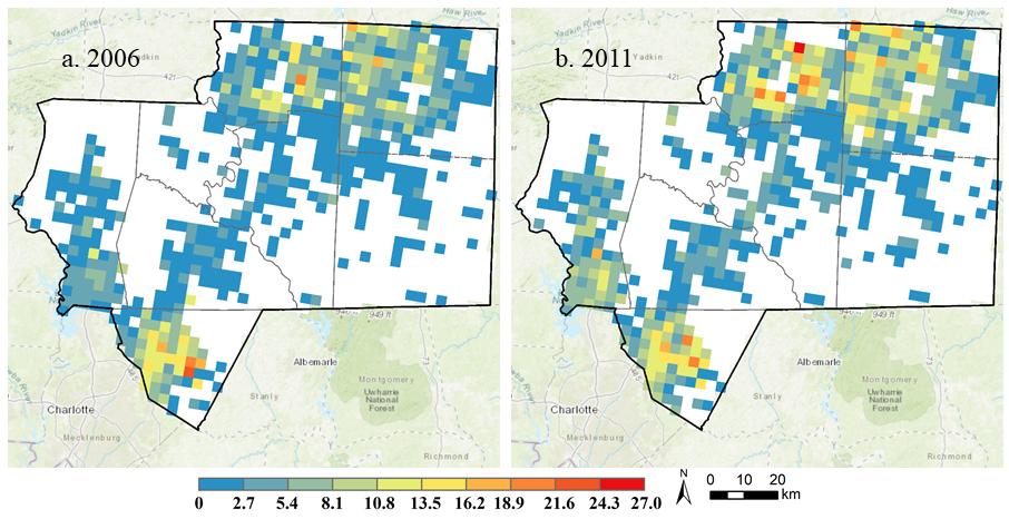
Our study region (see Figure 1) includes eight counties in North Carolina, USA, which cover the lower High Rock Lake Watershed (HRLW) area. The total area of our study region is 10,823 km2 with a total population of 1.78 million in the year of 2017. This study region is located within the Piedmont area of North Carolina, with elevation varying from 99m to 528m. Percentage of urban land cover in the study region is 18.55%, 19.56%, and 20.09% in year 2001, 2006, and 2011. This study region experienced 5.4% of increase in percent urban cover from 2001 to 2006, and this rate becomes 2.7% from 2006 to 2011 (due to the impact of economic recession).
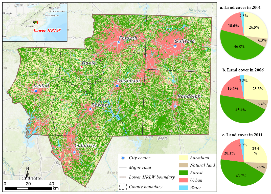
Three years (2001, 2006, and 2011) of land cover data used in this study were retrieved from U.S. National Land Cover Database (NLCD). These land cover data were available at a spatial resolution of 30m by 30m. We further aggregated these land cover data into five major types: urban (including developed areas with low, medium and high intensity, and open space), farmland (including pasture and cropland), forest (including deciduous, evergreen, and mixed forest), natural (including shrub, scrub, grassland, and barren land), and water (including open water and wetlands) (see Figure 1 and Table 1). Data of road network, cities or towns and their populations, and county boundaries were obtained from US Census website. Stream network and watershed data (12-digit Hydrologic Unit Code was used) was from the USDA National Hydrography Dataset. Elevation data is from NASA SRTM data. All the vector GIS data were rasterized using a 30m×30 spatial resolution. The landscape size is 4,378×4,746 in terms of number of rows and columns of the raster GIS data.
| Land cover | Year | Davie | Forsyth | Davidson | Cabarrus | Randolph | Rowan | Guilford | Iredell | Lower HRLW |
| Farmland | 2001 | 239.16 | 171.94 | 354.75 | 231.57 | 528.08 | 424.70 | 421.67 | 536.47 | 2908.36 |
| 2006 | 229.64 | 159.88 | 337.37 | 212.63 | 524.12 | 408.30 | 403.10 | 516.38 | 2791.43 | |
| 2011 | 228.23 | 154.88 | 335.26 | 208.72 | 517.00 | 405.92 | 394.90 | 508.46 | 2753.38 | |
| Natural | 2001 | 49.20 | 54.83 | 115.80 | 68.12 | 139.36 | 100.63 | 57.93 | 93.56 | 679.43 |
| 2006 | 48.27 | 56.86 | 112.29 | 68.36 | 148.44 | 101.42 | 62.31 | 97.41 | 695.36 | |
| 2011 | 54.22 | 66.43 | 140.65 | 78.02 | 209.40 | 118.24 | 77.89 | 111.46 | 856.32 | |
| Forest | 2001 | 326.94 | 435.07 | 748.78 | 425.74 | 1149.07 | 609.31 | 649.14 | 633.34 | 4977.39 |
| 2006 | 326.93 | 427.41 | 749.90 | 408.80 | 1138.89 | 606.02 | 631.98 | 628.83 | 4918.78 | |
| 2011 | 322.05 | 412.92 | 719.85 | 396.68 | 1071.52 | 588.92 | 604.69 | 611.57 | 4728.21 | |
| Urban | 2001 | 63.57 | 389.36 | 206.93 | 200.32 | 206.33 | 183.18 | 530.91 | 227.11 | 2007.72 |
| 2006 | 65.89 | 405.33 | 215.85 | 226.03 | 211.21 | 188.47 | 562.19 | 241.85 | 2116.81 | |
| 2011 | 66.34 | 415.31 | 219.67 | 232.63 | 215.19 | 191.27 | 580.14 | 253.74 | 2174.29 | |
| Water | 2001 | 12.91 | 17.62 | 42.49 | 18.10 | 21.51 | 38.72 | 43.51 | 55.48 | 250.33 |
| 2006 | 21.05 | 19.34 | 53.34 | 28.03 | 21.70 | 52.32 | 43.60 | 61.49 | 300.86 | |
| 2011 | 20.94 | 19.28 | 53.32 | 27.79 | 31.25 | 52.18 | 45.55 | 60.73 | 311.04 |
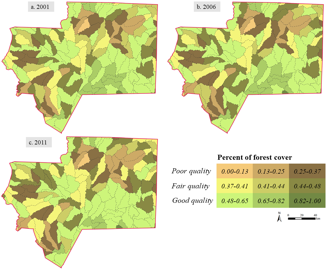
The High Rock Lake in our study region have been facing a water quality issue due to the nutrient loads from, for example, land use and management activities. This water quality issue in this region has received considerable attention from government agencies such as US Environmental Protection Agency and NC Forest Service. NC Forest Service developed a forest cover model to evaluate the relationship between forest cover and water quality in the HRLW region (Gerow et al. 2015, 2016);. Benthic macroinvertebrates are aquatic organisms (most of them are aquatic insects) that are sensitive to the conditions of their living environments, and have been extensively used as indicators of water or habitat quality (Mandaville 2002). A series of metrics based on structural or functional characteristics of benthic macroinvertebrate communities have been developed to evaluate water conditions (Barbour et al. 1999). Based on the empirical analysis of five years of land cover data and benthic macroinvertebrate data, a range of 37-48% of percent forest cover was identified as the threshold of water quality for the HRLW region (Gerow et al. 2015, 2016). Sub watersheds (or catchments) with percent forest cover higher than 48% (or lower than 37%) correspond to good (or poor) water quality indicated by benthic macroinvertebrate metrics. Any sub watersheds with the percentage of forest cover within this range are at the tipping point with fair water quality that may be shifted to either good or poor states. Our overall study region is at this tipping point (fair water quality) as its percent forest cover varies from 45.99% down to 43.69% from 2001 to 2011. Figure 2 shows the maps of sub watershed-level water quality based on forest cover model for 2001, 2006, and 2011. Of more interest is to identify where those regions at sub watershed level are at the tipping point particularly in the future and how the conditions of these sub watershed regions may change in response to LULCC. This drives the development of the agent-based land change model in this study.
Methods
Design of the agent-based model
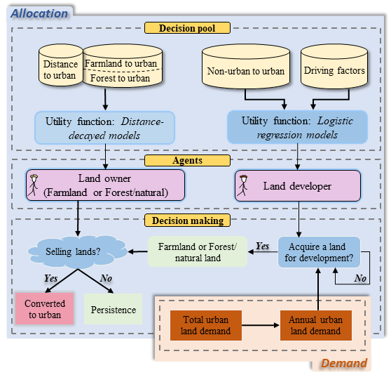
Figure 3 illustrates the architecture of the agent-based land change model in this study. The agent-based model was designed using the demand-allocation framework, which is commonly used in the land change modeling domain (Aquilue et al. 2017; Liu et al. 2017; Verburg et al. 2002). The demand-allocation land change framework consist of two modules: demand and allocation. The demand module controls the quantity of land development activities in a top-down manner and the allocation module determines where these activities will occur. The demand module can be linked to, for example, system dynamics model (Lauf et al. 2012; Liu et al. 2017) or a population density approach (McGarigal et al. 2018; Meentemeyer et al. 2013) to estimate land change demand. In this study, the land change demand in each county each year is the area of land that will be converted.
The allocation module that determines where land development will occur is driven by the interactions of two types of agents (Mustafa et al. 2017): land owners and land developers. Land owners and land developers are situated within each county. These agents interact with each other on the transactions of lands for development. Land owners decide whether to sell their lands to developers for residential development. Land developers are in charge of decision making in terms of where a residential development event will occur, the area of the development, and how to realize the development. Both land owners and land developers are hypothetical agents (Matthews et al. 2007; Valbuena et al. 2009). Through interactions between land owners and land developers, the land change allocation process is implemented in a bottom-up manner.
We documented this ABM using ODD protocol (Grimm et al. 2010) in Supplementary Material A. Please refer to the ODD protocol of the ABM for more detail. In this article, we focus on discussing the two types of agents: land owners and land developers.
Land owner agents
Land owners are in charge of management of their lands including farmlands, forest, and natural. Land owners make decisions on whether to sell their lands to developers or not (i.e., two actions). This decision is driven by land owner’s perception on surrounding environments. We used a distance-decayed model to represent land owner’s decision on selling their lands for development—i.e., the utility function of land owner agents (Lauf et al. 2012; McGarigal et al. 2018; Tang & Jia 2014). Land owner’s decision on selling their lands can be regarded as a form of spatial interactions in which distance plays an important role (Gould 1969; Taylor & Openshaw 1975). This is fundamentally related to Tobler’s First Law of Geography: “Everything is related to everything else, but near things are more related than distant things” (see Tobler 1970). In other words, these interactions are spatially dependent and may lead to the diffusion or movement of, for example, innovation, culture, and settlements (Gould 1969; Hagerstrand 1968). Spatial dependence in these interactions exhibits distance decayed effect. Thus, in this study we used the distance-decayed model, similar to the concept of information field (Morrill & Pitts 1967), to explore the spatial diffusion of land owner’s decision on selling lands. Distance to nearest urban is a proxy variable here that represents the influence of existing urban area on the decision-making process of land owners in terms of selling lands.
The utility function of a land owner agent is formulated using Equation 1:
| $$\it{u\_owner}(i,j,k)=e^{-\alpha(i,j,k)} e^{-\beta(i,j,k)\ast d}$$ | (1) |
| $$D(j)=\{(\alpha_{ijk}, \beta_{ijk}) \, | \, \alpha_{ijk}\in[\alpha_{ljk}, \alpha_{hjk}], \beta_{ijk}[\beta_{ljk}, \beta_{hjk}])D(j)=\{(\alpha_{ijk}, \beta_{ijk}) \, | \, \alpha_{ijk}\in[\alpha_{ljk}, \alpha_{hjk}], \beta_{ijk}[\beta_{ljk}, \beta_{hjk}]\}$$ | (2) |
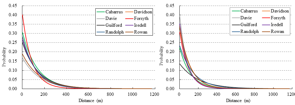
Utility functions of land owner agents can be calibrated by fitting with empirical land conversion data in each county in terms of distance to nearest urban land cover. In this study, we used the land conversion data from 2001-2006 to calibrate the utility functions of land owner agents in each county. Table 2 and Figure 4 report the calibration results of distance-decayed coefficients for each county. The calibrated distance-decayed model for land owner agents in each county of our study region is normalized—i.e., the utility of a land owner agent is the probability that the agent will sell his/her land for residential development. In this study, we use the 95% confidence intervals of the fitted coefficients to represent the pool of decision rules of land owner agents, which becomes Equation 3:
| $$D(j)=\{(\alpha_{ijk}, \beta_{ijk}) \, | \, \alpha_{ijk}\in CI\bigl(\hat{\alpha} (j,k)\bigr), \beta_{ijk} \in CI\bigl(\hat{\beta}(j,k)\bigr)\}$$ | (3) |
| County | Forest/natural to urban conversion | Farmland to urban conversion | ||
| α | β | α | β | |
| Davie | 1.7765 (1.159-2.394) | 0.0065 (0.005-0.008) | 0.927 (0.303-1.551) | 0.0123 (0.010-0.015) |
| Forsyth | 0.9164 (0.331-1.501) | 0.0114 (0.010-0.013) | 1.1802 (0.918-1.442) | 0.0107 (0.010-0.011) |
| Davidson | 1.2761 (0.967-1.585) | 0.0081 (0.007-0.009) | 1.0732 (0.621-1.525) | 0.0092 (0.008-0.010) |
| Cabarrus | 1.1836 (0.811-1.556) | 0.0075 (0.007-0.008) | 1.5109 (1.209-1.812) | 0.0085 (0.008-0.009) |
| Randolph | 1.2610 (0.806-1.716) | 0.0082 (0.007-0.009) | 1.4565 (1.030-1.883) | 0.0068 (0.006-0.008) |
| Rowan | 1.6682 (1.144-2.193) | 0.0064 (0.005-0.008) | 1.1050 (0.468-1.742) | 0.0091 (0.007-0.011) |
| Guilford | 1.3883 (1.154-1.622) | 0.0069 (0.006-0.007) | 1.9971 (1.778-2.216) | 0.0050 (0.005-0.005) |
| Iredell | 1.3257 (0.934-1.718) | 0.0076 (0.007-0.009) | 1.0430 (0.563-1.523) | 0.0118 (0.010-0.013) |
Land developers
Land developers lead on converting lands into residential area (i.e., urban land cover). In this model, we used a patch-based approach to represent the conversion of lands—each land development event by a land developer leads to the occurrence of a new patch of residential area. This patch-based approach has been used in the literature for land change simulation at a fine spatial scale (Aquilue et al. 2017; Li et al. 2017; Liu et al. 2014; McGarigal et al. 2018; Meentemeyer et al. 2013). The behavior of a land developer for land conversion consists of three major steps: 1) search for the initial location of residential development, 2) determine the area of the residential development, and 3) generate a patch of land development to realize the land conversion.
The first step of decision making associated with land development for a land developer agent is to determine where to acquire a land for residential development. Specifically, a land developer agent will randomly inspect a land that is feasible for residential development (i.e., farmland or forest/natural). The land developer decides if a land will be chosen for development based on the development probability of the land derived from his/her utility function (discussed next). A land with higher development probability is more likely to be selected. In this study, those areas that are water bodies, wetlands, or protected areas are excluded (i.e., these areas are infeasible or prohibited for land conversion). Once a land is selected, the land developer agent decides whether he/she will acquire the land for residential development using his/her utility function. The decision of a land developer on whether to acquire a land for residential development or not is a binary variable (two actions; 1: acquire; 0: do not acquire). This decision is dependent on the composite influence of a set of driving factors. In this study, the utility function of a land developer agent to acquire a land for development is based on a logistic regression model, which is represented as in the following equations (Equation 4 and 5):
| $$\it{u\_developer}(i,j) = (1+e^{-y(i,j)})^{-1}$$ | (4) |
| $$y(i,j) = \beta_0(j) + \beta_1(j)x_1+\dots+ \beta_m(j)x_m$$ | (5) |
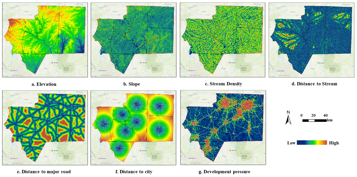
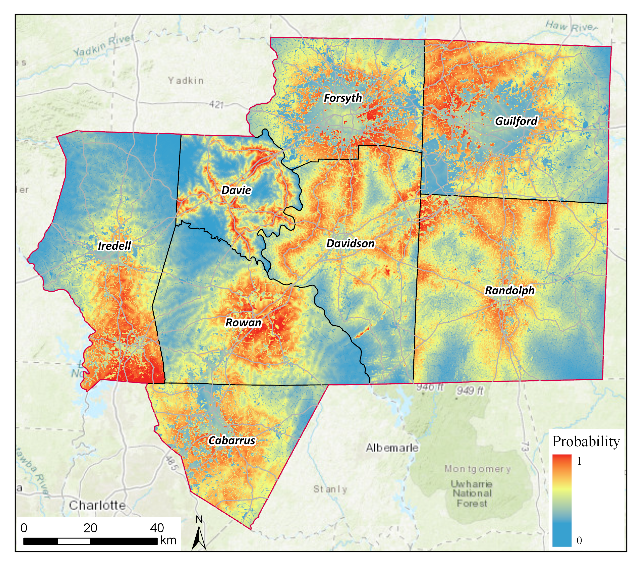
In this study, the factors that drive the decision of land developers include elevation, slope, distance to cities, distance to major roads, distance to streams, stream density, and development pressure (see Figure 5). Neighborhood size for the calculation of development pressure (the percentage of urban cover) is 35 by 35 cells. A search radius of 500 meters was used to derive stream density. For each county, the size of samples to fit the logistic regression model is 2,000 (1,000 for urban, 1,000 for nonurban) and stratified random sampling scheme was used. Land developer agents in a county share the same utility function calibrated using empirical land change data in the county from 2001 to 2006. Figure 6 shows the map of utility values (development probability) of land developers in the study region.
Once the land developer decides to acquire the land, he/she will contact the owner of the land (a land owner agent). The land owner will decide whether to sell lands to the developer or not. Only the land owner agent agrees on land transaction, the land developer can launch residential development (i.e., conversion into urban land cover type) and this land is used as the initial location of the new patch of residential development.
The second step of land conversion for a land developer agent is to determine the area of the new patch of development. The area of the new patch of development is randomly drawn from empirical area distribution of new patches of development from 2001 to 2006. In this study, we use the observed patch of change of the entire study region from 2001 to 2006 to derive the empirical distribution that a land developer agent will use to determine the area of new patch of development.
Once the initial location and area of residential development are determined, the land developer agent will generate the new patch of development. A patch growing mechanism is used to form the new patch: neighboring lands (cells) are recursively added into the new patch until the patch area is reached. The probability that a neighboring land cell is added into the development patch is the composite utility that the land developer agent decides on land acquisition multiplied by the land owner agent’s utility on land transactions at that cell. A first-order von Neumann neighborhood rule is used to search for neighboring cells during the process of forming a new patch of development.
Implementation
The code of this agent-based model was written in C/C++ programming language. All GIS data were processed in ESRI ArcGIS Pro version 2.1.3. All distance-based variables were calculated using the Euclidean distance tool in ArcGIS. All the raster GIS data were imported into the agent-based model—i.e., a loose coupling of agent-based modeling with GIS (Brown et al. 2005b). The ABM was deployed on a high-performance computing cluster (total number of CPUs: 2,060; Redhat Linux-based) for acceleration of Monte Carlo runs of the ABM. The task scheduler for high-performance computing on the Linux cluster is PBS/TORQUE. We used Shell scripts to automate the execution of the ABM and the post-processing of simulation results.
Experiments and Discussion
Our agent-based land change model allows us to explore the impact of LULCC activities on water quality in the study region. In this section, we design two experiments to explore the impact of macro- and micro-level LULCC activities on the spatiotemporal pattern of water quality at sub-watershed scale. The first experiment focuses on macro-level LULCC activities by the manipulation of annual land development demand. In the second experiment, land owners’ preference on land transactions was varied to represent LULCC activities at micro or individual level. We first discuss performance metrics and model calibration and validation before we present the design and results of the two experiments.
Performance metric
We used bivariate similarity metrics that are based on confusion matrix to evaluate the agreement between simulated and reference land cover patterns. A variety of similarity metrics based on confusion matrix have been developed in the literature. These similarity metrics include percent correct match, figure of merits, Kappa coefficients, producer accuracy, and user accuracy (Fielding & Bell 1997; Pontius 2002). While these metrics are limited to categorical variables and the cell level (instead of object level), they provide support for the evaluation of locational agreement between simulation outcome and observed patterns. Further, these similarity metrics only provide an overall evaluation for a study region of interest based on cell-level comparison. Thus, often time, a study region is partitioned into a collection of sub-regions (e.g., using lattice with coarser spatial resolutions) when using these metrics to evaluate the agreement between simulation outcome and reference patterns (Kok et al. 2001; Pontius 2002). In this study, we used two percent correct match indices (\(\textit{pcm}_1\) and \(\textit{pcm}_2\)) that are based on confusion matrix (Pontius et al. 2008; Pontius & Millones 2011; van Vliet et al. 2016), shown in the following equations (Equation 6, 7).
| $$\textit{pcm}_1=\frac{n_a}{n_a+n_b}$$ | (6) |
| $$\textit{pcm}_2=\frac{n_a+n_d}{n_a+n_b+n_c+n_d}$$ | (7) |
Model calibration and validation
Model calibration and validation are important steps of land change simulation modeling (Brown et al. 2005a; van Vliet et al. 2016). In general, there are two approaches for model calibration and validation: partitioning of temporal duration or spatial extent of a study system into calibration set (period or area) and validation set that do not overlap with each other (Pontius et al. 2004a). A model is instantiated using data in the calibration set for the specific study region of interest. Simulation outcome of the calibrated model is compared with data in the validation set to ensure the model has sufficient predictive power (instead of being overfitted to calibration data) and thus is valid for experimentation use. Typically, temporal partitioning is often used for land change modeling given the availability of land cover data and related data over time. The simulation period of a model is divided into calibration period and validation period. In this study, the calibration period is from 2001-2006, and the validation period is from 2006 to 2011. The utility functions (the distance-decayed model) of land owners were calibrated using the land conversion data from 2001-2006 in each county. The utility function of land developers in a county was calibrated using logistic regression based on empirical land change data in the county from 2001 to 2006. We used the area of land conversion from 2001 to 2006 in each county to represent the annual land development demand during the calibration phase. Please see the ODD protocol of our ABM in the Appendix for more detail.
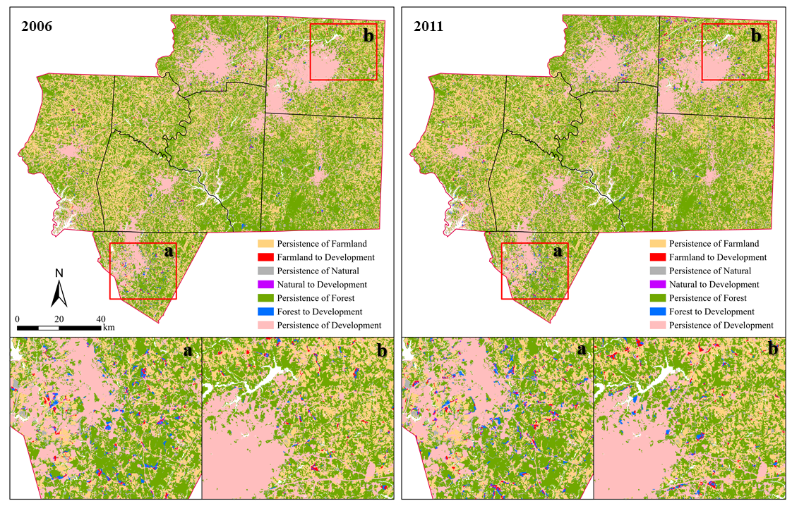
Figure 7 shows the maps of simulated land cover patterns for year 2006 and 2011. These maps depict the spatial patterns of persistence and change of land cover types. From these maps, we can see that most of farmland and forest land cover remain persistent over time—i.e., the landscape of our study region is dominated by persistence. The simulation accuracy of \(\textit{pcm}_1\) for 2001-2006 (calibration accuracy) is 4.32% on average (with a standard deviation of 0.43%; based on 100 Monte Carlo runs). The corresponding simulation accuracy in terms of \(\textit{pcm}_2\) is averaged at 96.90% (std: 0.02%).
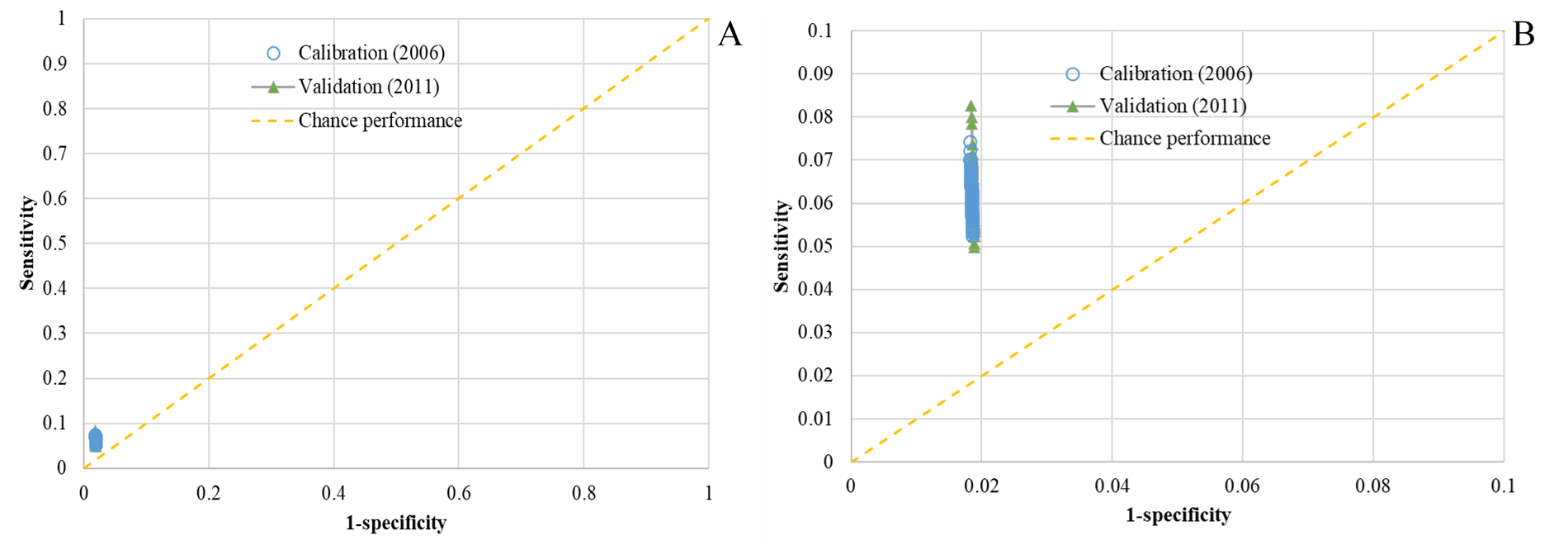
We ran our simulation model to 2011 for validation purpose. Annual land change demand from 2006 to 2011 was based on the empirical land change quantity during this period. The validation accuracy \(\textit{pcm}_1\) is 6.56% on average (std: 0.49%). The averaged \(\textit{pcm}_2\) is 96.26% (std: 0.03%) for the validation period. The simulation accuracy in terms of \(\textit{pcm}_1\) (\(\textit{pcm}_2\)) is low (high) because land change quantity during the two simulation periods only occupies about 1-1.5% of the study area and most of the regions do not experience land change (i.e., high-level persistence; see Figure 7). Increase in simulation accuracy in terms of \(\textit{pcm}_1\)is partially attributed to the occurrence of more land development from 2006 to 2011 (Pontius et al. 2008). Figure 8 depicts the receiver operating characteristic (ROC; see Pontius & Schneider (2001) and Fielding & Bell (1997)) plot of our agent-based model for calibration and validation runs (100 runs for each). The ROC plot suggests that while our model accuracy in terms of \(\textit{pcm}_1\) is low, the model performance is acceptable by comparing with the performance due to chance (the performance of all model runs for calibration and validation is higher than chance performance in the ROC plot).
While low net land change or high-level persistence explains low simulation accuracy of our model (Pontius et al. 2008; Pontius et al. 2004b), of more interest is the variation of simulation accuracy across our study region. Thus, we extracted sub region-level accuracy using a grid with coarser spatial resolution (3km by 3km here). Figure 9 shows the spatial distribution of averaged accuracy (pcm1) for calibration and validation phases at sub region level. As we could see, the averaged simulation accuracy varies from 0-17.66% for 2001-2006 (calibration period), and can reach up to 26.14% for the simulation period of 2001-2011 (validation period). For rural areas (e.g., Davie, Randolph, Rowan Counties), simulation accuracies are low (even reach zero hits because the development probability calibrated using historical data in these rural areas is low). High simulation accuracies tend to concentrate in urban areas (e.g., those in Cabarrus, Forsyth, Guilford, and Iredell Counties). Those urban areas typically have high net land change, which is likely to have reasonably high accuracies as indicated in the literature (Pontius et al. 2008). The accuracy assessment results suggest that our ABM provides reasonable support for the simulation of land development in our study region (most developments typically concentrate in urbanized areas) and thus empowers the exploration of the relationship between LULCC and water quality.
Experiment of land development demand at macro level
In this experiment, we aim to explore the impact of alternative land development demand on the water quality at the sub watershed level in our study region. We use the annual land development demand derived from empirical land change data from 2001 to 2006 as a baseline scenario. We vary the annual land development demand at the county level by 20%, 60%, 100%, 140%, and 180%. Correspondingly, we have five treatments (\(T_1\), \(T_2\), \(T_3\), \(T_4\), and \(T_5\)) for this experiment. For each treatment, the agent-based simulation model ran from 2001 to 2040. Each treatment was repeated 100 Monte Carlo runs. These treatments were designed to represent different land development scenarios. The first two treatments are designed to represent the scenarios of slow land development, and treatment \(T_4\) and \(T_5\) for the scenarios of rapid land development.
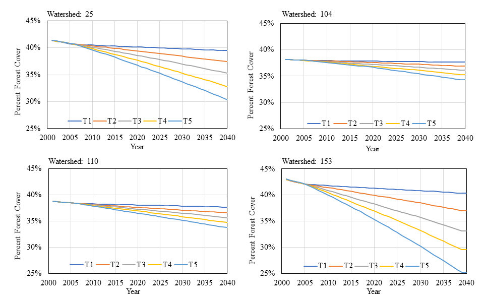
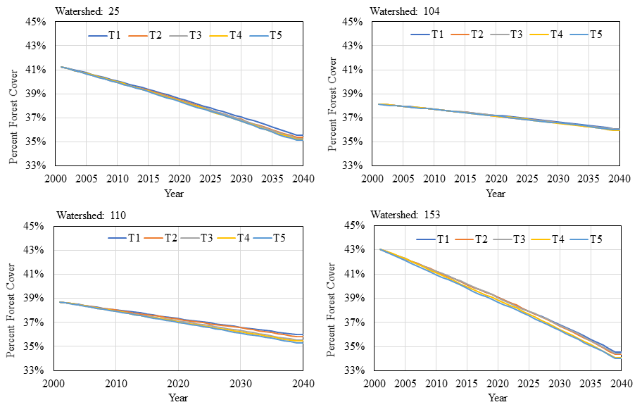
Figure 10 shows the maps of water quality patterns at sub watershed level for the five treatments. Table 3 reports the number of sub watersheds falling within the three types of water quality states (good, fair, and poor). Figure 11 illustrates the time series of percent in forest cover over years for four sub watersheds. A sub watershed belongs to good or poor water quality states only when it remains in the same state for all 100 simulation runs (otherwise, it belongs to the category of fair water quality—i.e., within the threshold). As we could observe, the number of sub watersheds with good water quality decreases (from 56 to 34) when land development demand increases. In other words, more sub watersheds (from 71 to 93) fall within the critical threshold (fair water quality). The average number of years that these critical sub watersheds remain its state is 31.79, 29.06, 25.66, 23.91, and 21.75 for the five treatments. It shows that increment in the quantity of land development tends to reduce the length of the time that critical sub watersheds remain in the same state.
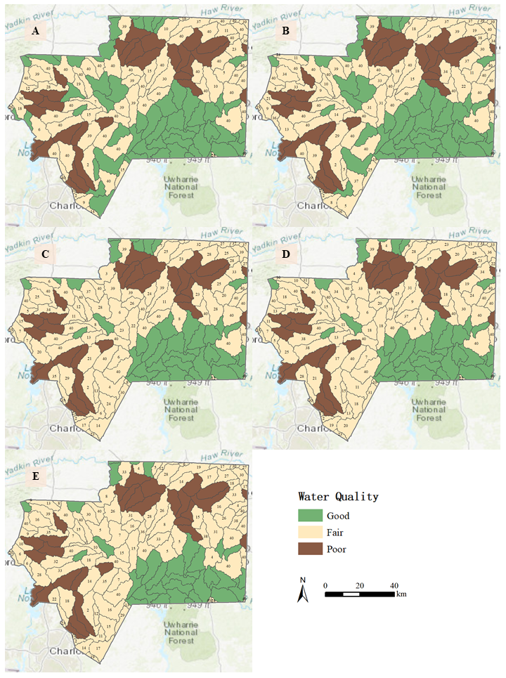
| Water quality | T1 | T2 | T3 | T4 | T5 |
| Good | 56 | 49 | 42 | 38 | 34 |
| Fair | 71 | 78 | 85 | 89 | 93 |
| Poor | 32 | 32 | 32 | 32 | 32 |
Experiment of land owner preference at micro level
The second experiment is to evaluate the influence of land owner’s preference on water quality in the study area. In this model, the land owners’ preference is associated with the decision pool of utility functions characterized by distance-decayed models (see Equation 1). Distance-decayed coefficients (\(\alpha_{ijk}\), \(\beta_{ijk}\)) in the decision pool with respect to conversion from forest or natural lands to urban were systematically varied by adding a specific amount of change (\(\sigma\ast r(\alpha_{ijk})\), \(\sigma\ast r(\beta_{ijk})\)), where \(r(.)\) is the range of the corresponding coefficients (see Equation 3). Utility functions of land owner agents on farmland to urban conversion remain unchanged. We design five treatments (\(T_1\)-\(T_5\)) by assigning \(\sigma\) to 1.0, 0.5, 0, -0.5, and -1.0 correspondingly. We ran our model from 2001 to 2040 for each treatment. The number of Monte Carlo runs for each treatment is 100.Varying distance-decayed coefficients will modify the shape of the distance-decayed curves: high coefficients will render that the magnitude of the utility becomes lower and the distance-decayed curve becomes steep. In other words, land owner agents with high distance-decayed coefficients tend to have low preference on selling their forest or natural lands for residential development.
Table 4 reports the simulation results in terms of the number of sub watersheds at different states. Figure 12 shows the maps of water quality patterns across the five treatments. Figure 13 illustrates change in the percentage of forest cover of four sub watersheds. In general, we could observe a decreasing pattern in terms of the number of sub watersheds with good water quality when distance-decayed coefficients that evaluate land owner agents’ preference on land development become lower (corresponding to high utility values of selling their forest land). The average number of years that critical sub watersheds (fair water quality) remain their states is 26.41, 26.36, 25.90, 26.04, and 25.96 for the five treatments. The number of years that a sub watershed stays within the critical threshold tends to be shortened as distance-decayed coefficients become lower (from 26.41 years to 25.96 years). This means that land owner agents with higher preference on selling their forest lands for development tend to accelerate the state transition of critical sub watersheds (from fair to poor water quality).
Discussion
The quantity of land development functions as a top-down mechanism that drives LULCC in a study region. Variation in land development demand (e.g., due to change in economy or population) is of pivotal importance in affecting the sub watershed-level water quality in our study region. As increase in land development demand, more sub watersheds with good water quality will transit to the critical threshold state, as indicated by the first experiment. Further, the length of the time that critical sub watersheds remain their states is reduced in response to increased land development demand. This is because land developments at sub-watershed level will generally occur more in response to increased annual demand for land development at county level. More land development events consume more forest lands, leading to the detrimental effect on water quality (see Figure 11). In particular, if we remain the land develop demand same as that between 2001 and 2006 (baseline scenario), within 25.66 years from 2001 (i.e., around year 2026) all sub watersheds in our study region will tend to shift their states (from fair to poor water quality) in general. However, this transition time will be delayed if policies or regulations that control the number of land development events are adopted by, for example, government agencies. In particular, experimental results (the first experiment) suggest that gain in the delayed time of transition due to regulated land development (6.13 years for 80% of reduction in development demand) is higher than loss in the transition time resulting from increased land development (3.91 years for 80% increment in demand). This implies the importance of land conversation policies in the protection of water quality in watershed ecosystems.
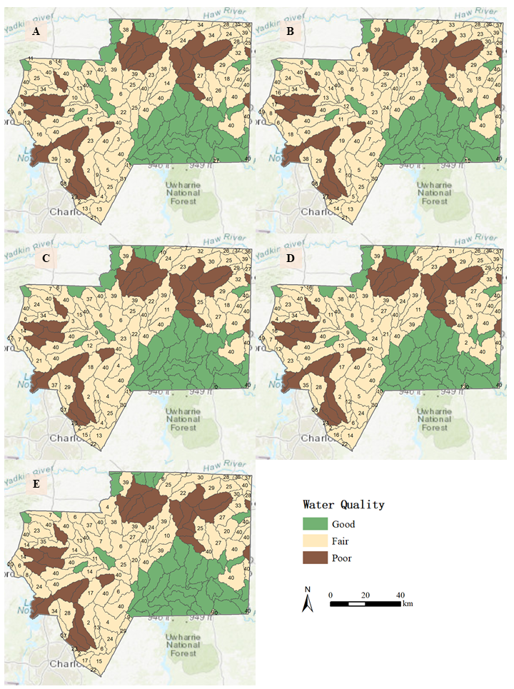
| Water quality state | T1 | T2 | T3 | T4 | T5 |
| Good | 46 | 45 | 45 | 45 | 44 |
| Fair | 81 | 82 | 82 | 82 | 83 |
| Poor | 32 | 32 | 32 | 32 | 32 |
Human decision-making processes and subsequent choices often play a fundamental role in driving the landscape dynamics of watershed ecosystems that are modified by human actors. Our experimental results (the second experiment) demonstrate this role of human decision-making. Change in coefficients of utility functions of land owners (based on distance-decayed models) correspond to a continuum from organic land development (high values) to spontaneous development (low values) (Liu et al. 2017; Liu et al. 2014; Torrens 2006). Varied preference of land owners may lead to alternative landscape patterns in terms of watershed conditions such as water quality here. This suggests the necessity of environmental education in terms of water quality protection for decision-makers involved in land development (Giri & Qiu 2016). Environmental education, possibly together with incentives from governments or institutional efforts on land conservation, will increase the awareness of decision makers in the potential negative effect of land development on the water quality of residents’ living environments. This will warrant the sustainability of watershed ecosystems shaped by land development.
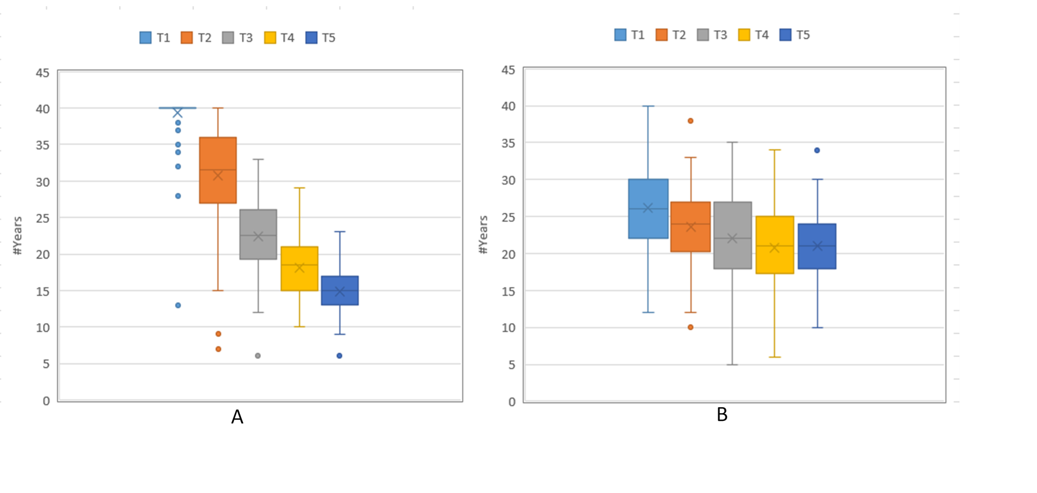
Further, the critical threshold of water quality driven by LULCC in this study is similar to (or can be explained as) relaxation phenomena (Malanson 2008), in which time-delayed effect exists between the occurrence of an event (e.g., disturbance, stress, or land development here) in a system and response of the system to that event (e.g., change in water quality in this study). The temporal transition patterns of system states are so-called relaxation paths, which are driven by the strength of the event (land development in this study) and the capability that the system adjusts its states to equilibriums (different water quality states in this study). The time that a system stays within the relaxation phase is relaxation time. In our model, the relaxation time of a sub watershed is the number of years it will maintain the state of fair water quality. Figure 14 depicts the distribution of the relaxation time of a specific sub watershed in our study region for the two experiments. As we could observe, the relaxation time of this specific sub watershed tends to be shortened as land development demand (macro level) increases or land owner agents have more preference on land transactions for development (micro level). This shortened relaxation time pattern can be observed for many sub watersheds with initial state of fair water quality (see Figure 10 and 12). However, for sub watersheds in which initial water quality state is good, the relaxation time tends to be delayed in response to increased land development demand and higher agent preference on land transactions. This is because it takes some time for sub watersheds to transit from the good water quality state to fair and this amount of time is shortened for higher development demand or higher preference of land owner agents. As a result, the relaxation time, which corresponds to the number of years sub watersheds stay at the fair water quality state, is longer for higher development demand or higher individual-level preference. Thus, we can see that the agent-based land change model together with the forest cover model of water quality provides substantial support for the exploration of the relaxation effect in terms of the impact of LULCC on water quality in this study. This will be of great help in terms of developing a promoted understanding of the spatiotemporal complexity of watershed ecosystems.
Conclusion
In this study, the agent-based land change model was developed to enable investigations on the relationship between LULCC and water quality in eight NC counties. Our study area covers the lower High Rock Lake Watershed region. The agent-based model was designed within a demand-allocation framework, including modules of land demand and spatial allocation. Two types of agents, land owners and land developers, were used to represent the decision-making processes involved with land development. Land owners have preference on selling their lands for land development, which is represented using distance-decayed modeling. Land developers interact with land owners and decide where and how to realize their needs of land development. Interactions between land owners and land developers produce a complex landscape of land development, which inherently drives spatiotemporal patterns of water quality at sub-watershed level in our study region.
The contribution of this article is the use of agent-based modeling approach to investigate the space-time locations of critical threshold of water quality driven by land use and land cover change at various decision levels (macro and micro). Critical threshold or threshold effect is a representative property of complex coupled human and natural system (Liu et al. 2007a). However, studies on where and when threshold effects may occur are inadequate in the literature. The work reported in this article has unique contribution to this thread, particularly, the study of space-time locations of critical threshold within the context of land use and land cover change. The water quality of sub watersheds in this study is represented by a forest cover model, which uses a threshold of 37-48% of percent forest cover that classifies sub watersheds into different states (three: good, fair, and poor water quality). Spatiotemporally explicit land development modifies land cover patterns, which consequentially lead to the transition of water quality in sub watersheds into different states. In particular, those sub watersheds within the threshold are of more interest in terms of the protection of water quality. These sub watersheds experience transient dynamics (Malanson 1999, 2008) that serve as a buffer state of transition between good and poor water quality (most of the time, from good to poor water quality). Our experiments indicate that the length of the transition phase, also known as relaxation time, is influenced by land development at different decision scales (macro-level: land change demand; micro-level: land owner preference). The agent-based land change model enables us to conduct alternative what-if scenario analysis that helps identify complex spatiotemporal patterns of sub watersheds experiencing critical thresholds. Further, the agent-based modeling approach is necessary (and preferred over other modeling approaches such as cellular automata or system dynamics models) because of its ability to supporting explicit representation of decision-making processes of individuals (land owners and land developers here) that are often heterogeneous and uncertain. This allows us to investigate the impact of individual-level behavior on macro-level system response (watershed-level water quality here).
Our agent-based land change model provide efficacious support for the exploration of complex relationship between LULCC and water quality in watershed-level ecosystems. Future work may focus on the following threads. First, we will apply this ABM to other study regions which may have alternative ecoregions (e.g., coastal plain or mountain) to further examine its utility in representing LULCC and associated spatiotemporal patterns of watershed conditions. Second, our current ABM has limitations in the representation of adaptive behavior of decision- or policy makers. Thus, in the future work, we plan to integrate machine learning approaches with the agent-based model so as to identify optimal or adaptive land conservation strategies, which will greatly support policy makers to prioritize regions in need of, for example, water quality protection. Machine learning approaches such as evolutionary algorithms, neural networks, swarm intelligence, and reinforcement learning hold great promise for the representation of adaptation in land systems (Bone & Dragićević 2010; Tang 2008) and will be used to explore the influence of adaptation in decision making of individuals and policy making of government agencies (e.g., for local government planning) on ecosystem-level response. Further, machine learning approaches can be of great help in the calibration and validation of agent-based modeling (e.g., use of neural networks for calibration of land developer’s decision instead of logistic regression; see Pijanowski et al. 2005). Third, our ABM is an integration of agent-based approach, cellular automata, and distance-decayed models together with a set of parameters and input data. In future studies, we will conduct sensitivity analysis and uncertainty analysis to evaluate the relationship between uncertainties in model input or structure and uncertainties in model outcome. This will be of great help in minimizing the occurrence of possible structural mistakes and misspecification of our ABM (O'Sullivan et al. 2016). Fourth, the agent-based land change modeling is computationally demanding, in particular, for the experimentation of scenario analysis. Thus, a parallel computing solution of the agent-based land change model will be developed to accelerate model execution by leveraging high-performance computing power from cutting-edge cyberinfrastructure (NSF 2007; Tang & Jia 2014; Tang et al. 2011).
Model Documentation
This model was implemented in C++, based on the modification of an agent-based simulation platform, GAIASP (Tang 2008). The code of the model is available online here: https://github.com/wenwu-tang/agentlcm.Acknowledgements
The authors thank North Carolina Forest Services for the water quality data through a contract agreement. University Research Computing (URC) at the University of North Carolina at Charlotte provides high-performance computing resources for the development and experimentation of the agent-based land change model in this study. The authors owe thanks to anonymous reviewers for their comments. The authors contributed equally to the work presented in this article.Appendix: The Overview, Design concepts, Details (ODD) Protocol
In this supplementary material, we document our agent-based model (ABM) using the ODD protocol by Grimm et al. (2010).
Purpose
Our ABM aims to simulate land changes in a large watershed (the lower High Rock Lake Watershed, HRLW, in North Carolina, USA), thus to identify the space-time locations of potential regions (sub watersheds) that may experience critical threshold of water quality.
Entities, state variables, and scales
There are two types of agents in the model: land owners and land developers. Both land owners and land developers are hypothetical agents situated within each county. Also, we assume each land unit (grid cell here) that is covered by farmland, forest, or natural land is managed by a land owner agent, and can be aquired by a land developer for residential development. Land developers are in charge of decision making in terms of where, how, and how many to acquire land for development based on his/her utility function represented by a logistic regression model. The land owners decide whether to sell their lands for development based on his/her perception on surrounding environments when contacted by a land developer. The utility function of a land owner agent to sell land is represented using a distance-decayed model.
The grid cells in the watershed serve as spatial context where land owners and land developers interact with each other. The state variables of land owners, land developers, and grid cells are listed in Table 5
One time step in the model represents one year in reality. We ran the model for 40 years which covers three periods: 2001-2006 for parameters calibration, 2006-2011 for model performance validation, and 2011-2040 for scenario-based future projection. The spatial resolution of the raster grid is 30m \(\times\) 30m, resulting in 4,378 rows and 4,746 columns in the landscape of interest.
| Symbol | Description (unit) | Value |
| Grid cell | ||
| \(k\) | Land cover type | Farmland, forest, natural, water, urban |
| (\(x\), \(y\)) | Coordinate of the grid cell (m) | |
| \(x_1\) | Elevation (m) | |
| \(x_2\) | Slope (%) | |
| \(x_3\) | Stream density (m/m2) | |
| \(x_4\) | Distance to stream (m) | |
| \(x_5\) | Distance to major road (m) | |
| \(x_6\) | Distance to city (m) | |
| \(x_7\) | Development pressure | |
| Land owner agent | ||
| \(i\) | Identifier of the land owner agent | |
| \(j\) | Identifier of county that land owner agent located in | [1, 8] |
| \(\alpha(i,j,k)\) | Coefficient that controls magnitude of the utility of the land owner agent \(i\) in county \(j\) with respect to the land cover type k of his/her land parcel | |
| \(\beta(i,j,k)\) | Coefficient that is associated with the steepness of the distance-decayed function representing the utility of land owner agent \(i\) in county \(j\) with respect to the land cover type \(j\) of his/her land parcel | |
| \(\it{u\_owner}(i,j,k)\) | Utility of land owner agent \(i\) in county \(j\) with respect to the land cover type \(j\) of his/her land parcel | [0, 1] |
| Land developer agent | ||
| \(B_{0(j)}\), \(B_{1(j)}\),\(\dots\),\(\beta_{m(j)}\) | Coefficients for the corresponding driving factors in county \(j\) | |
| \(\it{u\_developer}(i,j)\) | Utility of a land developer agent i in county \(j\) | |
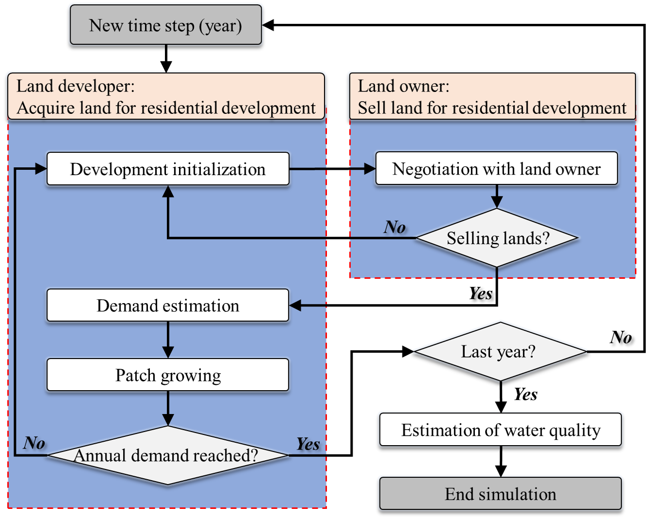
Process overview and scheduling
The time step is one year in our ABM. The model starts from 2001 and run into 2006 for model calibration, to 2011 for model validation, and to 2040 for future projection under different scenarios. The overall processes in the ABM are presented in Figure 15. These processes mainly include 1) acquire land for residential development, which includes four major steps: development initialization, negotiation with land owner, demand estimation, and patch growing; 2) sell land for residential development; and 3) estimation of water quality.
Design concepts
Basic principles
The model is the spatial representation of the urban development process in real-world, which involves the decision-making of land developers and land owners, as well as their direct and indirect interactions. In this study, we focus on the land conversion process from farmland, forest, and natural land to urban land. A land developers decide on whether to acquire a feasible land for residential development based on his/her utility function which is calculated from a set of driving factors using a logistic regression model. A land owner can be contacted by a land developer, and make his/her own decision on whether to sell land for development based on his/her utility function which is a distance-decayed abstraction of the surrounding environments.
Emergence
The spatial pattern of residential development in the lower HRLW, especially in each sub watershed, emerges from the interactions between land developer agents and land owner agents. The results of residential development in the previous period update the surrounding environment of agents, thus influencing their decision-making in subsequent steps.
Adaptation
The utility of land developer is an adaptive trait changing along with consecutive residential development activities in surrounding environments. So does the utility function of the land owners.
Objectives
Land owners closer to existing urban areas have higher utility of land conversion, thus more likely to sell their lands. Also, lands with more residential development in surrounding environment are more likely to be converted by land developers.
Learning
The ABM involves no learning attributes.
Prediction
The ABM involves no prediction attributes.
Sensing
Land developer agent can sense the state variables of grid cells that he/she intends to convert for estimating his/her utility. Land owner can sense the location and land cover type of the land that he/she manages, as well as the surrounding residential development, thus to calculate distance to nearest development areas in order to estimate his/her utility of selling land.
Interaction
Land developer has to directly contact a land owner to ask whether the owner will sell his/her land for residential development. Second, the spatial pattern of residential development emerging from interactions between land developers and land owners can influence their decision-making, which indicates indirect interactions between agents through the shared environment.
Stochasticity
First, there is a collection of utility functions of land owner agents in a county, which represents the heterogeneity of agent decision-making. For a specific land owner agent, his/her utility function is randomly drawn from the decision pool of land owner agents in the county. Second, the land selling process is stochastic. A random probability is drawn and compared against the utility value of the land owner agent to decide whether he/she will sell the land. Third, a land developer agent conducts a random inspection to find a land that is feasible to initialize a residential development activity. Fourth, the area (or size) of the new patch generated by land developer is randomly drawn from empirical distribution of area of new development patches from 2001 to 2006. Fifth, during the patch growing process, whether a neighboring cell will be added into the new patch is determined stochastically, based on a composite utility that is the multiplication of the utility of a land developer and that of a land owner with respect to the neighboring cell.
Collectives
A patch which indicates an urban land parcel in real-world is a collective of grid cells, whose area is randomly drawn from observed distribution of new patches generated by historical development activities.
Observation
In each time step, the model observes the total amount of lands that are converted to urban in each county. At the end of the simulation, the model records the percent of forest and urban cover in each sub watershed to estimate the state of water quality.
Initialization
The ABM started from 2001 and ran to 2006 for model calibration and to 2011 for model validation. The total area of our study region is 10,823 km2 with size of 4,378×4,746 in terms of number of rows and columns. The region is administrated by 8 counties and is divided into 159 sub watersheds. Each grid cell covered by farmland, forest, or natural is assumed to be managed by a land owner agent. The collective of utility functions (the distance-decayed model) of land owners was calibrated using the land conversion data from 2001-2006 in each county. Land developers lead on the residential development process in each county. The utility function (the logistic regression model) of land developers in a county was calibrated using empirical land change data in the county from 2001 to 2006. The factors used to fit the logistic regression model include elevation, slope, distance to cities, distance to major roads, distance to streams, stream density, and development pressure. Neighborhood size for the calculation of development pressure is 35 by 35 cells. A search radius of 500 meters was used to derive stream density. The size of samples to fit the logistic regression model is 2,000 (1,000 for urban, 1,000 for nonurban) in each county and stratified random sampling scheme was used. We use the observed patch of change of the entire study region from 2001 to 2006 to derive the empirical distribution that a land developer agent will use to determine the area of new patch of development. We used the area of land conversion from 2001 to 2006 in each county to represent the annual land development demand during the calibration phase.
Input data
Three years (2001, 2006, and 2011) of land cover data were used to calibrate and validate the ABM, including the utility functions of land developers and land owners, and the structure of the ABM. Data of road and stream networks, locations of cities or towns, and DEM were used to calculate the factors that impact decisions of land developer agent. The spatial extent of HRLW, the sub watersheds in this region, and the county boundaries were from the USDA National Hydrography Dataset. The land cover data were retrieved from U.S. National Land Cover Database (NLCD). Elevation data is from NASA SRTM data.
Submodels
(1) Acquire land for residential development:
The process of acquiring land for residential development consists of four major steps:
1) Development initialization
The land developers initialize the acquisition of land for residential development by searching for an initial location that is feasible under the guidance of his/her utility function. The utility function was derived through a logistic regeression analysis between historical residential development activities and a set of driving factors, which can be represented as in the following equations:
| $$\it{u\_developer}(i,j) = (1+e^{-y(i,j)})^{-1}$$ | (8) |
| $$y(i,j) = \beta_(j)+ \beta_1(j)x_1+\dots+ \beta_m(j)x_m$$ | (9) |
Land developer agents in a county share the same utility function calibrated using empirical land change data in the county from 2001 to 2006. Specifically, a land developer agent inspect a land that is feasible for conversion in a stochastic manner (based on the development probability of the land). In this study, those areas that are water bodies, wetlands, or protected areas are excluded from development.
2) Negotiation with land owner
Once the land developer selects a feasible initial location (a grid cell) for development, he/she has to contact the land owner dwelling in this cell to negotiate about the selling of the land. The land owner will decide whether to sell the land for residential development based on his/her utility. If the land owner agrees to sell the land, then the land developer will initialize a new patch of residential development with sepecified area from this location.
3) Demand estimation
If the land developer and the land owner reach an agreement on initializing a residential development activity, the land developer will specify the amount of land conversion, i.e. the area of the new patch. In this study, the area of the new patch is randomly drawn from a pool of patch size derived from the observed patches of change of the entire study region from 2001 to 2006 (calibration period).
4) Patch growing
A patch growing mechanism is used to form the new patch with speicfied area: neighboring lands (cells) are iteratively added into the new patch until the specified patch area is reached, or the annual demand of residential development in a county is satisfied. Similarily, each time a new cell is to be included in the new patch, the land developer has to negotiate with the land owner. In other words, the probability that a neighboring land cell is added into the development patch is the composite utility that the land developer agent decides on land acquisition multiplied by the land owner agent’s utility on land transactions at that cell.
(2) Sell land for residential development
The land owner decides whether to sell his/her land (including farmland, forest, and natural in this study) during the negotiation with land developer according to the utility from land transaction. The utility function is represented by a distance-decayed model, which is formulated as follow:
| $$\it{u\_owner}(i,j,k)=e^{-\alpha(i,j,k)} e^{–\beta(i,j,k)\ast d}$$ | (10) |
| $$D(j)=\{(\alpha_{ijk}, \beta_{ijk}) \, | \, \alpha_{ijk}[\alpha_{ljk}, \alpha_{hjk}], \beta_{ijk}[\beta_{ljk}, \beta_{hjk}]\Bigr\}$$ | (11) |
| $$ D(j)=\{(\alpha_{ijk}, \beta_{ijk}) \, | \, \alpha_{ijk} \in CI\bigl( \hat{\alpha}(j,k) \bigr), \beta_{ijk} \in CI\bigl( \hat{\beta}(j,k) \bigr)\Bigr\}$$ | (12) |
(3) Estimation of water quality:
The water quality in the HRLW was related to the percent of forest cover in a sub watershed. The relationship was established based on an empirical analysis of five years of land cover data and benthic macroinvertebrate data. Sub watersheds with percent forest cover higher than 48% (or lower than 37%) correspond to good (or poor) water quality. Any sub watersheds with the percentage of forest cover within the range of 37-48% are at the tipping point with fair water quality that may be shifted to either good or poor states.
References
AN, L., Linderman, M., Qi, J., Shortridge, A., & Liu, J. (2005). Exploring Complexity in a Human–Environment System: An Agent-Based Spatial Model for Multidisciplinary and Multiscale Integration. Annals of the Association of American Geographers, 95(1), 54-79. [doi:10.1111/j.1467-8306.2005.00450.x]
AN, L., Zvoleff, A., Liu, J., & Axinn, W. (2014). Agent-based modeling in coupled human and natural systems (CHANS): lessons from a comparative analysis. Annals of the Association of American Geographers, 104(4), 723-745. [doi:10.1080/00045608.2014.910085]
AQUILUE, N., De Caceres, M., Fortin, M. J., Fall, A., & Brotons, L. (2017). A spatial allocation procedure to model land-use/land-cover changes: Accounting for occurrence and spread processes. Ecological Modelling, 344, 73-86.
BARBOUR, M. T., Gerritsen, J., Snyder, B. D., & Stribling, J. B. (1999). Rapid bioassessment protocols for use in streams and wadeable rivers: periphyton, benthic macroinvertebrates and fish (Vol. 339): US Environmental Protection Agency, Office of Water Washington, DC.
BONE, C., & Dragićević, S. (2010). Simulation and validation of a reinforcement learning agent-based model for multi-stakeholder forest management. Computers, Environment and Urban Systems, 34(2), 162-174. [doi:10.1016/j.compenvurbsys.2009.10.001]
BROWN, D. G., Page, S., Riolo, R., Zellner, M., & Rand, W. (2005a). Path dependence and the validation of agent‐based spatial models of land use. International Journal of Geographical Information Science, 19(2), 153-174. [doi:10.1080/13658810410001713399]
BROWN, D. G., Riolo, R., Robinson, D. T., North, M., & Rand, W. (2005b). Spatial process and data models: Toward integration of agent-based models and GIS. Journal of Geographic Systems, 7(1), 1-23. [doi:10.1007/s10109-005-0148-5]
COUNCIL, N., R. (2014). Advancing Land Change Modeling: Opportunities and Research Requirements: National Academies Press.
EPSTEIN, J. M., & Axtell, I. (1996). Growing Artificial Societies: Social Science from the Bottom Up. Cambridge, MA: The MIT Press. [doi:10.7551/mitpress/3374.001.0001]
FIELDING, A. H., & Bell, J. F. (1997). A review of methods for the assessment of prediction errors in conservation presence/absence models. Environmental conservation, 24(1), 38-49. [doi:10.1017/s0376892997000088]
GEROW, T. A., Jones, D. G., & Tang, W. (2015). Assessment of forest cover in the High Rock Lake Watershed. Paper presented at the Water Resource Research Institute 2015 Annual Conference, Raleigh, NC, USA.
GEROW, T. A., Jones, D. G., & Tang, W. (2016). Assessing the relationship between forests and water in the High Rock Lake Watershed of North Carolina. Paper presented at the In: Stringer, Christina E.; Krauss, Ken W.; Latimer, James S., eds. 2016. Headwaters to estuaries: advances in watershed science and management-Proceedings of the Fifth Interagency Conference on Research in the Watersheds. March 2-5, 2015, North Charleston, South Carolina. e-General Technical Report SRS-211. Asheville, NC: US Department of Agriculture Forest Service, Southern Research Station. 302 p.
GIRI, S., & Qiu, Z. (2016). Understanding the relationship of land uses and water quality in Twenty First Century: A review. Journal of environmental management, 173, 41-48. [doi:10.1016/j.jenvman.2016.02.029]
GOULD, P. R. (1969). Spatial Diffusion, Resource Paper No. 4. Washington, DC: Association of American Geographers.
GRIMM, V., Berger, U., DeAngelis, D. L., Polhill, J. G., Giske, J., & Railsback, S. F. (2010). The ODD protocol: a review and first update. Ecological Modelling, 221(23), 2760-2768. [doi:10.1016/j.ecolmodel.2010.08.019]
GRIMM, V., Revilla, E., Berger, U., Jeltsch, F., Mooij, W. M., Railsback, S. F., . . . DeAngelis, D. L. (2005). Pattern-oriented modeling of agent-based complex systems: lessons from ecology. Science, 310(5750), 987-991. [doi:10.1126/science.1116681]
GROENEVELD, J., Müller, B., Buchmann, C. M., Dressler, G., Guo, C., Hase, N., . . . Lauf, T. (2017). Theoretical foundations of human decision-making in agent-based land use models–A review. Environmental modelling & software, 87, 39-48. [doi:10.1016/j.envsoft.2016.10.008]
HAGERSTRAND, T. (1968). Innovation Diffusion as a Spatial Process. Chicago: University of Chicago Press.
HAIDARY, A., Amiri, B. J., Adamowski, J., Fohrer, N., & Nakane, K. (2013). Assessing the impacts of four land use types on the water quality of wetlands in Japan. Water Resources Management, 27(7), 2217-2229. [doi:10.1007/s11269-013-0284-5]
KAUFFMAN, G. J., & Brant, T. (2000). The role of impervious cover as a watershed-based zoning tool to protect water quality in the Christina river basin of Delaware, Pennsylvania, and Maryland. Proceedings of the Water Environment Federation, 2000(6), 1656-1667. [doi:10.2175/193864700785150132]
KOK, K., Farrow, A., Veldkamp, A., & Verburg, P. H. (2001). A method and application of multi-scale validation in spatial land use models. Agriculture, Ecosystems & Environment, 85(1-3), 223-238. [doi:10.1016/s0167-8809(01)00186-4]
LAUF, S., Haase, D., Hostert, P., Lakes, T., & Kleinschmit, B. (2012). Uncovering land-use dynamics driven by human decision-making – A combined model approach using cellular automata and system dynamics. Environmental modelling & software, 27-28, 71-82. [doi:10.1016/j.envsoft.2011.09.005]
LI, X. C., Gong, P., Yu, L., & Hu, T. Y. (2017). A segment derived patch-based logistic cellular automata for urban growth modeling with heuristic rules. Computers Environment and Urban Systems, 65, 140-149. [doi:10.1016/j.compenvurbsys.2017.06.001]
LIU, J., Dietz, T., Carpenter, S. R., Alberti, M., Folke, C., Moran, E., . . . Lubchenco, J. (2007a). Complexity of coupled human and natural systems. Science, 317(5844), 1513-1516. [doi:10.1126/science.1144004]
LIU, J., Dietz, T., Carpenter, S. R., Folke, C., Alberti, M., Redman, C. L., . . . Lubchenco, J. (2007b). Coupled human and natural systems. AMBIO: A Journal of the Human Environment, 36(8), 639-649. [doi:10.1579/0044-7447(2007)36[639:chans]2.0.co;2]
LIU, X., Liang, X., Li, X., Xu, X., Ou, J., Chen, Y., . . . Pei, F. (2017). A future land use simulation model (FLUS) for simulating multiple land use scenarios by coupling human and natural effects. Landscape and Urban Planning, 168, 94-116. [doi:10.1016/j.landurbplan.2017.09.019]
LIU, X., Ma, L., Li, X., Ai, B., Li, S., & He, Z. (2014). Simulating urban growth by integrating landscape expansion index (LEI) and cellular automata. International Journal of Geographical Information Science, 28(1), 148-163. [doi:10.1080/13658816.2013.831097]
MALANSON, G. P. (1999). Considering complexity. Annals of the Association of American Geographers, 89(4), 746-753. [doi:10.1111/0004-5608.00174]
MALANSON, G. P. (2008). Extinction debt: origins, developments, and applications of a biogeographical trope. Progress in Physical Geography, 32(3), 277-291. [doi:10.1177/0309133308096028]
MANDAVILLE, S. (2002). Benthic Macroinvertebrates in Freshwaters: Taxa Tolerance Values, Metrics, and Protocols: Citeseer.
MATTHEWS, R. B., Gilbert, N. G., Roach, A., Polhill, J. G., & Gotts, N. M. (2007). Agent-based land-use models: a review of applications. Landscape Ecology, 22(10), 1447-1459. [doi:10.1007/s10980-007-9135-1]
MCGARIGAL, K., Plunkett, E. B., Willey, L. L., Compton, B. W., DeLuca, W. V., & Grand, J. (2018). Modeling non-stationary urban growth: The SPRAWL model and the ecological impacts of development. Landscape and Urban Planning, 177, 178-190. [doi:10.1016/j.landurbplan.2018.04.018]
MEALS, D. W., Dressing, S. A., & Davenport, T. E. (2010). Lag time in water quality response to best management practices: A review. Journal of Environmental Quality, 39(1), 85-96. [doi:10.2134/jeq2009.0108]
MEENTEMEYER, R. K., Tang, W. W., Dorning, M. A., Vogler, J. B., Cunniffe, N. J., & Shoemaker, D. A. (2013). FUTURES: Multilevel Simulations of Emerging Urban-Rural Landscape Structure Using a Stochastic Patch-Growing Algorithm. Annals of the Association of American Geographers, 103(4), 785-807. [doi:10.1080/00045608.2012.707591]
MORRILL, R. L., & Pitts, F. R. (1967). Marriage, migration, and the mean information field: A study in uniqueness and generality. Annals of the Association of American Geographers, 57(2), 401-422. [doi:10.1111/j.1467-8306.1967.tb00612.x]
MUSTAFA, A., Cools, M., Saadi, I., & Teller, J. (2017). Coupling agent-based, cellular automata and logistic regression into a hybrid urban expansion model (HUEM). Land Use Policy, 69, 529-540. [doi:10.1016/j.landusepol.2017.10.009]
NG, T. L., Eheart, J. W., Cai, X., & Braden, J. B. (2011). An agent-based model of farmer decision-making and water quality impacts at the watershed scale under markets for carbon allowances and a second-generation biofuel crop. Water Resources Research, 47(9). [doi:10.1029/2011wr010399]
NSF (2007). Cyberinfrastructure Vision for 21st Century Discovery. Report of NSF Council, Available at: http://www.nsf.gov/od/oci/ci_v5.pdf.
O'SULLIVAN, D., Evans, T., Manson, S., Metcalf, S., Ligmann-Zielinska, A., & Bone, C. (2016). Strategic directions for agent-based modeling: avoiding the YAAWN syndrome. Journal of Land Use Science, 11(2), 177-187.
PARKER, D. C., Manson, S. M., Janssen, M. A., Hoffmann, M. J., & Deadman, P. (2003). Multi-agent systems for the simulation of land-use and land-cover change: a review. Annals of the Association of American Geographers, 93(2), 314-337. [doi:10.1111/1467-8306.9302004]
PIJANOWSKI, B. C., Pithadia, S., Shellito, B. A., & Alexandridis, K. (2005). Calibrating a neural network‐based urban change model for two metropolitan areas of the Upper Midwest of the United States. International Journal of Geographical Information Science, 19(2), 197-215. [doi:10.1080/13658810410001713416]
PONTIUS, R. G. (2002). Statistical methods to partition effects of quantity and location during comparison of categorical maps at multiple resolutions. Photogrammetric Engineering and Remote Sensing, 68(10), 1041-1050.
PONTIUS, R. G., Boersma, W., Castella, J. C., Clarke, K., de Nijs, T., Dietzel, C., . . . Verburg, P. H. (2008). Comparing the input, output, and validation maps for several models of land change. Annals of Regional Science, 42(1), 11-37. [doi:10.1007/s00168-007-0138-2]
PONTIUS, R. G., Huffaker, D., & Denman, K. (2004a). Useful techniques of validation for spatially explicit land-change models. Ecological Modelling, 179(4), 445-461. [doi:10.1016/j.ecolmodel.2004.05.010]
PONTIUS, R. G., & Millones, M. (2011). Death to Kappa: birth of quantity disagreement and allocation disagreement for accuracy assessment. International Journal of Remote Sensing, 32(15), 4407-4429. [doi:10.1080/01431161.2011.552923]
PONTIUS, R. G., & Schneider, L. C. (2001). Land-cover change model validation by an ROC method for the Ipswich watershed, Massachusetts, USA. Agriculture, Ecosystems & Environment, 85(1-3), 239-248. [doi:10.1016/s0167-8809(01)00187-6]
PONTIUS, R. G., Shusas, E., & McEachern, M. (2004b). Detecting important categorical land changes while accounting for persistence. Agriculture, Ecosystems & Environment, 101(2-3), 251-268. [doi:10.1016/j.agee.2003.09.008]
SCHUELER, T. (1994). Performance of grassed swales along east coast highways. Watershed Protection Techniques, 1(3), 122-123.
SCHUELER, T., Fraley-McNeal, L., & Cappiella, K. (2009). Is impervious cover still important? Review of recent research. Journal of Hydrologic Engineering, 14(4), 309-315. [doi:10.1061/(asce)1084-0699(2009)14:4(309)]
TANG, W. (2008). Simulating complex adaptive geographic systems: A geographically aware intelligent agent approach. Cartography and Geographic Information Science, 35(4), 239-263. [doi:10.1559/152304008786140551]
TANG, W., & Jia, M. (2014). Global sensitivity analysis of a large agent-based model of spatial opinion exchange: A heterogeneous multi-GPU acceleration approach. Annals of the Association of American Geographers, 104(3), 485-509. [doi:10.1080/00045608.2014.892342]
TANG, W., Wang, S., Bennett, D. A., & Liu, Y. (2011). Agent-based modeling within a cyberinfrastructure environment: a service-oriented computing approach. International Journal of Geographical Information Science, 25(9), 1323-1346. [doi:10.1080/13658816.2011.585342]
TAYLOR, P. J., & Openshaw, S. (1975). Distance decay in spatial interactions. Paper presented at the Concepts and Techniques in Modern Geography.
TOBLER, W. (1970). A computer movie simulating urban growth in the Detroit region. Economic Geography, 46(2), 234-240. [doi:10.2307/143141]
TORRENS, P. M. (2006). Simulating Sprawl. Annals of the Association of American Geographers, 96(2), 248-275. [doi:10.1111/j.1467-8306.2006.00477.x]
VALBUENA, D., Verburg, P. H., Bregt, A. K., & Ligtenberg, A. (2009). An agent-based approach to model land-use change at a regional scale. Landscape Ecology, 25(2), 185-199. [doi:10.1007/s10980-009-9380-6]
VAN Vliet, J., Bregt, A. K., Brown, D. G., van Delden, H., Heckbert, S., & Verburg, P. H. (2016). A review of current calibration and validation practices in land-change modeling. Environmental Modelling & Software, 82, 174-182. [doi:10.1016/j.envsoft.2016.04.017]
VERBURG, P. H., Soepboer, W., Veldkamp, A., Limpiada, R., Espaldon, V., & Mastura, S. S. A. (2002). Modeling the spatial dynamics of regional land use: The CLUE-S model. Environmental Management, 30(3), 391-405. [doi:10.1007/s00267-002-2630-x]