
Introduction
The process by which people become radicalised has long been acknowledged by experts in the field to be extremely complex: people who have become radicalised have originated from a range of ethnicities, religious groups, nationalities, and socio-economic backgrounds. While there may be some trends in the backgrounds of some terrorists, these do not amount to causal factors explaining why people develop the propensity to commit terrorist acts. The processes by which people develop such a propensity are complex, and it is only by truly understanding the causal mechanisms in the process that policies can be put in place to prevent it. The purpose of this paper is to develop a simulation which describes the process of radicalisation. Such models can aid social scientists, as the model development process provides methodological tools that can strengthen the theoretical element of more qualitative social research (Neumann 2015). They can also highlight areas where further research is required. It is also hoped that the model in this paper puts in place a foundation which could be built upon to create a model that is sufficiently realistic to be of practical use to counter-radicalisation practitioners.
The existing body of models simulating radicalisation is small but growing, and has seen a variety of different techniques and approaches being used. Examples include Genkin & Gutfraind (2011) ’s model simulating the way radicals self-organise into more or less isolated groups, Galam & Javarone (2016) ’s equation-based opinion dynamics model of the behaviours of a sensitive subpopulation, and Alizadeh et al. (2015) ’s agent-based model examining the effects of in-group favouritism on the prevalence of extreme opinions. While interesting, these models have largely been theoretical with little grounding in the social science behind radicalisation. The model presented in this paper hopes to bridge the gap between simulation modelling and the underlying social science research behind our current understanding of the radicalisation process. As a demonstration of how such a model could ultimately be used, it aims to answer the research question: which radicalisation counter-measures have the greatest effect?
Creating a realistic simulation model relies on the availability of good data. However, social scientists have long acknowledged that the radicalisation process is particularly difficult to collect good data on (Tilley 2002; Lum et al 2006; Knutsson & Tilley 2009). Much of the difficulty lies in not knowing when somebody is radicalised: there could be many radicalised individuals in society who have not actually committed an act of terrorism, simply because situational factors have not allowed them to do so. These complexities are part of what makes radicalisation so difficult to understand using conventional social scientific methods.
Does this mean that the radicalisation process is too complex and too poorly understood to be modelled? To create a simulation model, at an absolute minimum one needs data at three stages in the model building process (Gilbert & Troitzsch 1999; Cioffi-Revilla 2014). First, data is needed to generate a hypothesis as to what the relationships between the component parts of the system might be. For example, from reading the biographies of convicted terrorists we could suppose that a person is more likely to become radicalised if a close friend or family member has also been radicalised. With further data the modeller can attempt to quantify the relationships between the independent and dependent variables in the model. This would enable them to build a simulation, run it, and observe the outputs. The final use of data is to validate the model by comparing the outputs generated by the simulation with the real world.
The question is whether there is sufficient data available about radicalisation to undertake this exercise. If we consider radicalisation to be a unique process unlike any other, the answer would likely be no. However, several radicalisation researchers have drawn parallels between radicalisation and the process by which people acquire the propensity to commit crime more generally, arguing that terrorism is simply a type of crime (Elworthy & Rifkind 2006; Shaftoe et al. 2007). If we define radicalisation as “the process by which an individual acquires the propensity to engage in acts of terrorism” (Bouhana & Wikström 2011, 6), we can treat it as analogous to the propensity development process for more general types of crime. This provides considerably more data and makes the development of a simulation describing radicalisation a viable option.
In constructing our simulation we shall be making particular use of the IVEE theoretical framework. This was developed by Bouhana & Wikström (2011) as a means of synthesising the existing body of research into radicalisation. Although a theoretical framework, IVEE has been developed from the bottom up from multiple studies and thus has considerable empirical validity. The IVEE framework relies on the assumption that there is an equivalence between the radicalisation and criminality development processes. We shall use it to create the basic structure of our radicalisation model, and then use data from general criminological research to quantify the relationships between the variables and parameterise the model. Due to the lack of radicalisation-specific data we then use logic to calibrate the model to make it applicable to radicalisation instead of general crime. This is where we take full advantage of the strength of simulation as method: IVEE does not distinguish between the radicalisation and criminality development processes, so it is only through choosing different parameters and functions within the simulation that we can create a separate model for radicalisation.
Finally we need to analyse the model outputs and carry out validation. In many cases such analysis can be facilitated by representing the model as a Markov chain. Markov chains are stochastic processes with the feature that the probability of the future behaviour of the process depends only on its current state (Laver & Sergenti 2012). Any Markov chain where the probabilities of transitioning between states is independent of time is called time homogeneous, and will either converge on a single steady state or will oscillate among two or more states. Various methods for analysing the model’s steady state(s) can then be carried out, such as estimating the mean value of the output variables across run repetitions. However, the model in this paper is not time homogenous and does not converge or oscillate, so these methods are not directly applicable in a straightforward manner. An alternative method must therefore be found.
We shall validate the model using “stylised facts”. This is a method of validating the outputs of a simulation model where quantitative data does not exist. In order to do this we need to establish the features of the phenomenon being modelled — the “stylised facts” (Kaldor 1961) — and compare the model outputs with these. Ormerod & Rosewell (2009) explored how this might be done in the validation of ABMs of macro-economic processes, and noted that “the key aspect to validation is that the outcomes of the model explain the phenomenon. If the model explains the phenomenon under consideration better than previous models do, it becomes the current best explanation. This is the best we can expect to do” (p. 135). Our approach replicates that carried out by Heine et al. (2005), where a list of stylised facts is constructed from the literature, an assessment made of how many of those stylised facts are addressed or partially addressed by the models being tested, and an assessment made of the overall quality of the model. This approach has been reproduced in a wide variety of studies and is fast becoming the standard validation methodology for simulation models.
We begin with an overview of the radicalisation process using the IVEE theoretical framework.
The IVEE Model of Radicalisation
The IVEE framework is built around three levels: a person’s individual vulnerability to radicalisation, their exposure to radicalising moral contexts, and the emergence of radicalising settings.
Individual vulnerability
In the framework, the term “individual vulnerability” specifically refers to an individual’s vulnerability to a change in their propensity to commit an act of terrorism. Propensity is a concept which is important to the study of crime in general. It forms a key part of Wikström’s general theory of crime causation, Situational Action Theory (SAT), which seeks to explain why people choose to breach moral rules (Wikström 2009b). SAT considers an act of crime to be the breaking of moral rules which have been enshrined in law. An individual in a particular environment may have a number of action alternatives open to them at any one time, one of which may be to commit a crime. If the person chooses to carry out the crime, this will be in part due to situational factors – that is, the circumstances at the time allowing them to commit the crime. But it also tells us something about their sense of morality and their levels of self-control. For example, suppose a person is in a large crowd and sees an easy opportunity to pick-pocket: these are the situational factors. If they then choose to pick-pocket, this could be because they consider it to be a perfectly acceptable action, or they may view it as morally wrong but decide to do it anyway, perhaps due to the ease of carrying it out and the low risk of getting caught. Wikström concludes that the development of an individual’s propensity to commit a crime can be divided into two processes: the process of a person’s moral education, and the process of the development of the cognitive skills relevant to self-control (Wikström 2011).
Translating this to terrorism, the individual vulnerability part of IVEE is concerned with the process by which an individual’s morality and their ability to exercise self-control change to the extent that they would consider committing an act of terrorism to be an acceptable action alternative. There are two factors which need to be present for this change to happen: the first is for the individual to find themselves in an environment where a radicalising moral context exists, or susceptibility to selection, and the second is for them to be cognitively susceptible to being influenced by it.
Taking cognitive susceptibility first: individuals who are cognitively susceptible to developing the propensity to commit terrorism are less able to exercise self-control and more easily influenced by radicalising moral contexts. An inability to exercise self-control is a consequence of impaired cognitive skill development (Bouhana & Wikström 2011), which neuroscientists have determined resides largely in the brain’s prefrontal cortex (Beaver et al. 2007). Beaver et al conducted a study on American kindergarten children in which they found that problems with capacity to exercise self-control were largely determined by the time children start school. Taking this further, one twin study conducted on 17 year old American youths found differences in executive functions to be “almost entirely” genetic (Friedman et al. 2008).
The second feature of a cognitively susceptible individual is that they are more easily influenced by radicalising moral contexts. This is a result of differences in a person’s moral education (Wikström 2011). The underlying reasons for these differences are not well understood, however some neuropsychological studies have highlighted the specific parts of the brain which are responsible for aspects of morality (Fumagalli & Priori 2012), suggesting that an individual’s cognitive susceptibility to moral change is at least in part due to biological factors.
An individual’s susceptibility to selection is also a key component of their individual vulnerability, as an individual may be inherently persuadable, but if they never come into contact with a radicalising moral context they will never develop the propensity to commit terrorism. The personal characteristics that lead someone to be more likely to come into contact with radicalising environments include socio-demographics, social networks, and the person’s lifestyle preferences such as whether they enjoy debating current affairs or playing computer games (Wikström 2011). These personal characteristics are the self-selective factors which make an individual more vulnerable to becoming radicalised through causing them to become exposed to radicalising settings.
Exposure
The exposure part of the IVEE framework can be explained using the concept of an individual’s activity field. An activity field is the configuration of different settings to which a person is exposed during a given time period (Wikström et al. 2010, p59). Analysis of the activity fields of adolescents has enabled conclusions to be drawn regarding the effect that exposure to criminogenic settings (that is, settings in which a criminalising moral context is routinely found) has on the likelihood that the adolescents commit crime (Wikström et al. 2010). An individual at higher risk of developing the propensity to consider crime to be an acceptable action is one whose activity field leads them to encounter a higher number of criminogenic settings, resulting in them repeatedly becoming exposed to criminalising moral contexts. Similarly, an individual whose activity field leads them to repeatedly find themselves exposed to radicalising settings is at higher risk of becoming radicalised.
An individual may find themselves in the vicinity of a radicalising setting due to their own social networks or lifestyle preferences, as already discussed. However, preferences work at the ecological level too, as members of particular groups are more likely to find themselves in certain settings: for example students are more likely than non-students to find themselves in a university special interest group. This is social selection, which constrains self-selection by determining the settings in which an individual is most likely to find themselves.
One also needs to consider the wider environment in which a person’s activity field is situated (Bouhana & Wikström 2011; Wikström et al. 2010). Two people with similar interests and cultural backgrounds will have very different activity fields if one lives in a city and the other in a village. That said, radicalising settings are highly varied. They can be physical spaces such as a café or a leisure centre, or virtual settings such as web forums. The features of a setting which make it more or less likely to develop into a radicalising setting, and the process by which this happens, is the focus of final level of IVEE – emergence.
Emergence
Radicalising settings attract individuals with the propensity for terrorism because they offer some degree of privacy – or at least the perception of privacy – enabling these individuals to carry out illegal activities without interruption or identification. Some settings are evidently more radicalising than others, for instance ISIS’s recruiters are more likely to hand out leaflets where they think they may find a sympathetic audience, and that is more likely to be at a university campus than a village fête. However, as radicalising settings are extremely rare, the reasons why some settings become radicalising and others do not is not well researched. Some parallels can nevertheless be drawn with the emergence of criminogenic settings (Wikström & Treiber 2009; Wikström 2011).
A number of suggestions have been put forward for why certain settings become criminogenic while others do not. In particular social disorganisation theory, a sociological theory developed in the 1940s, became a popular explanation for why crime rates vary across different locations (Shaw & McKay 1942). Social disorganisation theory argues that certain community-level variables that had been shown to be correlated with increased crime rates, such as the socio-economic status of local inhabitants and ethnic heterogeneity, have only an indirect effect on crime. The theory suggests that the direct effect these variables have is on the level of social disorganisation in an area, and it is social disorganisation which leads to increased levels of crime.
More recent research by Sampson (2004, 2009) supersedes this, and introduces a concept called collective efficacy, dubbed the “offspring” of social disorganisation theory (Sampson 2009). Collective efficacy is defined to be “social cohesion among neighbors combined with their willingness to intervene on behalf of the common good” (p. 41). Collective efficacy theory considers that certain exogenous factors lead to a lack of order and cohesion in a community, making that community more likely to develop unmonitored locations that could become safe havens for those engaging in crime. These attributes also suggest such locations could be more likely to develop into radicalising settings.
Summary
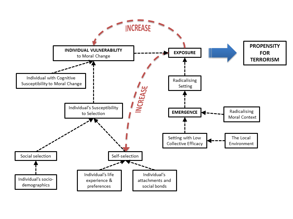
The IVEE framework allows the causal factors across the three levels of the model to interact. The three levels and their interactions can be summarised as a flow chart, as shown in Figure 1. This diagram shows how socio-demographic, cognitive and selective factors contribute to an individual’s overall vulnerability to moral change, and how environmental factors contribute to the emergence of a radicalising setting. When a vulnerable individual becomes exposed to such a setting they develop an increased propensity to commit acts of terrorism. The red arrows indicate parts of the model affected by feedback: increased exposure to radicalising settings increases the self-selective factors contributing to an individual’s vulnerability to moral change, and also increases that vulnerability directly.
Adapting IVEE into a Simulation
The modelling technique chosen to represent the IVEE theoretical framework is an individual-level state-transition model (STM). STMs are commonly used in epidemiology to describe the spread of infectious diseases, with the simplest version being the basic SIR model (Keeling & Rohani 2008). The SIR model represents the process of infection, where a person can be in one of three states: “susceptible”, “infectious”, or “resistant”. The arrangement of these states is illustrated in Figure 2.

In this diagram the circles represent states and the boxes represent transitions between the different states. Every transition has an equal number of inputs and outputs, so in the process of “infection” a susceptible person becomes exposed to an infected person, and the output of that process is two infected people. The process of “recovery” is simpler, just requiring one infectious person as input and one recovered person as output.
The state-transition example in Figure 2 uses only one type of agent — a person — which can be in any one of the three different states. However, these models can also be extended to use multiple types of agent. For example, the spread of malaria can be modelled using two types of agent (people and mosquitos) which can each take one of two different states (susceptible / infected for people, and susceptible / carrier for mosquitos). This flexibility makes it an ideal tool for reframing the IVEE model, which describes the process by which two different agents — people and settings — change state from unradicalised to radicalised. We can therefore rewrite the IVEE theoretical framework as a state-transition model with two different types of agent, each with two states, and with two transitions. This is shown in Figure 3.
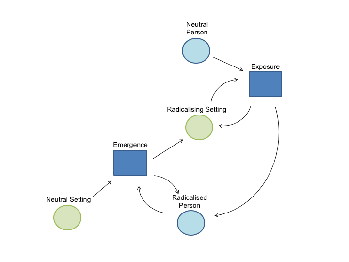
In Figure 3 the transition called “Exposure” causes a Radicalising Setting to have an effect on a Neutral Person to turn them into a Radicalised Person. Similarly, the “Emergence” transition sees a Neutral Setting turn into a Radicalising Setting, through the presence of a Radicalised Person.
In order to turn this theoretical model into a computer simulation we need to define appropriate functions for the two transitions, Exposure and Emergence, and to calibrate them. We therefore need to determine the precise relationships between the causal factors in the IVEE framework. In particular, to define the Exposure Transition we need to know:
- How does a person’s cognitive susceptibility and their exposure to radicalising settings relate to their propensity for terrorism?
- How can we simulate exposure to radicalising moral contexts?
- How is individual cognitive susceptibility distributed in the population and does it change over time?
Similarly, to define the Emergence Transition we need to know:
- What factors make a setting more or less likely to become radicalising?
- What is the relationship between these factors and how radicalising a setting is?
Finally, we need to define:
- What does it mean for a person to be “radicalised” in the model?
We have tried wherever possible to answer these questions using empirical studies, however as already discussed data about the radicalisation process is severely limited. To fully parameterise the model we have thus additionally had to rely on proxies, theoretical hypotheses, common-sense logic, and some trial and error. In order to be explicit about where our assumptions are based on empirical data and where our parameterisation has been less rigorous, we have summarised our sources below:
- How a person’s cognitive susceptibility and exposure to radicalising settings relate to their propensity: we have based this part of the model on an empirical source that relates cognitive susceptibility and exposure to a person’s propensity for general types of crime (Meldrum et al. 2013). No empirical sources were available to extend this to terrorism, so we have used statistics on the prevalence of serious crime, and common-sense logic about the similarities and differences between general crime and terrorism.
- To simulate exposure to radicalising moral contexts: we have drawn a parallel with previous studies on how people decide where to spend their time. The primary source is Harris and Wilson’s 1978 research into the popularity of retail centres, which we have modified using theory from the literature on radicalisation.
- Distribution of individual cognitive susceptibility: we have used empirical studies into the psychology of cognitive susceptibility to build this part of the model. We have drawn on Wikström (2009a) as the basis for this, although to obtain the level of detail required to simulate cognitive susceptibility we used a proxy to represent an individual’s morality. The proxy chosen is Resistance to Peer Influence, developed by Steinberg & Monahan (2007), which has been found in several empirical studies to be linked to delinquency.
- The factors underlying emergence: this is the least well researched part of the IVEE framework, and we have had to rely heavily on theoretical work to define this part of the model. The theoretical research we have relied on for this are the studies about emergence already discussed, namely Wikström & Treiber (2009), Wikström (2011), and Sampson (2004, 2009). Due to the absence of data we have kept this part of the model as simple as possible and calibrated it using trial and error, by checking that the model outputs satisfy a list of stylised facts (discussed further in Section 4.)
- The relationship between the factors underlying emergence: this is even less well understood than the factors themselves, and we have had no data on which to draw. We have therefore chosen a simple relationship based on common-sense logic to build this part of the model.
- Definition of “radicalised”: our definition of what it means to be radicalised in the model flows from the way the rest of the model has been calibrated. The IVEE framework assumes there is no fundamental difference between the process of radicalisation and the process by which propensity for crime more generally develops, but there clearly are differences between terrorism and other crimes, so we have ensured the model is calibrated to describe radicalisation, not criminality development.
We shall now look in detail at how the separate parts of the model were developed.
Defining the exposure transition
Cognitive susceptibility
An individual’s cognitive susceptibility to radicalisation can be determined by their capability to exercise self-control and morality. The literature suggests self-control is largely fixed by the time a child enters kindergarten, so in the model it is assumed to be constant for each person. Wikström (2009a) assumes ability to exercise self-control to be normally distributed across the population, and in the absence of other information so shall we.
However an individual’s morality cannot be assumed to be constant. Large-scale longitudinal neurological studies into morality have not been conducted, so to determine an appropriate distribution for morality we shall have to use a proxy. A reasonable proxy for this is a self-report measure called Resistance to Peer Influence (RPI), developed by Steinberg & Monahan (2007). It is calculated by presenting individuals with 10 pairs of statements and asking them to choose the statement that describes them best – for example “some people go along with their friends just to keep them happy” versus “other people refuse to go along with what their friends want to do, even though they know it will make their friends unhappy”. This measure has been used in several large studies that have observed its statistical significance as a predictor of delinquent behaviour (Steinberg & Monahan 2007; Monahan et al. 2009; Meldrum et al. 2013), and is supported by older research into the effects of susceptibility to peer pressure on criminal propensity (Erickson et al. 2000).
To use RPI as a proxy for morality in the simulation we need to determine the distribution of RPI in the general population, and to identify any relationships with individual attributes such as age or gender. Meldrum et al. (2013)’s study found RPI to be approximately normally distributed, while Steinberg & Monahan (2007)’s study calculated a mean and a variance. All studies using RPI have observed that it varies with age over the period of middle adolescence, with Steinberg and Monahan identifying a linear trend over the ages 14 to 18. This trend is the same for both males and females, but findings have shown females have higher RPI than males. This finding is supported by prior research showing girls generally to be less susceptible to peer pressure than boys (Berndt 1979; Greenberger 1982; Steinberg & Silverberg 1986).
Simulating exposure
As previously discussed, for a person to be exposed to a radicalising moral context there are two requirements: a setting needs to have developed a radicalising moral context, and a person needs to go there. We therefore need to simulate how radicalising a setting is and how long a person spends in it.
We first consider how to model the length of time a person spends in a setting. We can do this by simulating activity fields for each of the simulated people in the model. A person’s activity field is influenced by social selective and self-selective factors: social selective factors can be incorporated by making assumptions based on socio-demographic information, such as “students spend 40 hours per week at university” or “religious people attend their place of worship for approximately 2 hours per week”, but modelling self-selective factors is more complicated.
To model self-selective factors we need to consider why an individual might be more likely to go to one setting over another. This is impossible to model precisely, as by their very nature self-selective factors are individualistic. However, one logical hypothesis to put forward is that a person is more likely to go to locations where similar people also go – a phenomenon called homophily (Kandel 1978; Kandel et al. 1990). It can also be assumed that individuals are more likely to go to places located closer to where they live or work. Additionally, a place that attracts a larger number of people will attract people from a wider catchment area, so the size of a setting also matters.
The influence of a setting’s size and proximity to a person’s home have been used in previous models of individuals’ movements. In particular, Harris & Wilson (1978) created a model of the popularity of retail centres where they modelled the flow of money from one location to another. While modelling money flows may seem somewhat distant from the concept we are modelling here, Harris and Wilson’s model has formed the basis of other simulations from which we can draw a parallel, such as Davies et al (2013)’s research into the locations in London that attracted rioters in 2013.
Harris and Wilson suggested that a flow of money \(f_{ij}\) from location \(i\) to location \(j\) can be modelled by
| $$f_{ij}=A_iQ_iW_j^a e^{-bc_{ij}}$$ | (1) |
In this equation \(W_j\) is the attractiveness of the setting and relates to its size, \(c_{ij}\) is a measure of the cost of travel from \(i\) to \(j\), \(Q_i\) is the retail demand in location \(i\), which is a measure of how much the people in location \(i\) go out to buy things in general, and \(a\) and \(b\) are model parameters (Harris & Wilson 1978). This equation estimates the likelihood that each person \(i\) visits each setting \(j\). In other words, it provides a means of estimating a person's activity field.
For the equation to work in our model it will be necessary to make certain adjustments. Firstly, as activity fields are for people rather than for settings, we need to define \(i\) to be an individual rather than a setting. Next we need to define what we mean by ``cost'' and ``attractiveness'' for functions \(c\) and \(W\) respectively. A simple way to define cost is as the distance between two locations. For attractiveness we can incorporate the factors that make a person more likely to go to one setting over another – namely its size, and the presence of other like-minded people. This makes \(W\) a function of both \(i\) and \(j\), as its value will vary for each person \(i\) and location \(j\). There are many ways we could define \(W\); we have chosen a simple one, which is to measure size by either the number of people who regularly attend the location or its floorspace, and to multiply this by a ``similarity function'', which considers how similar person \(i\) is to each person who has visited location \(j\) in the last time-step. The attributes of a person featuring in this similarity function are their age, religion, self-control, SPI, and propensity.
Variable \(Q_i\) also needs adjusting to make it transferable to the radicalisation model. In the retail model this variable is the retail demand in location \(i\). The equivalent for our model would be the proportion of time person \(i\) spends at a particular type of location. This enables us to incorporate social selective factors such as whether someone is a student or in full-time employment into the activity field. An extra layer of complexity needs to be added to make this work, which is the introduction of setting types. For example, universities and offices are types of workplace, while churches and mosques are types of religious establishment. We can then say that a simulated person who is a student and a Christian will spend 40 hours per week at a university and 2 hours per week at a church, while a full-time employed Muslim spends 40 hours per week at an office and 2 hours per week at a mosque.
The second aspect of simulating exposure is to model how radicalising a setting is. To do this we again turn to the literature on criminality, and what external factors cause an individual’s own delinquent behaviour to increase. In particular, a number of studies have investigated the influence of peer delinquency on an individual (Brendgen et al 2000; Elliot & Menard 1996; Farrington 2004; Heinze et al 2004; Lipsey & Derzon 1998; Patterson et al 1991). However, the IVEE framework uses the more general idea of “moral contexts”, rather than just peer influence. We therefore need a measure for the level of radicalisation of a setting that incorporates both peer influence and environmental features. Activity fields present a simple way to incorporate peer influence: when a simulated individual regularly goes to the same setting as another individual, the two can be considered affiliates and their respective propensities for terrorism can be made to contribute to each other’s exposure. Incorporating environmental features will be considered when we consider how to model emergence.
It still remains to determine the relationship between cognitive susceptibility, exposure to radicalising settings, and actual radicalisation. Again we can turn to the literature on criminality to find a place to start, by considering the relationship between susceptibility to peer influence (SPI), self-control, peer delinquency, and propensity for delinquency (where we take SPI to be the direct opposite of RPI – that is, it is RPI with the scales reversed).
One study which has explored this relationship is Meldrum et al. (2013), which fitted a regression model using a composite self-report delinquency measure as the dependent variable. Meldrum et al. found that the most suitable statistical model linking SPI, self-control, and peer delinquency to their delinquency measure was a negative binomial regression. In their model the number of different delinquent acts conducted by an individual of age 15 over a 12 month period is assumed to be a random variable \(Y\) such that the probability that a person commits \(y\) delinquent acts in the next 12 months is:
| $$P(Y=y)=\frac{\Gamma(y+\frac{1}{a})}{\Gamma(y+1)\Gamma(\frac{1}{a})}\Biggl(\frac{1}{1+a\mu} \Biggr)^{\frac{1}{a}}\Biggl(\frac{a\mu}{1+a\mu} \Biggr)^{y}$$ | (2) |
The parameters \(a\) and \(\mu\) are calculated from the data via the regression model, with the optimum model produced by Meldrum et al. (2013) setting \(a =\) 0.1228 and
| $$\ln\mu=b_0 + b_1 x_1 + b_2 x_2 + b_12 x_1 x_2 + b_3 x_3 =\\ -0.23 + 0.25x_1 - 0.13 x_2 + 0.15 x_1 x_2 + 0.69 x_3$$ | (3) |
If we can define an individual's criminal propensity in terms of \(Y\) then we can use this relationship to calculate an individual's propensity for crime given their SPI, self-control, and exposure to delinquent peers. For example, we could define criminal propensity to be the probability that an individual commits any crimes at all in the next 12 months. In which case we can write a person's criminal propensity as \(P(Y>0)\). Therefore:
| $$P(Y>0)=1-P(Y=0)=\\1-\Biggl( \frac{1}{1+0.1228e^{-0.23+0.25 x_1 - 0.13 x_2 + 0.15 x_1 x_2 + 0.69 x_3}} \Biggr)^{8.14}$$ | (4) |
This gives an average criminal propensity across the population of
| $$E(p)=1-\Biggl( \frac{1}{1 + 0.1228 e^{-0.23}} \Biggr)^{8.14}=0.5314 $$ | (5) |
We now need to consider how to adjust this equation to make it applicable to radicalisation. As no empirical studies have been carried out replicating the results produced by Meldrum et al. (2013) for terrorism, there is no data on which to draw. However, some common-sense logical changes can be made.
Firstly, a radicalised person is someone with the propensity to commit terrorism, and terrorism is not a normal crime. Crimes associated with terrorism are among the most severe, such as homicide or significant property damage. As such severe crimes are much rarer than more minor crimes, the expected value for an average person’s propensity should be far lower than 0.5314. Moffitt et al. (1989) observed that the rate of conviction for a violent offence in young adult males is between 3% an 6%; when spread across the whole population this number becomes lower still, and then lower again if one considers the probability that the violent offence is committed in a particular 12 month period. A more realistic value might then be 0.001. Assuming the value for the parameter \(a\) remains unchanged, this gives \(b_0 =\).
Two other differences between terrorism and more general types of crime can help us make further logical changes to calibrate \(b_1\), \(b_2\), \(b_{12}\) and \(b_3\) in the regression. One is in the level of morality required for an individual to consider a terrorist act to be a reasonable action to take. To illustrate this, consider a homicide committed on an impulse, such as one linked to domestic violence. This would be regarded as a non-terrorist crime and the driving factor behind it would be lack of self-control. In contrast, terrorist homicide is pre-meditated and requires significant planning. This suggests an individual with the propensity to carry out a terrorist act requires a certain level of morality in order to do so, regardless of their ability to exercise self-control. We therefore conclude that morality must have more influence on radicalisation than self-control does, so \(|b_1|>|b_2|\) and \(|b_1|>|b_{12}|\).
The final difference is that radicalising settings are far rarer than more generally criminogenic settings. This can be replicated in the model by assuming that radicalisation will only happen when a particularly susceptible person becomes exposed to a particularly radicalising setting. To meet this criteria we assume that an individual in the top percentile of cognitive susceptibility must become exposed to a setting in the top 5% of radicalising settings to become more radicalised themselves. This provides the following condition:
| $$b_0 + b_1 (2.3263) + b_2 (-2.3263) + b_{12} (2.3263) (-2.3263) + b_3 (2.5758)\\ \geq -2.0243479 $$ | (6) |
Other logical criteria for the parameters are:
- Susceptibility to peer influence and exposure to radicalised peers increase radicalisation, so \(b_1 >\) 0 and \(b_3 >\) 0
- Self-control reduces radicalisation, so \(b_2 <\) 0
- Susceptibility to peer influence has a stronger effect at higher values of self-control (a finding from Meldrum et al’s original paper), so \(b_{12} >\) 0
The precise values chosen were \(b_0 =\) -6.91, \(b_1 =\) 0.9, \(b_2 =\) -0.45, \(b_{12} =\) 0.05 and \(b_3 =\) 0.028, which were found to generate plausible levels of radicalisation in the simulation following some trial and error.
We can now define the exposure transition in the simulation. Following exposure, the propensity \(p\) of person \(i\) to commit an act of terrorism at time \(t\) is:
| $$p_i(t)=1-\Biggl( \frac{1}{1+0.1228e^{-6.91+0.9x_1 -0.45x_2 +0.05x_1 x_2 + 0.028 x_3}} \Biggr)^{8.14} $$ | (7) |
Defining the emergence transition
We have already discussed the hypothesis that settings with low collective efficacy are more likely to become radicalising. The question is how to incorporate the effects of low collective efficacy in the computer simulation in the absence of empirical research. We shall keep our assumptions as simple as possible for this while ensuring the relationships are consistent with the theory laid out in the IVEE framework.
First, we define a collective efficacy coefficient w for each setting, assumed to be constant over time and with 1 as the default value. There are then two mechanisms through which low collective efficacy could cause a setting to become radicalising: radicalised people could be attracted by low collective efficacy, or low collective efficacy could enhance the effect that radicalised people have when they are present – for instance, they could be more influential when at that setting. A setting with a higher number of radicalised people present will then automatically attract more, due to homophily being incorporated into the way activity fields are generated.
A simple way to incorporate the enhanced impact of radicalised people when at settings with low collective efficacy is to multiply the average propensity of the people visiting the setting by \(1/w\). However, following some trial and error in the simulation with different multipliers it was found that multiplying by \(1/\sqrt{w}\) produced more realistic results. (The trial and error process is discussed further in Section 4.
We also need to determine which people should be included when calculating the average propensity of people visiting a setting. Realistically, one would expect that a person would need to spend a certain length of time in a setting before their propensity has any effect. A person might also need to have a minimum propensity to have any influence. We therefore include a time threshold and a propensity threshold into the emergence transition, with the time threshold set at 1 hour per week, and the propensity threshold set at 0.1\(w\). This latter threshold means that an individual with a 10% or higher probability of committing a very severe crime in the next 12 months would be expected to have some radicalising influence on others at a setting with the default collective efficacy. An individual with a 5% chance of committing a very severe crime would only have a radicalising influence at a setting if it had half the default collective efficacy.
We can now define the emergence transition in the simulation. Following emergence, the radicalisation level \(r\) of setting \(j\) at time \(t\) is:
| $$r_i(t)=\frac{1}{n \sqrt{w_j}}\sum_{\textit{s.t.} f>1 \textit{hr} p>0.1w}p_i(t)$$ | (8) |
Defining “radicalisation” in the model
Finally a threshold needs to be set which defines someone as being ''radicalised'' or ''not radicalised'' based on their propensity. This is very subjective as we are dealing with probabilities rather than certainties. However, the parameter a in the negative binomial model acts as a useful guide. This parameter is the heterogeneity parameter, and \(1/a\) indicates the number of ''failures'' expected before one ''success'', where in this instance a success means committing a severe crime. This suggests that a person has (for our value of a) an average of \(1/a =\) 8.14 opportunities to carry out a severe crime where they do not do so, before they finally do. A propensity of \(a=\) 0.1228 therefore seems a reasonable threshold to define what it means to be ''radicalised'' in the absence of any benchmarks.
Input data
The input to the simulation consists of 500 people whose home locations are evenly distributed across the geography. There is an even split across gender, religion (Christian, Muslim, or none), and occupation (employed, unemployed, or studying). The ages of the people at the start of the simulation are evenly divided between the ages of 14 and 30, with the only constraint being that those aged 16 or below all have the occupation “student”. Self-control is generated randomly from a normal distribution with mean 0 and variance 1. SPI is generated randomly, and independently of self-control, from a normal distribution with variance 1 and mean varying according to age and gender so as to be consistent with the findings of Steinberg & Monahan (2007). In order to force the model to begin the process of exposure and emergence, one individual in the model is modified to give them an artificially high value for SPI; this avoided the need to have hundreds of thousands of people in the model before a sufficiently cognitively susceptible person appeared.
The simulation must also be given a location in which to operate to enable the activity fields of the simulated people to be calculated. As the simulated people in the model are fictitious, the environment can also be fictitious. However, as the environment plays an important part in the process it is preferable for there to be elements of realism – for instance by having people’s homes, workplaces and leisure destinations geographically distributed in a way reminiscent of an actual town. This is best achieved by basing the simulated geography on a real location.
The location chosen to provide the basis for the environment to be used in the model is Peterborough, a settlement with a population of approximately 115,000 that has considerable ethnic and social diversity (Wikström et al. 2010). Peterborough is the logical choice for the model’s environment as much of the UK-based research on which the model draws was conducted as part of the Peterborough Adolescent and Young Adult Development Study (PADS+) project.
The environmental attributes of settings which are required inputs in the simulation are the type of setting (workplace, religious establishment, social centres, and residences), the precise location of the settings, the size of the setting, and the collective efficacy of the setting. These first three attributes can be easily estimated for key locations in Peterborough using publicly available data found via a web search. Collective efficacy is more difficult as it would require a large survey to be carried out. However, as precise values are not necessary for the illustration of the simulation, the collective efficacy values for the setting in the model are controlled by the modeller. All are set to 1 by default, except schools and offices which are assumed to have higher collective efficacy, and have been set to 1.25 and 1.67 respectively.
One time-step in the simulation is defined to be one week. The SPI of individuals aged between 14 and 18 reduces every time-step in accordance with the findings of Steinberg & Monahan (2007). \(Q_{ik}\) also changes with time for certain locations, to ensure that as people age they move from schools to universities, and stop visiting youth clubs. The model was run for 260 time-steps, to simulate 5 years. Pseudocode for the full model is in Appendix A.
Model Results
The model was validated using the method of validation against stylised facts. The following stylised facts were derived from the literature on radicalisation, and were used for this purpose:
- The agents in the model should be heterogeneous with regard to radicalism (i.e. the people in the model should not all have the same propensity for terrorism).
- The distribution of propensities for terrorism across the population should be strongly positively skewed (i.e. a very small proportion of people should have any propensity for terrorism whatsoever).
- An individual’s propensity for terrorism can increase or decrease over time.
- A steady state for the system overall should not be reached (i.e. individual propensities can continue to change throughout).
- Radicalising moral contexts (settings) should be extremely rare.
This section shows how the model as calibrated in this article fares against these stylised facts, and considers the drivers behind the observed model behaviour. The interested reader is referred to Pepys (2016) for further sensitivity tests and results of alternative model calibrations.
Heterogeneity of agents
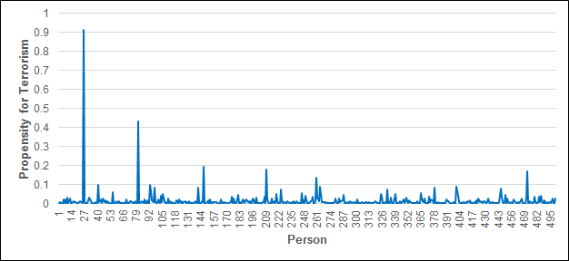
Figure 4 shows the propensities for terrorism of the 500 individuals in the model at the end of the simulation. From this graph it is clear that the agents have different propensities for terrorism, so this stylised fact has been successfully replicated. This behaviour follows logically from the inputs to the exposure transition: \(x_1\) and \(x_2\) in equation (7), representing SPI and self-control, are generated randomly from a normal distribution and are thus unique for each individual. So even if the individuals experienced identical levels of exposure to radicalised peers, they would still have different propensities.
Distribution of propensities for terrorism
A histogram showing the distribution of propensities for terrorism is at Figure 5. This histogram is a comparison between the propensity distributions for the radicalisation model and a version of the model that was calibrated for more general types of crime (more details in Pepys 2016).
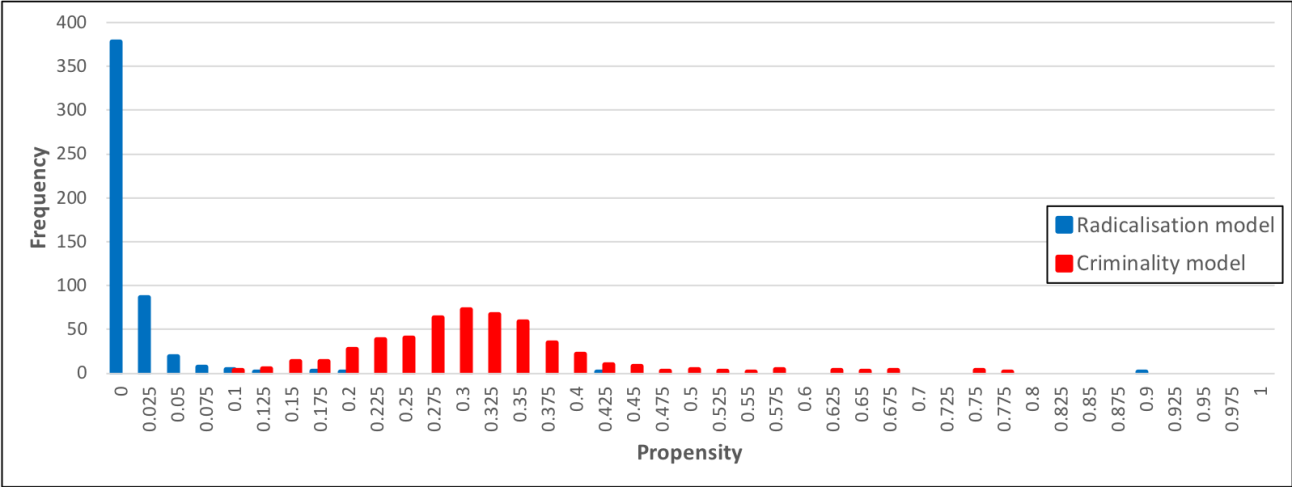
From this histogram it can be seen that there is much less variability in propensities for terrorism than there is for crime in general, with nearly all individuals in the model having extremely low propensity for terrorism. There are a small number of individuals with high propensity for terrorism, but overall there is a strong positive skew. It can therefore be concluded that this stylised fact is satisfied by the model.
The driver behind this behaviour is the value for \(b_0\) in the exposure transition. This parameter has a far greater magnitude than \(b_1\), \(b_2\), \(b_{12}\) or \(b_3\), so the values for \(x_1\), \(x_2\) and \(x_3\) would need to be very large to increase an individual's propensity significantly above 0.001. While the equation may seem odd mathematically, it does produce the desired effect in satisfying this stylised fact.
Change in propensity for terrorism
The graph at Figure 6 shows the propensity for terrorism over time of a random 10 individuals in the model. From this graph it is clear that the propensities of all individuals in the model can both increase and decrease. This follows because each individual’s exposure to radicalised peers also increases or decreases as a result of their activity fields changing over time.
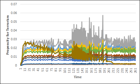
Lack of steady state
Figure 6 also shows that no steady state is reached in the radicalisation model, and that individual propensities continue to change at the end of the simulation. Again this comes from the changes in each individual’s activity field over time. These changes can occur as “forced” changes, such as an individual no longer attending youth groups after they turn 20, or as “organic” changes where they start attending a different setting because it has become more attractive to them. This would happen when more people similar to them also attend the setting. For a steady state to occur the activity fields would need to be kept static, which the model prevents by forcing certain changes as specific ages.
Rarity of radicalising settings
Table 1 shows the distribution of radicalisation levels across public settings (so not including the simulated individual’s homes) at the end of the simulation, compared with the equivalent for the version of the simulation calibrated for general crime.
| Radicalisation/Criminogenity level | Radicalisation model | Criminality model |
| 0 | 42 | 24 |
| 0 to 0.1 | 0 | 13 |
| 0.1 to 0.2 | 5 | 16 |
| 0.2 to 0.3 | 3 | 0 |
| 0.3 to 0.4 | 2 | 2 |
| 0.4 to 0.5 | 0 | 0 |
| 0.5 to 0.6 | 3 | 0 |
| Total | 55 | 55 |
The table shows that for the radicalisation model 42 out of the 55 non-residential settings have zero radicalising influence, while only 24 out of the 55 settings have zero criminogenic influence in the criminality model. The radicalisation model therefore does satisfy this stylised fact. However, it should be noted that there are very few settings that have greater than 0.2 criminogenic influence, while 8 of the 55 setting have greater than 0.2 radicalising influence. This suggests that where radicalising settings do exist they are more likely to be highly radicalising, while criminogenic settings tend to be only weakly criminogenic. Further research would be needed to determine whether this finding is true in the real world.
When calibrating the model this stylised fact was the most difficult to satisfy. It was through ensuring that this stylised fact was satisfied that the value \(b_3\) and multiplier \(1/ \sqrt{w}\) in the emergence transition were determined. For example, Figure 7 shows the distribution of radicalisation levels across settings when alternative multipliers were tried. Some multipliers generated no settings with high enough radicalisation levels to influence the people in the model, while others produce unrealistically high numbers of radicalising settings. The multiplier \(1/ \sqrt{w}\) generated the distribution most aligned to this stylised fact.
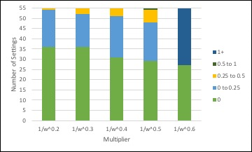
This analysis suggests the model is quite sensitive to changes in these parameters. Further research on collective efficacy and radicalising settings would be required to assess the calibration and improve this part of the model.
Applying the Model to Interventions
The model described in this paper is sufficiently flexible to incorporate counter-radicalisation interventions. Such interventions can target many different mechanisms in the radicalisation process, for example:
- Promotion of a counter-narrative. This takes the form of an organisation (for instance a Government department or specialist charity) distributing media such as audio-visual messaging. The media is designed to strengthen individuals’ knowledge and their ability to think critically, making them less easily influenced and less likely to become exposed to radicalising influences. These counter-narratives could be distributed to the whole population, or just specific at-risk communities.
- Both distribution methods target the same mechanisms in the radicalisation process, but we would expect a targeted campaign to have a greater effect on a smaller number of people.
- Youth groups set up to encourage social cohesion. An example is the Active Change Foundation in East London, whose youth club brings together local young people from an array of ethnic communities, arranges group activities and invites in guest speakers. These groups target self-selection by encouraging young people to be in a setting with high collective efficacy, and they promote critical thinking to make the attendees less susceptible to radicalising influences.
- Targeted one-on-one intervention on a high-risk individual. These interventions are Government-sponsored and can include mentoring, theological guidance, and cognitive behavioural therapy (HMG 2012). If successful we would expect this intervention to significantly reduce an individual’s susceptibility to peer influence and the likelihood they visit radicalising settings in the future.
Interventions such as these can be easily added to the model:
- Universal counter-narrative campaign: where a setting has a radicalisation level above 0.8, multiply the attractiveness factor W by 0.75. Reduce the SPI of all people in the model by 0.1.
- Targeted counter-narrative campaign: at a specific time in the model, reduce the SPI of all people attending a specific setting by 0.5. For these people multiply by 0.6 the attractiveness factor W of settings with radicalisation level above 0.6.
- Targeted intervention against an individual: for any individual with propensity for terrorism above 0.8, over a period of 26 time-steps reduce their SPI by 0.001 each time-step, and multiply by 0.75 the attractiveness factor W of settings with radicalisation level above 0.6.
- Encouraging social cohesion through youth groups: one youth club is given a collective efficacy coefficient of 0.6, and for this setting the attractiveness factor W is multiplied by 1.2 for all people. Individuals spending more than 2 hours at this youth club have their SPI reduced by 0.001 each time-step.
The effects of these interventions can be measured in several ways, such as by comparing the average propensity for terrorism of all people in the model, the maximum propensity for terrorism of any people in the model, or the number of people considered to be “radicalised”. For example, when the interventions above were added to the model the results were as follows:
| Intervention | Mean propensity at t=260 | Max propensity at t=260 | Number radicalised at t=260 |
| No intervention | 0.0169 | 0.9491 | 6 |
| Universal counter-narrative | 0.0121 | 0.8724 | 5 |
| Targeted counter-narrative | 0.0136 | 0.9048 | 5 |
| Targeted individual intervention | 0.0130 | 0.8184 | 5 |
| Youth group | 0.0153 | 0.9290 | 6 |
| All interventions combined | 0.0016 | 0.0318 | 0 |
The effect of the interventions on individuals can vary significantly, since some interventions will have a direct effect on an individual while others an indirect effect. For example, Table 2 shows that the youth group intervention has the smallest overall effect, but for some individuals this intervention has the greatest effect, as shown in Table 3.
| Intervention | Most effective intervention | Least effective intervention |
| Universal counter-narrative | 468 | 0 |
| Targeted counter-narrative | 8 | 63 |
| Targeted individual intervention | 3 | 5 |
| Youth group | 21 | 432 |
This is further illustrated in Figure 8, which displays the reduction in propensity for terrorism of a sample of 8 individuals of different ages following the interventions. If these interventions were implemented differently, for instance if another youth group were chosen, the effects on individuals would change and the intervention could potentially have a greater effect.
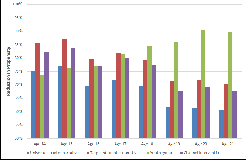
These examples show that in addition to testing whether an intervention has the desired effect, the model can also be used to test how best an intervention could be implemented – for instance which youth group is most effective as a hub for counter-radicalisation activities, or whether it is more effective to use a targeted counter-narrative campaign or a universal one. It can also be used to test for potential unintended consequences, such as an intervention reducing the average propensity of the population in general but not those with the highest propensity.
Interventions designed to reduce crime more generally can also be added, such as by increasing the collective efficacy of settings to model the effect of more visible policing. It is even possible to add the prison system to the model, simply by extending the number of settings and altering the activity fields of those convicted.
Discussion and Conclusions
Strengths of simulation as method
The simulation is based on the IVEE theoretical framework for radicalisation. A valid question is whether the stylised facts could be derived purely from the assumptions behind the IVEE framework, rather than requiring a simulation. This is certainly true for some of the stylised facts: for instance, the heterogeneity of agents follows logically from the individual cognitive susceptibility and susceptibility to selection described by IVEE. Similarly, the lack of steady state and the possibility for propensity to increase or decrease follows from IVEE’s proposal that propensity changes as exposure changes.
However the stylised facts which distinguish between the criminality development and radicalisation processes cannot be explained by IVEE alone. These require additional assumptions, such as those we have made calibrating the simulation. Using simulation as method has highlighted gaps in our knowledge where we have had to rely on using trial and error against stylised facts. It is hoped that by highlighting these knowledge gaps it will encourage further social science research in these areas.
Limitations
This simulation is a considerable simplification of the radicalisation process. This is inevitable, since all models are simplifications of reality, and in the case of radicalisation the process is particularly complex and data is difficult (or impossible) to obtain. Key uncertainties in the model include the way activity fields were generated, the equating of exposure to radicalising moral contexts with exposure to delinquent peers, and the mechanisms behind the emergence of radicalising settings. Several parameters in the model were calibrated through trial and error by seeing whether the resulting model produced plausible results. The model is therefore highly theoretical and in its current state could not be relied upon. Despite this, the model does function, and it provides a starting point upon which to build as further data becomes available and understanding of the radicalisation process grows.
Extension to include virtual settings
The model is sufficiently flexible that it could be adapted to include virtual settings. This would require some modification due to the complexity of the online environment; with the number of websites on the internet now over 1.8 billion (Netcraft 2018), it would be impossible to model each individually. A way around this would be to alter the definition of a setting so that websites with a similar amount of radicalising influence are grouped together as one, and the size of the setting changes as websites of that radicalisation level increase or decrease in popularity. The time people spend online could be modelled as an individual attribute of each person, as could the level of influence they hold. Online radicalisation is a subject of current research interest (see for example Aly et al. 2017; Bastug et al 2018; Whittaker 2018), which would facilitate calibration of the model.
Conclusion
In this paper we have developed a simulation describing the radicalisation process. The radicalisation process is a complex socio-ecological process for which there is very little data, and for this reason at a first glance it does not lend itself to simulation modelling. This paper has argued that despite this, enough data exists to enable a basic model describing the radicalisation process to be created based on the IVEE framework, and this can be used to form the basis of a computer simulation. In order to quantify the causal relationships described in IVEE, such as the processes of exposure and emergence, it has been necessary to draw parallels with the process by which people develop the propensity to commit more general crimes. This has provided a starting point for parameterisation of the simulation. From there we have used logic to determine how the parameters should be calibrated to make the simulation applicable to radicalisation. In so doing we have determined the areas of the process that are least well understood and which would most benefit from further social scientific research.
We have also sought to tackle the difficult problem of how to validate a simulation model when little data exists on the process the simulation is seeking to replicate. We have shown that a method of validation using stylised facts can be formalised to provide a basic level of validation, in that the outputs generated by the simulation developed in this paper do display some realistic features.
The model can be easily adapted to simulate several types of intervention. While the model is not accurate enough to enable the spread of radicalisation to be predicted, it could still be of use for basic comparisons of the effects of different interventions. Ultimately it is only through use of the model and recalibration as more data becomes available that its efficacy can really be explored.
Model Documentation
This model was programmed using C++ and the code is available at: https://www.comses.net/codebases/4d44a66c-5415-4efa-8ffe-81040b4fad82/releases/1.0.0/.Acknowledgements
We acknowledge the support of the Engineering and Physical Sciences Research Council (Grant no: EP/G037264/1).Appendix
Model Initialisation:
- Read in people input file, containing 500 people with the following attributes:
- Initial Age
- Religion (Christian or Muslim, None)
- Occupation (Student, Employed, Unemployed)
- Gender (Male, Female)
- Home location coordinates
- Initial Propensity (all equal to 0.001)
- Read in settings input file, containing 56 settings with the following attributes:
- Name
- Type (School, University, Office, Mosque, Church, High Street, Leisure Centre, Youth Club)
- Location coordinates
- Size (in number of people or floor area)
- Collective Efficacy
- Add people’s home locations to the list of settings (Type: Home)
- Initialise setting attributes:
- Radicalisation level = 0 for all
- Initial average people attributes for all settings (this is used to determine which people are more attracted to which settings):
- Religion = 0.5 (where Christian = 0, Muslim = 1)
- Propensity = 0.5
- Self-Control = 0
- SPI = 0
- Age Group = “19-23”
- Initialise people attributes:
- Self-control generated from N(0, 1) distribution
- SPI generated from \(N(\mu, 1)\) distribution with \(\mu\) varying by age and gender as follows:
| Age | Male | Female |
| 14 or under | 2.0364 | 1.6727 |
| 15 | 1.5382 | 1.1745 |
| 16 | 1.04 | 0.6764 |
| 17 | 0.5418 | 0.1782 |
| 18+ | 0.0436 | -0.32 |
Time-step loop (one time-step represents one week):
- Increase people’s ages and decrease SPI for those aged 14-18
- \(Q_{ik}\), the number of hours person \(i\) spends in settings of type \(k\), using these rules:
- Total hours in a week = 112 (16 waking hours per day)
- If Age < 18, hours at School = 35
- If Age \(\geq\) 18 and Occupation = Student, hours at University = 40
- If Occupation = Employed, hours at Office = 40
- If Religion = Christian, hours at Church = 2
- If Religion = Muslim, hours at Mosque = 2
- If Age < 20, remaining hours divided equally between Home, Friend’s Home, Youth Club, High Street, and Leisure Centre
- If Age \(\geq\) 20, remaining hours divided equally between Home, Friend’s Home, High Street, and Leisure Centre.
- Calculate activity fields for the week as follows:
- Calculate \(D_{ij}\), which defines how different person i is to the average person visiting setting \(j\). \(D_{ij}\) is the average of:
Dreligion : difference between \(i\)'s religion and the average religion of people visiting the setting (where Christian = 0, Muslim = 1)
Dpropensity : difference between \(i\)'s propensity and the average propensity of people visiting the setting
Dage : difference between \(i\)'s age group and the average age group (where "<16" = 0, "16-18" = 1, "19-23" = 2, "24-30" = 3, "31-40" = 4 and "40+" = 5)
Dself-control = \(1 – \exp\{- | i\textit{'s self-control} - \textit{average self-control} | \}\) \(1-\exp\{- | i'\textit{s SPI – average SPI} | \}\).
- Calculate the attractiveness of setting \(j\) to person \(i\) as \(W_{ij} = |j| (1-D_{ij})\), where \(|j|\) denotes the size of setting \(j\).
- Calculate the activity field of person \(i\) as:
- Calculate \(D_{ij}\), which defines how different person i is to the average person visiting setting \(j\). \(D_{ij}\) is the average of:
| Setting type | a | a | ... | k |
| Setting | 1 | 2 | ... | j |
| Time spent (%) | fi1a | fi2a | ... | fijk |
| $$A_{ik}=\frac{1}{\sum_{l\in J_k} W_{il} e^{-c_{ij}}}$$ | (A1) |
- Modify activity fields as follows:
- Ensure people only attend one workplace by setting the workplace generating the largest value of \(f_{ijk}\) to \(Q_{ik}\) and setting all other workplaces to zero.
- Identify each person’s best friend as the person with the activity field most closely resembling their own.
- Ensure the only home visited (other than their own) is that of the best friend, by setting this to \(Q_{ik}\) and setting all other homes to zero.
- Use the activity fields to calculate, for each setting, the mean religion, propensity, self-control, SPI and age group of the people visiting the setting that week. This is used to calculate the following week’s activity fields.
- Use the Emergence function to calculate the radicalisation level of each setting \(j\) as
| $$r_j(t)=\frac{1}{n\sqrt{w_j}} \sum_{i\, \textit{s.t.}\, f>1\, \textit{hr}\, p>0.1w} p_i(t)$$ | (A2) |
- Use the Exposure function to calculate the propensity for terrorism of each person as
| $$p_i(t)=1-\Biggl( \frac{1}{1+0.1228e^{-6.91+0.9x_1-0.45x_2+0.05x_1 x_2 + 0.028x_3 }} \Biggr)^{8.14}$$ | (A3) |
- People output: Person index, Propensity
- Settings output: Setting name, Radicalisation level
References
ALIZADEH, M., C. Cioffi-Revilla, and A. Crooks (2015). The effect of in-group favoritism on the collective behavior of individuals' opinions. Advances in Complex Systems, 18(01n02), 1550002. [doi:10.1142/s0219525915500022]
ALY, A., S. Macdonald, L. Jarvis, and T. M. Chen (2017). Introduction to the special issue: Terrorist online propaganda and radicalization. Studies in Conflict & Terrorism 40 (1), 1-9. [doi:10.1080/1057610x.2016.1157402]
BASTUG, M. F., A. Douai, and D. Akca (2018). Exploring the “Demand Side” of Online Radicalization: Evidence from the Canadian Context. Studies in Conflict & Terrorism, 1-22. [doi:10.1080/1057610x.2018.1494409]
BEAVER, K. M., J. P. Wright, and M. Delisi (2007). Self-control as an executive function: Reformulating Gottfredson and Hirschi’s parental socialization thesis. Criminal Justice and Behavior 34 (10), 1345–1361. [doi:10.1177/0093854807302049]
BERNDT, T. J. (1979). Developmental changes in conformity to peers and parents. Developmental Psychology, 15(6), 608. [doi:10.1037/0012-1649.15.6.608]
BOUHANA, N., P. O. Wikström (2011). Al-Qa’ida-Influenced Radicalisation: A Rapid Evidence Assessment Guided by Situational Action Theory. London: Home Office.
BRENDGEN, M., F. Vitaro, W. M. Bukowski (2000). Deviant friends and early adolescents’ emotional and behavior adjustment. Journal of Research on Adolescence 10, 173–189. [doi:10.1207/sjra1002_3]
CIOFFI-REVILLA, C. (2014). Introduction to computational social science. London and Heidelberg: Springer.
Davies, T. P., Fry, H. M., Wilson, A. G., & Bishop, S. R. (2013). A mathematical model of the London riots and their policing. Scientific Reports, 3, 1303. [doi:10.1038/srep01303]
ELLIOT, D. S. and S. Menard (1996). ‘Delinquent friends and delinquent behavior: Temporal and developmental patterns.’ In J. D. Hawkins (Ed.), Delinquency and crime: Current theories, pp. 28–67. New York: Cambridge University Press.
ELWORTHY, S., G. Rifkind (2006). Making Terrorism History. London: Rider.
ERICKSON, K. G., Crosnoe, R., & Dornbusch, S. M. (2000). A social process model of adolescent deviance: Combining social control and differential association perspectives. Journal of Youth and Adolescence, 29(4), 395-425. [doi:10.1023/a:1005163724952]
FARRINGTON, D. (2004). Conduct disorder, aggression, and delinquency. In R. Lerner and L. Steinberg (Eds.), Handbook of Adolescent Psychology. New York: Wiley. [doi:10.1002/9780471726746.ch20]
FRIEDMAN, N. P., A. Miyake, S. E. Young, J. C. DeFries, R. P. Corley, J. K. Hewitt (2008). Individual differences in executive functions are almost entirely genetic in origin. Journal of Experimental Psychology 137(2), 201–225. [doi:10.1037/0096-3445.137.2.201]
FUMAGALLI, M. and A. Priori (2012). Functional and clinical neuroanatomy of morality. Brain, 135, 2006–2021. [doi:10.1093/brain/awr334]
GALAM, S., M. A. Javarone (2016). Modeling radicalization phenomena in heterogeneous populations. PLoS ONE 11 (5). [doi:10.1371/journal.pone.0155407]
GENKIN, M., A. Gutfraind (2011). How do terrorist cells self-assemble: Insights from an agent-based model of radicalization. Available at SSRN 1031521. [doi:10.2139/ssrn.1031521]
GILBERT, N. and K. G. Troitzsch (1999). Simulation for the Social Scientist. Buckingham: Open University Press.
GREENBERGER, E. (1982). ‘Education and the acquisition of psychosocial maturity.’ In D. McClelland (Ed.), The Development of Social Maturity. New York: Irvington.
HARRIS, B. and A. G. Wilson (1978). Equilibrium values and dynamics of attractiveness terms in production-constrained spatial-interaction models. Environment and Planning 10, 371–388. [doi:10.1068/a100371]
HEINE, B.O., M. Meyer, O. Strangfeld (2005). Stylised facts and the contribution of simulation to the economic analysis of budgeting. Journal of Artificial Societies and Social Simulation 8(4), 4: https://www.jasss.org/8/4/4.html.
HEINZE, H. J., P. A. Toro, K. A. Urberg (2004). Antisocial behavior and affiliation with deviant peers. Journal of Clinical Child and Adolescent Psychology 33, 336–346. [doi:10.1207/s15374424jccp3302_15]
HMG (2012). Channel: Protecting vulnerable people from being drawn into terrorism – A guide for local partnerships. London: Home Office.
KALDOR, N. (1961). ‘Capital accumulation and economic growth.’ In F. A. Lutz and D. C. Hague (Eds.), The Theory of Capital, (pp. 177-222). Palgrave Macmillan, London. [doi:10.1007/978-1-349-08452-4_10]
KANDEL, D. (1978). Homophily, selection, and socialization in adolescent friendships. American Journal of Sociology, 84(2), 427-436. [doi:10.1086/226792]
KANDEL, D., M. Davies, and N. Baydar (1990). ‘The creation of interpersonal contexts: Homophily in dyadic relationships in adolescence and young adulthood.’ In L. Robins and M. Rutter (Eds.), Straight and Devious Pathways from Childhood to Adolescence, pp. 221–241. New York: Cambridge University Press.
KEELING, M. J., P. Rohani (2008). Modeling Infectious Diseases in Humans and Animals. Oxford: Princeton University Press.
KNUTSSON, J. & Tilley, N. (2009). ‘Introduction.’ In J. Knutsson & N. Tilley (Eds.), Evaluating Crime Reduction Initiatives, Volume 24 of Crime Prevention Studies, (pp. 1–6). Monsey, NY: Criminal Justice Press.
LAVER, M. and E. Sergenti (2012). Party Competition: An Agent-based Model. Princeton University Press. [doi:10.23943/princeton/9780691139036.001.0001]
LIPSEY, M. W. and J. H. Derzon (1998). ‘Predictors of violent or serious delinquency in adolescence and early adulthood: A synthesis of longitudinal research.’ In R. Loeber and D. P. Farrington (Eds.), Serious and Violent Juvenile Offenders: Risk Factors and Successful Interventions, pp. 86–105. Thousand Oaks, CA: Sage. [doi:10.4135/9781452243740.n6]
LUM, C., L. W. Kennedy, and A. J. Sherley (2006). The Effectiveness of Counter-Terrorism Strategies. Campbell Systematic Reviews. [doi:10.4073/csr.2006.2]
MELDRUM, R. C., H. V. Miller, J. L. Flexon (2013). Susceptibility to peer influence, self-control, and delinquency. Sociological Inquiry 83(1), 106–129. [doi:10.1111/j.1475-682x.2012.00434.x]
MOFFITT, T. E., S. A. Mednick, and W. F. Gabrielli (1989). Predicting criminal violence: Descriptive data and predispositional factors. In D. Brizer and M. Crowner (Eds.), Current approaches to the prediction of violence, pp. 13–34. Washington D.C.: American Psychiatric Association.
MONAHAN, K. C., L. Steinberg, and E. Cauffman (2009). Affiliation with antisocial peers, susceptibility to peer influence, and antisocial behavior during the transition to adulthood. Developmental Psychology 45(6), 1520–1530. [doi:10.1037/a0017417]
NETCRAFT (2018). January 2018 Web Server Survey. https://news.netcraft.com/archives/2018/01/19/january-2018-web-server-survey.html.
NEUMANN, M. (2015). Grounded Simulation. Journal of Artificial Societies and Social Simulation. 18(1), 9: https://www.jasss.org/18/1/9.html. [doi:10.18564/jasss.2560]
ORMEROD, P. and B. Rosewell (2009). ‘Validation and verification of agent-based models in the social sciences.’ In F. Squazzoni (Ed.), Epistemological Aspects of Computer Simulation in the Social Sciences: Second International Workshop, EPOS 2006, Brescia, Italy, October 5-6, 2006, Revised Selected and Invited Papers, pp. 130–140. Springer Berlin Heidelberg. [doi:10.1007/978-3-642-01109-2_10]
PATTERSON, G. R., D. Capaldi, and L. Bank (1991). ‚An early starter model for predicting delinquency.’ In D. J. Pepler and K. H. Rubin (Eds.), The Development and Treatment of Childhood Aggression, pp. 139–168. Hillsdale, NJ: Erlbaum.
PEPYS, R. C. (2016). Developing Mathematical Models of Complex Social Processes: Radicalisation and Criminality Development. PhD Thesis, University College London.
SAMPSON, R. J. (2004). Neighbourhood and community: Collective efficacy and community safety. New Economy 11, 106–113. [doi:10.1111/j.1468-0041.2004.00346.x]
SAMPSON, R. J. (2009). ‘How does community context matter? Social mechanisms and the explanation of crime rates.’ In P.-O. Wikström and R. J. Sampson (Eds.), The Explanation of Crime: Context, Mechanisms and Development, Chapter 2, pp. 31–60. Cambridge University Press.
SHAFTOE, H., U. Turksen, J. Lever, S. J. Williams (2007). Dealing with terrorist threats through a crime prevention and community safety approach. Crime Prevention and Community Safety 9(4), 291–307. [doi:10.1057/palgrave.cpcs.8150053]
SHAW, C., H. McKay (1942). Juvenile Delinquency and Urban Areas. Chicago: University of Chicago Press.
STEINBERG, L., K. C. Monahan (2007). Age differences in resistance to peer influence. Developmental Psychology 43(6), 1531–1543. [doi:10.1037/0012-1649.43.6.1531]
STEINBERG, L., S. Silverberg (1986). The vicissitudes of autonomy in early adolescence. Child Development 57, 841–851. [doi:10.2307/1130361]
TILLEY, N. (2002). Evaluation for Crime Prevention. Crime Prevention Studies 14. Monsey, NY: Criminal Justice Press.
WHITTAKER, J. (2018). ‘Online Radicalization, The West, and The “Web 2.0”: A Case Study Analysis.’ In Z. Minchev and M. Bogdanoski (Eds.), Countering Terrorist Activities in Cyberspace, pp. 106-120. IOS Press.
WIKSTRÖM, P.O. (2009a). Crime propensity, criminogenic exposure and crime involvement in early to mid-adolescence. Monatsschrift fur Kriminologie und Strafrechtsreform 92, 253–266. [doi:10.1515/mks-2009-922-312]
WIKSTRÖM, P. O. (2009b). ‘Individuals, settings, and acts of crime: situational mechanisms and the explanation of crime.’ In P.-O. Wikström and R. J. Sampson (Eds.), The Explanation of Crime: Context, Mechanisms and Development, pp. 61–107. Cambridge University Press.
WIKSTRÖM, P.O. (2011). ‘Does everything matter? Addressing problems of causation and explanation in the study of crime.’ In J. M. McGloin, C. J. Sullivan, L. W. Kennedy (Eds.), When Crime Appears: The Role of Emergence, pp. 53–72. London: Routledge. [doi:10.4324/9780203802106]
WIKSTRÖM, P.O., V. Ceccato, B. Hardie, K. Treiber (2010). Activity fields and the dynamics of crime. Advancing knowledge about the role of the environment in crime causation. Journal of Quantitative Criminology 26(1), 55–87. [doi:10.1007/s10940-009-9083-9]
WIKSTRÖM, P. O., K. Treiber (2009). ‘What drives persistent offending? The neglected and unexplored role of the social environment.’ In J. Savage (Ed.), The Development of Persistent Criminality. Oxford: OUP. [doi:10.1093/acprof:oso/9780195310313.003.0019]