Simulating Crowds in Real Time with Agent-Based Modelling and a Particle Filter

Introduction

Agent-based modelling is a form of computer simulation that is well suited to modelling human systems (Bonabeau 2002; Farmer & Foley 2009). In recent years it has emerged as an important tool for decision makers who need to base their decisions on the behaviour of crowds of people (Henein & White 2005). Such models, that simulate the behaviour of synthetic individual people, have been proven to be useful as tools to experiment with strategies for humanitarian assistance (Crooks & Wise 2013), emergency evacuations (Ren et al. 2009; Schoenharl & Madey 2011), management of religious festivals (Zainuddin et al. 2009), reducing the risk of crowd stampedes (Helbing et al. 2000), etc. Although many agent-based crowd simulations have been developed, there is a fundamental methodological difficulty that modellers face: there are no established mechanisms for incorporating real-time data into simulations (Lloyd et al. 2016; Wang & Hu 2015; Ward et al. 2016). Models are typically calibrated once, using historical data, and then projected forward in time to make a prediction independently of any new data that might arise. Although this makes them effective at analysing scenarios to create information that can be useful in the design of crowd management policies, it means that they cannot currently be used to simulate real crowd systems in real time. Without knowledge of the current state of a system it is difficult to decide on the most appropriate management plan for emerging situations.

Fortunately, methods do exist to reliably incorporate emerging data into models. Data assimilation is a technique that has been widely used in fields such as meteorology, hydrology and oceanography, and is one of the main reasons that weather forecasts have improved so substantially in recent decades (Kalnay 2003). Broadly, data assimilation refers to a suite of techniques that allow observational data from the real world to be incorporated into models (Lewis et al. 2006). This makes it possible to more accurately represent the current state of the system, and therefore reduce the uncertainty in future predictions.

It is important to note the differences between the data assimilation approach used here and that of typical agent-based parameter estimation / calibration. The field of optimisation — finding suitable estimates for the parameters of algorithms — is an extremely well-researched field that agent-based modellers often draw on. For example, agent-based models regularly make use of sampling methods, such as Latin Hypercube sampling (Thiele et al. 2014) or evolutionary / heuristic optimisation algorithms such as simulated annealing (Pennisi et al. 2008), genetic algorithms, (Heppenstall et al. 2007), and approximate Bayesian computation (Grazzini et al. 2017). There are also new software tools becoming available to support advanced parameter exploration (Ozik et al. 2018).

A fundamental difference between typical parameter optimisation and the data assimilation approach is that data assimilation algorithms aim to estimate the current ‘true’ state of the underlying system at runtime, along with the uncertainty in this estimate, rather than purely trying to find the optimal model parameter values. In other words, data assimilation algorithms adjust the current model state in response to real-time data in order to constrain the model’s continued evolution against observations of the real world (Ward et al. 2016). In contrast, even if optimal model parameters have been found via a standard calibration approach, model stochasticity leads to state estimates whose uncertainty increases over time. Whilst there are some recent studies that attempt to re-calibrate model parameters dynamically during runtime (e.g., Oloo & Wallentin 2017; Oloo et al. 2018), this does not reduce the natural uncertainty in the system state that arises as stochastic models evolve.

This paper is part of a wider programme of work^[1] whose main aim is to develop data assimilation methods that can be used in agent-based modelling. The software codes that underpin the work discussed here are available in full from the project code repository (DUST 2019) and instructions for operating the codes can be found in Section 6. The work here focuses on one particular system, pedestrian movements, and one particular method, the particle filter. A particle filter is a brute force Bayesian state estimation method whose goal is to estimate the ‘true’ state of a system, obtained by combining a model estimate with observational data, using an ensemble of model instances called particles. When observational data become available, the algorithm identifies those model instances, i.e. particles, whose state is closest to that of the observational data, and then re-samples particles based on this distance. It is worth noting that once an accurate estimate of the current state of the system has been calculated, predictions of future states should be much more reliable. Predicting future system states is beyond the scope of this paper however, the focus here is on estimating the current state of the underlying system.

The overall aim of this paper is to:

experiment with the conditions under which a typical particle filter coupled with an agent-based model can estimate the ‘true’ state of an underlying pedestrian system through the combination of a modelled state estimate and observational data.

This will be achieved through a number of experiments following an ‘identical twin’ approach (Wang & Hu 2015). In the identical twin approach, the agent-based model is first executed to produce hypothetical real data — also known as pseudo-truth (Grazzini et al. 2017) data — and these data are assumed to be drawn from the real world. During data assimilation, noisy observations are derived from the pseudo-truth data. This approach has the advantage that the ‘true’ system state can be known precisely, and so the accuracy of the particle filter can be calculated. In reality, the true system state can never be known.

The agent-based model under study is designed to represent an abstract pedestrian system. Rather than developing a comprehensive pedestrian simulation, the model used here is intentionally uncomplicated so that the uncertainty in the evolution of the model can be fully understood. This makes it possible to quantify the conditions under which the particle filter is able to successfully estimate the ‘true’ behaviour of the system. However, the model is sufficiently complex to allow the emergence of crowding, so its dynamics could not be easily replicated by a mathematical model as per Lloyd et al. (2016) and Ward et al. (2016). Crowding occurs because the agents have a variable maximum speed, therefore slower agents hold up faster ones who are behind them. The only uncertainty in the model, which the particle filter is tasked with managing, occurs when a faster agent must make a random choice whether to move round a slower agent to the left or right. Without that uncertain behaviour the model would be deterministic. A more realistic crowd simulation would exhibit much more complicated behavioural dynamics. A further simplification relates to the pseudo-real data that the particle filter uses to estimate the state of the ‘real’ crowd. Currently there is a one-to-one mapping between ‘real’ individuals and agents in the particles. In reality, observational data would be drawn from diverse sources such as population counters, mobile phone cell tower usage statistics, etc., which means that considerable real-time analysis would be required before the data were appropriate for input into the data assimilation algorithm. Hence rather than presenting a proven solution, this paper lays important groundwork towards real-time pedestrian modelling, outlining the considerable challenges that remain.

Background

Agent-based crowd modelling

One of the core strengths of agent-based modelling is its ability to replicate heterogeneous individuals and their behaviours. These individuals can be readily placed within an accurate representation of their physical environment, thus creating a potentially powerful tool for managing complex environments such as urban spaces. Understanding how pedestrians are likely to move around different urban environments is an important policy area. Recent work using agent-based models have shown value in simulating applications from the design of railway stations (Klügl & Rindsfüser 2007; Chen et al. 2017), the organisations of queues (Kim et al. 2013), the dangers of crowding (Helbing et al. 2000) and the management of emergency evacuations (van der Wal et al. 2017).

However, a drawback with all agent-based crowd simulations —aside from a handful of exceptions discussed below — is that they are essentially models of the past. Historical data are used to estimate suitable model parameters and models are evolved forward in time regardless of any new data that might arise. Whilst this approach has value for exploring the dynamics of crowd behaviour, or for general policy or infrastructure planning, it means that models cannot be used to simulate crowd dynamics in real time. The drivers of these systems are complex, hence the models are necessarily probabilistic. This means that a collection of models will rapidly diverge from each other and from the real world even under identical starting conditions. This issue has fostered an emerging interest in the means of better associating models with empirical data from the target system (see, e.g., Wang & Hu 2015; Ward et al. 2016; Long & Hu 2017).

Data-driven agent-based modelling

The concept of Data-Driven Agent-Based Modelling (DDABM) emerged from broader work in data-driven application systems (Darema 2004) that aims to enhance or refine a model at runtime using new data. One of the most well developed models in this domain is the ‘WIPER’ system (Schoenharl & Madey 2011). This uses streaming data from mobile telephone towers to detect crisis events and model pedestrian behaviour. When an event is detected, an ensemble of agent-based models are instantiated from streaming data and then validated in order to estimate which ensemble member most closely captured the particular crisis scenario (Schoenharl & Madey 2008). Although innovative in its use of streaming data, the approach is otherwise consistent with traditional methods for model validation based on historical data (Oloo & Wallentin 2017). Similar attempts have been made to model solar panel adoption (Zhang et al. 2015), rail (Othman et al. 2015) and bus (Kieu et al. 2020) travel, crime (Lloyd et al. 2016), bird flocking (Oloo et al. 2018) and aggregate pedestrian behaviour (Ward et al. 2016), but whilst promising, these models have limitations. For example, they either assume that agent behaviours can be proxied by regression models (Zhang et al. 2015) (which will make it impossible to use more advanced behavioural frameworks to encapsulate the more interesting features of agent behaviour), are calibrated manually (Othman et al. 2015) (which is infeasible in most cases), optimise model parameters dynamically but not the underlying model state (Oloo et al. 2018) (which might have diverged substantially from reality), or use models whose dynamics can be approximated by an aggregate mathematical model (Lloyd et al. 2016; Ward et al. 2016) (neglecting the importance of using agent-based modelling in the first place).

In addition to those outlined above, there are two further studies that are of direct relevance and warrant additional discussion. The first is that of Lueck et al. (2019), who developed an agent-based model of an evacuation coupled with a particle filter. Their aim is to develop a new data association scheme that is able to map from a ‘simple’ data domain, such as that produced by population counters that might exist in the real world, to a more complex domain, such as an agent-based model that aims to simulate the real system. This mapping is important because without such a method it is difficult to determine which observations from the real world should map onto individual agents in the simulation. As with this paper, Lueck et al. (2019) use simulated “ground-truth2 data akin to the 'identical twin' approach. The main difference between this paper and that one relates to the underlying system that is being simulated. Here the agents move across a continuous surface and crowding emerges as the agents collide. In theory the agents can reach any part of the environment, although in practice this is very unlikely because they attempt to move towards specific exits. In Lueck et al. (2019) the agents navigate across a vector road network so their movements are constrained to a set of 100 discrete nodes and there are no collisions or ‘crowding’ as such. Ultimately although the two simulations are drawn from the same research domain, that of pedestrian movements, they are working on different problems. As will be addressed in the discussion, immediate future work for this paper will be to move towards a more realistic pedestrian system and it is expected that the mapping method proposed by Lueck et al. (2019) will be essential as a means of consolidating the aggregate observations that are drawn from the real world with state vector of an agent-based model that simulates individual agents.

The second study is that of Wang & Hu (2015) who investigated the viability of simulating individual movements in an indoor environment using streams of real-time sensor data to perform dynamic state estimation. As with this paper and that of Lueck et al. (2019), the authors used an ‘identical twin’ experimental framework. An ensemble of models were developed to represent the target system with a particle filter used to constrain the models to the hypothetical reality. A new particle resampling method called ‘component set resampling’ was also proposed that is shown to mitigate the particle deprivation problem; see Section 2.10 for more details. The research presented within this paper builds on Wang & Hu (2015) by: (i) attempting to apply data assimilation to a system that exhibits emergence; and (ii) performing more extensive experiments to assess the conditions under which a particle filter is appropriate for assimilating data into agent-based crowd models.

Data assimilation and the particle filter

‘Data assimilation’ refers to a suite of mathematical approaches that are capable of using up-to-date data to adjust the state of a running model, allowing it to more accurately represent the current state of the target system. They have been successfully used in fields such as meteorology, where in recent years 7-day weather forecasts have become more accurate than 5-day forecasts were in the 1990s (Bauer et al. 2015); partly due to improvements in data assimilation techniques (Kalnay 2003). The need for data assimilation was initially born out of data scarcity; numerical weather prediction models typically have two orders of magnitude more degrees of freedom than they do observation data. Initially the problem was addressed using interpolation (e.g., Panofsky 1949; Charney 1951), but this soon proved insufficient (Kalnay 2003). The eventual solution was to use a combination of observational data and the predictions of short-range forecasts (i.e. a model) to create the full initial conditions (the ‘first guess’) for a model of the current system state that could then make forecasts. In effect, the basic premise is that by combining a detailed but uncertain model of the system with sparse but less uncertain data, “all the available information” can be used to estimate the true state of the target system (Talagrand 1991).

A particle filter is only one of many different methods that have been developed to perform data assimilation. Others include the Successive Corrections Method, Optimal Interpolation, 3D-Var, 4D-Var, and various variants of Kalman Filtering; see Carrassi et al. (2018) for a review. The particle filter method is chosen here because it is non-parametric; such methods and are better suited to performing data assimilation in systems that have non-linear and non-Gaussian behaviour (Long & Hu 2017), such as agent-based models. In fact, agent-based models are typically formulated as computer programs rather than in the mathematical forms required of many data assimilation methods, such as the Kalman filter and its variants (Wang & Hu 2015).

The particle filter is a brute force Bayesian state estimation method. The goal is to estimate a posterior distribution, i.e. the probability that the system is in a particular state conditioned on the observed data, using an ensemble of model instances, called particles. Each particle has an associated weight, normalised to sum to one, that are drawn from a prior distribution. In the data assimilation step, discussed shortly, each particle is confronted with observations from the pseudo-real system and weights are adjusted depending on the likelihood that a particle could have produced the observations. Unlike most other data assimilation methods, a particle filter does not actually update the internal states of its particles. Instead, the worst performing particles — those that are least likely to have generated the observations — are removed from subsequent iterations, whereas better performing particles are duplicated. This has the advantage that, when performing data assimilation on an agent-based model, it is not necessary to derive a means of updating unstructured variables. For example, it is not clear how data assimilation approaches that have been designed for mathematical models that consist of purely numerical values will update models that contain agents with categorical variables.

Formally, a particle filter (PF) \(P_k\) consists of an ensemble of simulation realisations and a corresponding set of weights, i.e.

$$P_k = \left\{ (x_k^{(i)}, w_k^{(i)}) : i \in \{1,\dots,N_{\rm p}\} \right\},$$

(1)

where \(N_{\rm p}\) is the number of particles, \(x_k^{(i)}\) is the state vector of the \(i\)-th particle at the \(k\)-th observation, \(w_k^{(i)}\) is the corresponding weight associated with particle \(i\) at observation \(k\), and the weights are subject to the condition \(\sum_{i=1}^{N_{\rm p}} w_k^{(i)} = 1\) for all observations \(k\). The general method of the particle filter is to use \(P_k\), the simulation model and new information in the form of observations to determine \(P_{k+1}\).

There are many different PF methods. The standard form is the sequential importance sampling (SIS) PF which selects the weights using importance sampling (Bergman 1999; Doucet et al. 2000). The particles are sampled from an importance density (Uosaki et al. 2003). One pitfall of the SIS PF is particle degeneracy. This occurs when the weights of all the particles tend to zero except for one particle which has a weight very close to one. This results in the population of particles being a very poor estimate for the posterior distribution. One method to prevent particle degeneracy is to resample the particles, duplicating particles with a high weight and discarding particles with a low weight. The probability of a particle being resampled is proportional to its weight; known as the sequential importance resampling (SIR) PF. The particles can be resampled in a variety of different ways, including multinomial, stratified, residual, systematic, and component set resampling (Liu & Chen 1998; Douc et al. 2005; Wang & Hu 2015). Although resampling helps to increase the spread of particle weights, it is often not sufficient (Carrassi et al. 2018). In a similar manner to particle degeneration in the SIS PF, particle collapse can occur in the SIR PF. This occurs when only one particle is resampled so every particle has the same state.

One of the main drawbacks with PF methods, as many studies have found (e.g., Snyder et al. 2008; Carrassi et al. 2018), is that the number of particles required to prevent particle degeneracy or collapse grows exponentially with the dimensionality of the model. This is an ongoing problem that will be revisited throughout this paper. Hence the work here offers a useful starting point for particle filtering and agent-based crowd modelling, but there are considerable challenges that must be overcome before it can be proven to be useful in a real setting. Fortunately, there are numerous innovations to the particle filter method, which we revisit in Section 5.4, that will help. These include the auxiliary SIR PF and the regularised PF (Arulampalam et al. 2002), the merging PF (Nakano et al. 2007), and the resample-move PF (Gilks & Berzuini 2001), as well as many others (van Leeuwen 2009).

Method

The agent-based model: StationSim

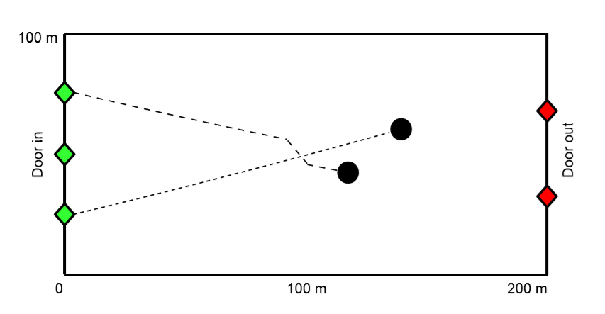
StationSim is an abstract agent-based model that has been designed to very loosely represent the behaviour of a crowd of people moving from an entrance on one side of a rectangular environment to an exit on the other side. This is analogous to a train arriving at a train station and passengers moving across the concourse to leave. A number of agents, N_a, are created when the model starts. They are able to enter the environment, i.e. leave their train, at a uniform rate through one of three entrances. They move across the ‘concourse’ and then leave by one of the two exits. The entrances and exits have a set size, such that only a limited number of agents can pass through them in any given iteration. Once all agents have entered the environment and passed through the concourse then the simulation ends. The model environment is illustrated in Figure 1, with the trajectories of two interacting agents for illustration. All model parameters are specified in Table 1.

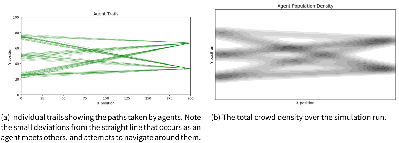
The model has deliberately been designed to be elementary and does not attempt to match the behavioural realism offered by more developed crowd models (Chen et al. 2017; Helbing et al. 2000; Klügl & Rindsfüser 2007; van der Wal et al. 2017). The reason for this simplicity is so that: (1) the model can execute relatively quickly; (2) the probabilistic elements in the model are limited as we know precisely from where probabilistic behaviour arises; and (3) the model can be described fully using a state vector, as discussed in Section 3.7. Importantly, the model is able to capture the emergence of crowding. This occurs because each agent has a different maximum speed that they can travel at. Therefore, when a fast agent approaches a slower one, they attempt to get past by making a random binary choice to move left or right around them. Depending on the agents in the vicinity, this behaviour can start to lead to the formation of crowds. To illustrate this, Figure 2 shows the paths of the agents (2a) and the total agent density (2b) during an example simulation. The degree and location of crowding depends on the random allocation of maximum speeds to agents and their random choice of direction taken to avoid slower agents; these cannot be estimated a priori. Unlike in previous work where the models did not necessarily meet the common criteria that define agent-based models (e.g., Lloyd et al. 2016; Ward et al. 2016) this model respects three of the most important characteristics:

e.g.

• individual heterogeneity — agents have different maximum travel speeds;
• agent interactions — agents are not allowed to occupy the same space so try to move around slower agents who are blocking their path;
• emergence — crowding is an emergent property of the system that arises as a result of the choice of exit that each agent is heading to and their maximum speed.

The model code is relatively short and easy to understand. It is written in Python, and is available in its entirety at in the project repository (DUST 2019). For the interested reader, additional model diagnostics have also been produced to illustrate the locations of collisions, a video of typical model evolution, the total evacuation time, the expected evacuation time were there no collisions, etc^[2].

Data assimilation - Introduction and definitions

DA methods are built on the following assumptions:

1. Although they may have low uncertainty, observational data are often spatio-temporally sparse. Therefore, there are typically insufficient amounts of data to describe the system in detail and a data-driven approach would not work.
2. Models are not sparse; they can represent the target system in great detail and hence fill in the spatio-temporal gaps in observational data by propagating data from observed to unobserved areas (Carrassi et al. 2018). For example, some parts of a building might be more heavily observed than others, so a model that assimilated data from the observed areas might be able to estimate the state of the unobserved areas. However, if the underlying systems are complex, a model will rapidly diverge from the real system in the absence of up to date data (Ward et al. 2016).
3. The combination a model and up-to-date observational data allow "all the available information" to be used to determine the state of the system as accurately as possible (Talagrand 1991).

DA algorithms work by running a model forward in time up to the point that some new observational data become available. This is typically called the predict step. At this point, the algorithm has an estimate of the current system state and its uncertainty; the prior. The next step, update, involves using the new observations, and their uncertainties, to update the current state estimate to create a posterior estimate of the state. As the posterior has combined the best guess of the state from the model and the best guess of the state from the observations, it should be a closer estimate of the true system state than that which could be estimated from the observations or the model in isolation.

The particle filter

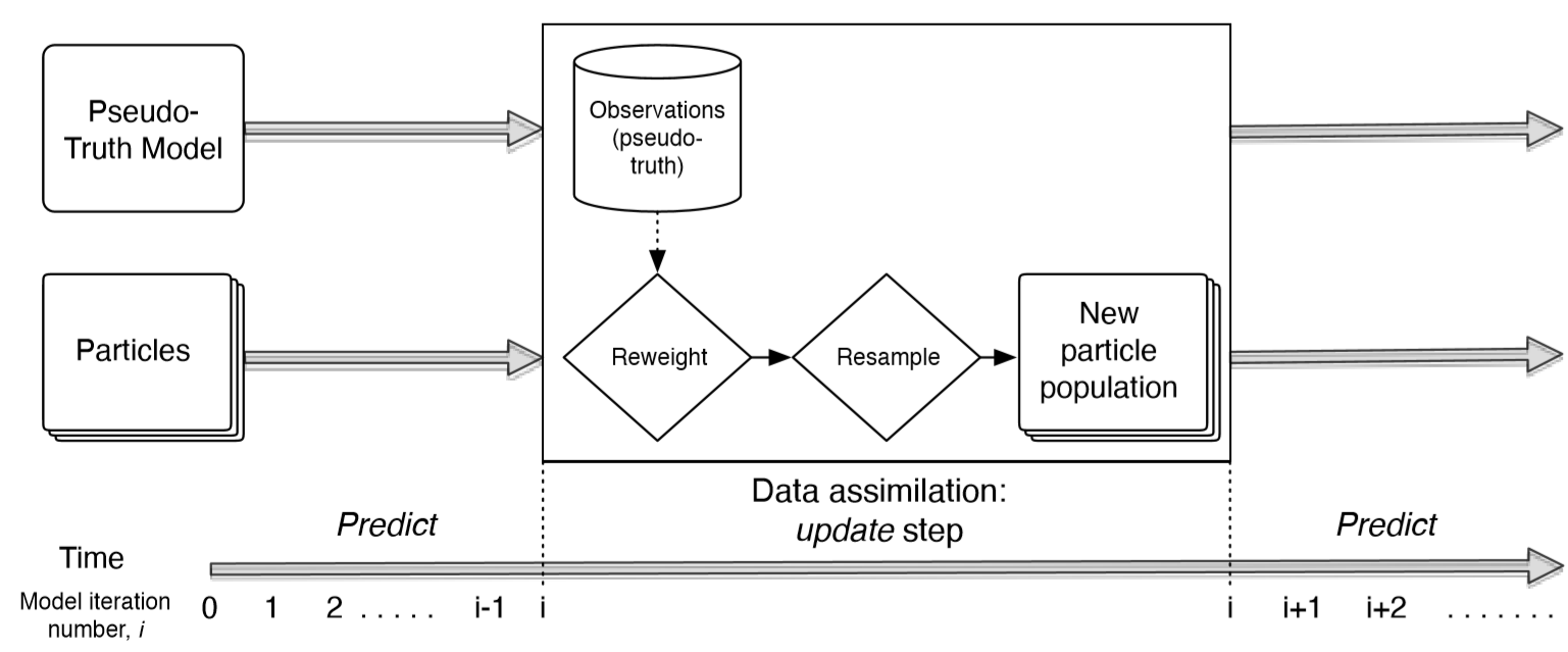
There are many different ways to perform data assimilation, as discussed in Section 2.10. Here, a potentially appropriate solution to the data assimilation problem for agent-based models is the particle filter — also known as a Bayesian bootstrap filter or a sequential Monte Carlo method — which represents the posterior state using a collection of model samples, called particles (Gordon et al. 1993; Carpenter et al. 1999; Wang & Hu 2015; Carrassi et al. 2018). Figure 3 illustrates the process of running a particle filter. Note that the 'pseudo-truth model' is a single instance of the agent-based model that is used as a proxy for the real system as per the identical twin experimental framework that we have adopted. The Sequential Importance Resampling (SIR) filter with systematic resampling is used here because it ranks higher in resampling quality and computational simplicity compared to other resampling methods (Hol et al. 2006; Douc et al. 2005).

The data assimilation ‘window’ determines how often new observations are assimilated into the particle filter. The size of the window is an important factor — larger windows generally result in the particles deviating further from the real system state. Here we fix the window at 100 iterations. We denote the observation times by \(t_k\), for integers \(k\) between 1 and the number of observations \(N_{obs}\), so in the particular case considered here \(t_1\) is the 100th iteration of the simulation, \(t_2\) the 200th etc.

The state vector and transition function

Here, \(x_k^{(i)}\) at time \(t_k\) of the \(i\)-th particle contains all the information that a transition function, i.e. the simulation model, needs to iterate the state forward by one time step, including all agent and simulation environment variables. Here, the particle filter is only used to estimate the model state, but it is worth noting that combined state and parameter estimation is possible (Ward et al. 2016). The state vector for StationSim consists of just the coordinates of each agent, thus \(x_k^{(i)}\in\mathbb{R}^{2N_{\rm a}}\). It is not necessary to store agent velocities since StationSim determines this from each agent’s position and the positions of other agents nearby. Agents’ maximum speeds and exit choices are assumed to be known parameters.

The observation vector \(y_k\) contains all of the observations made from the `real world' (in this case the pseudo-truth model) at the \(k\)-th observation. Here we assume that the observation vector is a measurement of the true state \(x_k\) at time \(t_k\), with the addition of noise, so

$$y_k=x_k+\xi_k$$

(2)

where \(\xi_k\) is uncorrelated Gaussian noise, i.e. \(\xi_k\sim \mathcal{N}(\mathbf{0},\sigma_{\rm m}^2\mathbf{I})\) with mean \(\mathbf{0}\), variance \(\sigma_{\rm m}^2\) and \(\mathbf{I}\) is the \(2N_{\rm a}\) by \(2N_{\rm a}\) identity matrix.

The fact that the state and observation vectors have the same size has the effect of ‘pairing’ agents in each particle to those in the pseudo-truth data, similar to the case considered in Wang & Hu (2015). Consequently, it is worth noting that, because the particle filter will not be tasked with parameter estimation, the data assimilation problem is somewhat less complicated than it would be in a real application where this pairing would not be possible. For example, the agent parameter used to store the location of the exit out of the environment that an agent is moving towards is assumed to be known, consequently the particle filter does not need to estimate where the agents are going, only where they currently are. This is analogous to tracking all individuals in a crowd and providing snapshots of their locations at discrete points in time to the particle filter. This ‘synthetic observation’ is more detailed than data typically available.

Particle weights

Each particle \(i\) in the particle filter has a time varying weight \(w_k^{(i)}\) associated with it that quantifies how similar a particle is to the observations. The weights are calculated at the end of each data assimilation window, i.e. when observations have become available. At the start of the following window the particles then evolve independently from each other (Fearnhead & Künsch 2018). The weights after the \(k\)-th observation are computed as follows. For each particle, the \(l_2\)-norm of the difference between the particle state vector \(x_k^{(i)}\) and the observation vector \(y_k\) is computed,

$$\varepsilon_k^{(i)}=||y_k-x_k^{(i)}||_2,$$

(3)

and the updated weight is then \(w_{k}^{(i)}=\eta/(10^{-9}+\varepsilon_k^{(i)})\), where \(\eta\) is a normalising constant. The mean PF error at the \(k\)-th observation is then

$$\nu_k=\frac{1}{N_{\rm p}}\sum_{i=1}^{N_{\rm p}}\varepsilon_k^{(i)}.$$

(4)

Sampling procedure

Here, a Sequential Importance Resampling (SIR, discussed in Section 2.10) or bootstrap filter is implemented that uses systematic resampling, which is computationally straightforward and has good empiricalperformance (Doucet et al. 2001; Douc et al. 2005; Wang & Hu 2015; Long & Hu 2017; Carrassi et al. 2018). This method requires drawing just one random sample \(U\) from the uniform distribution on the interval \([0,1/N_{\rm p}]\) and then selecting \(N_{\rm p}\) points \(U^i\) for \(i \in \{1,\dots,N_{\rm p}\}\) on the interval \([0,1]\) such that

$$U^i = (i-1)/N_{\rm p} + U.$$

(5)

Using the inversion method, we calculate the cumulative sum of the normalised particle weights \(w_k^{(i)}\) and define the inverse function \(D\) of this cumulative sum, that is:

$$D(u) = i \text{ for } u \in \left(\sum_{j=1}^{i-1}w_k^{(j)},\sum_{j=1}^{i}w_k^{(j)}\right).$$

(6)

Finally, the new locations of the resampled particles are given by \(x_{D(U^i)}\).

Particles with relatively large error, and hence small weight, are likely to be removed during the resampling procedure, whereas those with low error, and hence high weight, are likely to be duplicated. The weighted sum of the particle states,

$$\sum_{i=1}^{N_{\rm p}}w_k^{(i)}x_k^{(i)},$$

(7)

is used to estimate the ‘true’ system state. Other summary statistics can be computed from appropriate weighted sums.

A well-studied issue that particle filters face is that of particle deprivation (Snyder et al. 2008), which refers to the problem of particles converging to a single point such that all particles, but one, vanish (Kong et al. 1994). Here, the problem is addressed in two ways. Firstly, by simply using increasingly larger numbers of particles and, secondly, by diversifying the particles (Vadakkepat & Jing 2006); also known as roughening, jittering, and diffusing (Li et al. 2014; Shephard & Flury 2009; Pantrigo et al. 2005). In each iteration of the model we add Gaussian white noise to the particles’ state vector to increase their variance, which increases particle diversity. This encourages a greater variety of particles to be resampled and therefore makes the algorithm more likely to represent the state of the underlying system. This method is a special case of the resample-move method presented in Gilks & Berzuini (2001). The amount of noise to add is a key hyper-parameter — too little and it has no effect, too much and the state of the particles moves far away from the true state — as discussed in the following section.

Experimental Results

Outline of the experiments

Recall that the aim of this paper is to experiment with the conditions under which a typical particle filter coupled with an agent-based model can estimate the ‘true’ state of an underlying pedestrian system through the combination of a modelled state estimate and observational data. By examining the error— i.e., the difference between the particle filter estimate of the system state and the pseudo-truth data— under different conditions, this paper will present some preliminary estimates of the potential for the use of particle filtering in real-time crowd simulation. In particular, this paper will estimate the minimum number of particles that are needed to model a system that has a given number of agents. The dynamics of the model used here are less complicated than those of more advanced crowd models, and hence the particle filter is tasked with an easier problem than it would have to solve in a real-world scenario. In addition, the number of particles used and the characteristics of the observations provided to the particle filter are much less complicated than would be the case in reality. Therefore, although these experiments provide valuable insight into the general potential of the method for crowd simulation, considerable further work would be required before the method can be used to simulate real crowds in earnest. Sections 5.1 and 5.2 reflect on these factors in detail.

It is well known that one of the main drawbacks with a particle filter is that the number of particles required can explode as the complexity of the system increases (e.g., Snyder et al. 2008; Carrassi et al. 2018). In this system, the complexity of the model is determined by the number of agents. As outlined in Section 3.2, randomness is introduced through agent interactions. Therefore, the fewer the number of agents, the smaller the chance of interactions occurring and the lower the complexity. As the number of agents increases, we find that the number of interactions increases exponentially; Figure 6, discussed in the following section, will illustrate this. This paper will also experiment with the amount of particle noise (\(\sigma_{\rm p}\)) that needs to be included to reduce the problem of particle deprivation, as discussed in Sections 2.2 and 3.12, but this is not a focus of the experiments.

To quantify the 'success' of each parameter configuration — i.e., the number of particles \(N_{\rm p}\) and amount of particle noise \(\sigma_{\rm p}\) that allow the particle filter to reliably represent a system of \(N_{\rm a}\) agents — an estimate of the overall error associated with a particular particle filter configuration is required. There are a number of different ways that this error could be calculated. Here, a three-step approach is adopted. Firstly, the overall error of a single particle is calculated by taking its mean weight after resampling in every data assimilation window. Secondly, to calculate the error associated with all particles in a single experimental result — e.g., a particular \((N_{\rm a}, N_{\rm p})\) combination — the mean error of every particle is calculated. Finally, because the results from an individual experiment will vary slightly, each \((N_{\rm a}, N_{\rm p})\) combination is executed a number of times, \(M\), and the overall error is taken as the median error across all of those individual experiments. The median is chosen because some experiments are outliers, therefore it is a fairer estimate of the overall error across all experiments.

Formally, let \(\nu_k(j)\) be the mean PF error in data assimilation window \(k\) of the \(j\)-th experiment, thus the median of \(M\) experiments of the time-averaged mean PF error is:

$$e_{N_{\rm p},\sigma_{\rm p},N_{\rm a}} = {\rm median}_j \left( \frac{\sum_{k=1}^{N_{\rm obs}}\nu_k(j)}{T} \right)$$

(8)

where \(T\) is the total number of data assimilation windows.

Table 1 outlines the parameters that are used in the experiments. There are a number of other model and particle filter parameters that can vary, but ultimately these do not influence the results outlined here and are not experimented with. The parameters, and code, are available in full from the project repository (DUST 2019).

Table 1: The parameters used in the model and experiments. The Symbol column gives the symbol used to represent the parameter in this paper (where applicable) and Variable gives the variable name in the source code. ‘Experimental’ parameters are varied in the experiments and ‘fixed’ parameters are kept constant throughout all experiments. ‘Secondary’ parameters are important in that they allow crowding to emerge in StationSim, but their values are not of direct relevance to the results of the experiments.

Parameter description	Symbol	Variable	Value/Range
Experimental parameters
Number of agents	\(N_{\rm a}\)	pop_total	\([ 2, 40 ]\)
Number of particles	\(N_{\rm p}\)	number_of_particles	\([ 1, 10000 ]\)
Standard deviation of noise added to particles (drawn from a Gaussian distribution with \(\mu=0\))	\(\sigma_{\rm p}\)	particle_std	\([0.25, 0.5]\)
Fixed parameters
Standard deviation of noise added to observations (drawn from a Gaussian distribution with \(\mu=0\))	\(\sigma_{\rm m}\)	model_std	\(1.0\)
Number of experiments (repetitions)	\(M\)	number_of_runs	20
Model iterations within each data assimilation window	-	resample_window	100
Secondary parameters
Width of the environment	-	width	400
Height of the environment	-	height	200
Number of `in' gates	-	gates_in	3
Number of `out' gates	-	gates_out	2
Minimum distance from a gate that causes pedestrian to leave through that gate	-	gates_space	1
Rate that agents enter the model (the \(\lambda\) parameter in an exponential distribution)	-	gates_speed	1
Minimum agent speed	-	speed_min	0.2
Mean agent speed (individual maximum speeds are drawn from a Gaussian distribution)	-	speed_mean	1
Standard deviation of agent speed	-	speed_std	1
When being blocked by an agent so cannot travel at maximum speed, the number of discrete steps to try as approach the agent to avoid collision	-	speed_steps	3
Minimum distance between agents	-	separation	5
Max distance agents can move when trying to avoid a slower agent	-	max_wiggle	1

Results

Benchmarking

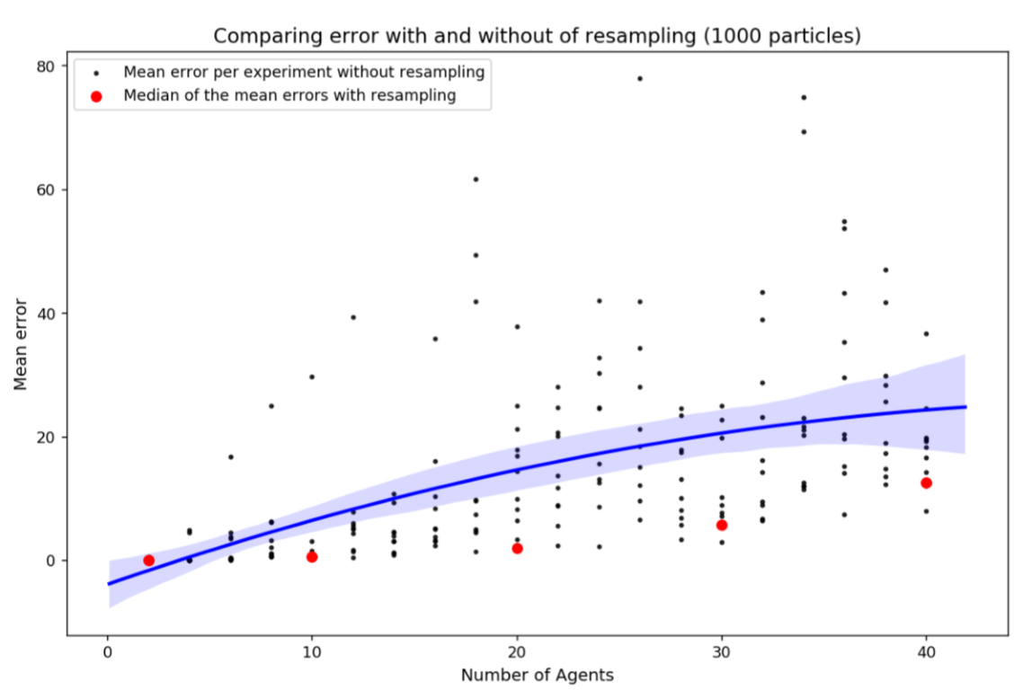
Before experimenting with the particle filter, a set of benchmarking experiments were conducted. In these experiments the particle filter was run as normal but without particle reweighting or resampling. This provides an illustration of the degree of uncertainty that can be attributed to the random interactions of agents in the model and also allows us to quantify the level of error that would be expected were there no data assimilation. The number of agents (\(N_{\rm a}\)) was varied from 2 to 40 in steps of 2 and for each \(N_{\rm a}\) ten individual experiments were conducted. The number of particles chosen does not influence the overall error, so \(N_{\rm p}=1000\) was used in all benchmarking experiments to balance the computational demands of running larger numbers of particles with the drop in consistency that would occur with fewer particles. Figure 4 illustrates the results of the benchmarking experiments. It presents the mean error of the population of particles for each experiment.

The error in Figure 4 increases with the number of agents. This is entirely expected because as the number of agents increases so does the randomness in the model and, hence, the degree to which models will diverge from a pseudo-truth state. Importantly, the red dots illustrate the median error that would be generate with reweighting and resampling (i.e., full data assimilation, discussed in 4.7) under the same numbers of agents and particles. In all cases the error is lower with data assimilation, evidencing the importance of the technique as a means of constraining a stochastic model with some up-to-date observations.

Overall Error

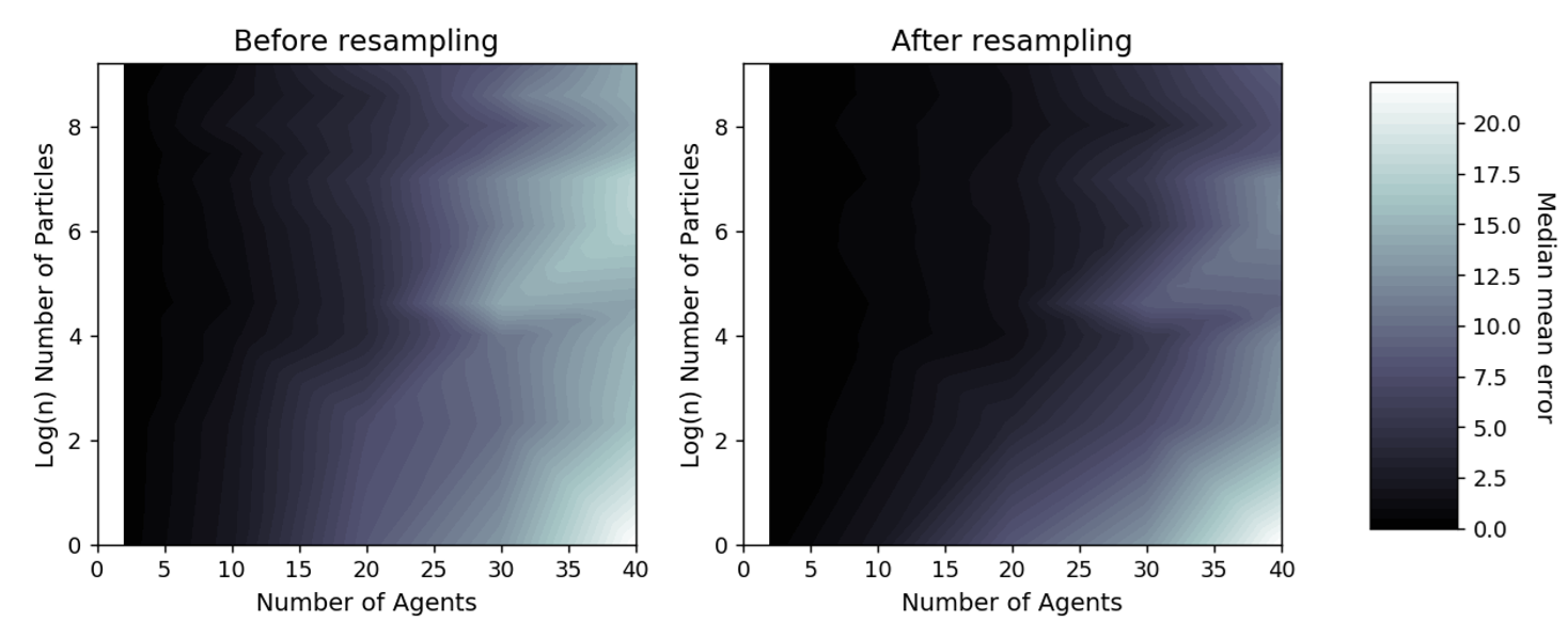
Figure 5 plots the median of the mean error (\(e_{N_{\rm p},\sigma_{\rm p},N_{\rm a}}\) in Equation 8) over all experiments to show how it varies with differing numbers of agents and particles. Due to the computational difficulty in running experiments with large numbers of particles and the need for an exponential increase in the number of particles with the number of agents, discussed in detail below, there are fewer experiments with large numbers of particles and hence the experiments are not distributed evenly across the agents/particles space. Thus, the error is presented in the form of an interpolated heat map. Broadly there is a reduction in error from the bottom-right corner (few particles, many agents) to the top left corner (many particles, few agents). The results illustrate that, as expected, there is a larger error with increasing numbers of agents but this can be mediated with larger numbers of particles. Note the logarithmic scale used on the vertical axis; an exponentially greater number of particles is required for each additional agent included in the simulation.

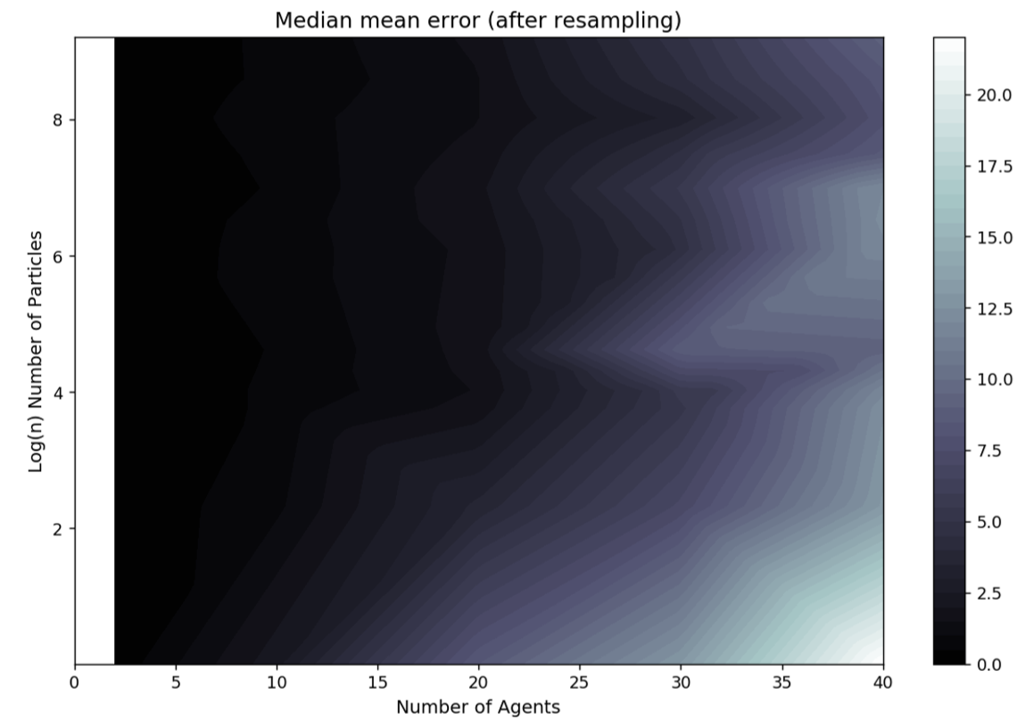
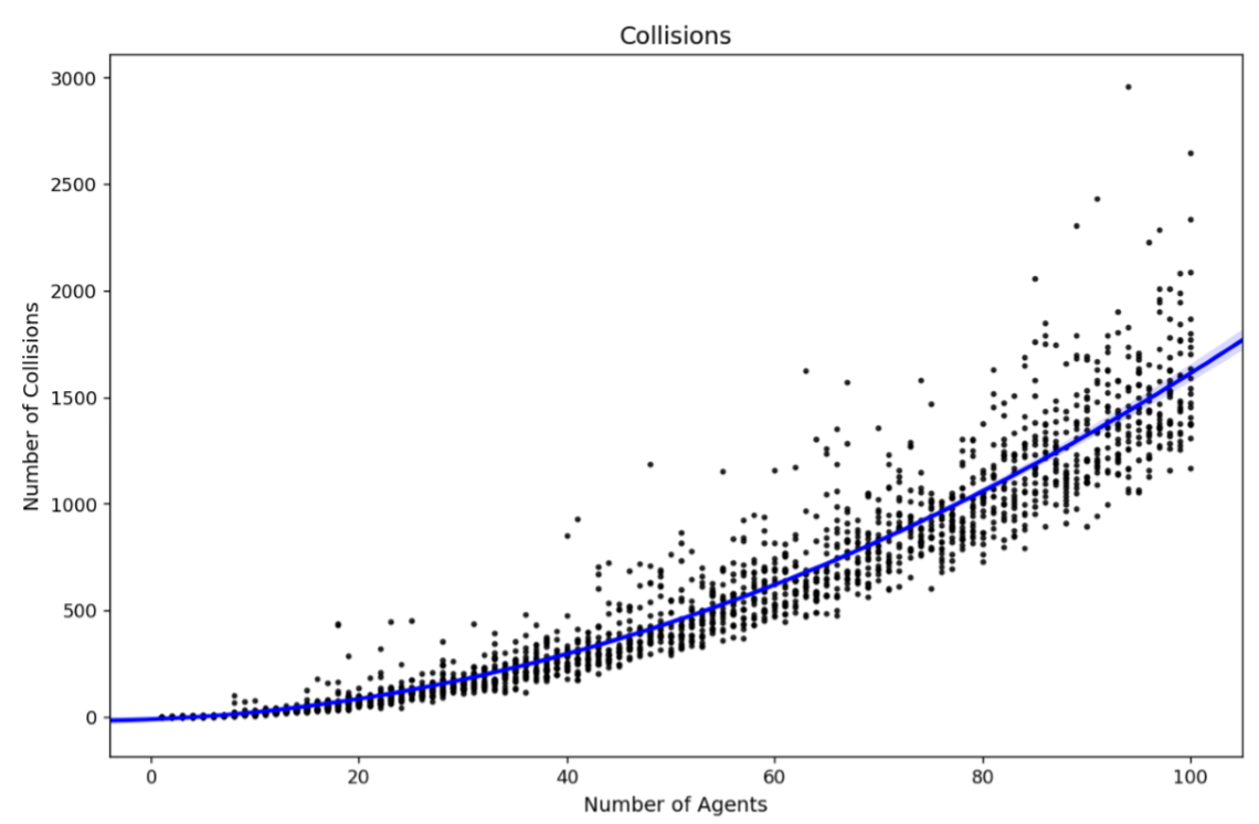
There are two reasons for this exponential increase in the number of particles required. Firstly, as the number of agents increases so does the dimensionality of the state space. Also, with additional agents the chances of collisions, and hence stochastic behaviour, increases exponentially. This is illustrated by Figure 6 which presents the total number of collisions that occur across a number of simulations with a given number of agents.

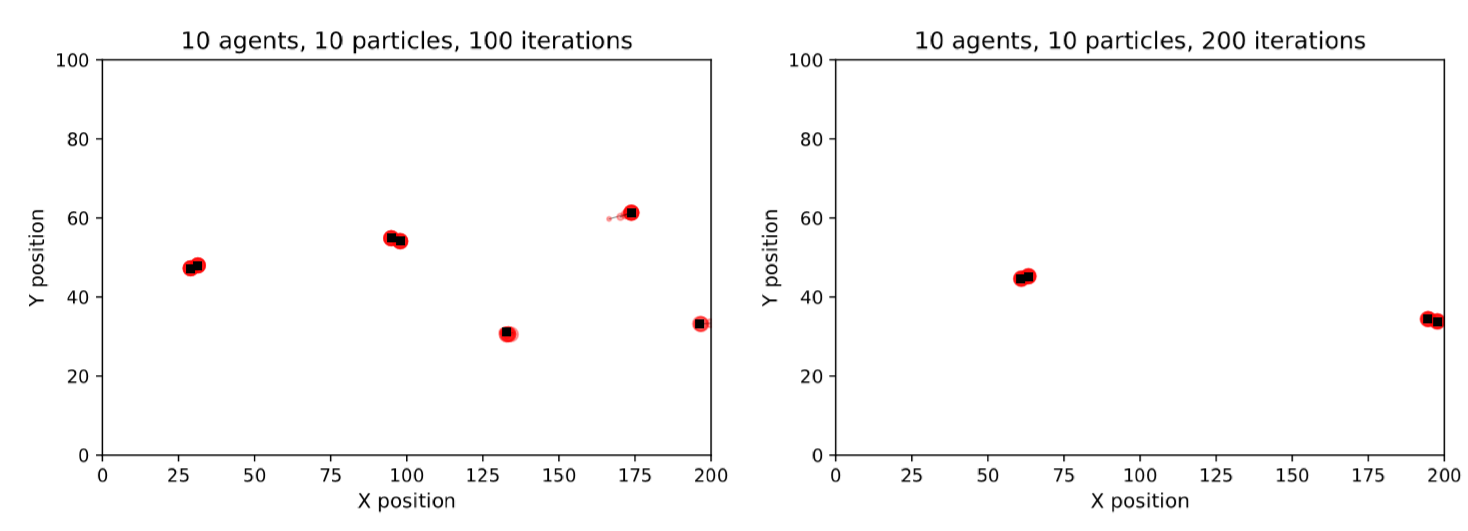
On its own, the overall particle filter error (Figure 5) reveals little information about which configurations would be judged ‘sufficiently reliable’ to be used in practice. Therefore, it is illuminating to visualise some of the results of individual particle filter runs to see how the estimates of the individual agents’ locations vary, and what might be considered an ‘acceptable’ estimate of the true state. Figure 7 illustrates the state of a particle filter with 10 particles and 10 agents at the end of its first data assimilation window (after resampling). With only ten agents in the system there are few, if any, collisions and hence very little stochasticity; all particles are able to represent the locations of the agents accurately.

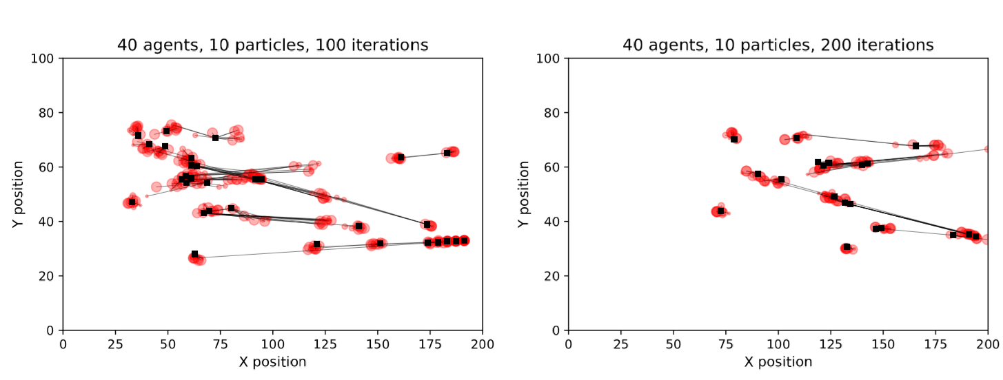
As the number of agents increases, collisions become much more likely and the chance of a particle diverging from the pseudo-truth state increases considerably. It becomes more common that no single particle will correctly capture the behaviours of all agents. Therefore, even after resampling there are some agents whose locations the particle filter is not able to accurately represent. Figure 8 illustrates a filter running with 40 agents and still only 10 particles. The long black lines show the locations of pseudo-real agents and the corresponding agents in the individual particles; it is clear that for some agents none of the particles have captured their pseudo-real locations. This problem can be mediated by increasing the number of particles. Figure 5 showed that with approximately 10,000 particles the error for simulations with 40 agents drops to levels that are comparable to the simulations of 10 agents. Hence a rule of thumb is that any particle filter with an overall error that is comparable to a clearly successful filter, i.e. as per Figure 7, are reliably estimating the state of the system.

Impact of resampling

Resampling is the process of weighting all particles according to how well they represent the pseudo-truth data; those with higher weights are more likely to be sampled and used in the following data assimilation window. This is important to analyse because it is the means by which the particle filter improves the overall quality of its estimates. Figure 9 illustrates the impact of resampling on the error of the particle filter. With fewer than 10 agents in the system resampling is unnecessary because all particles are able to successfully model the state of the system. With more than 10 agents, however, it becomes clear that the population of particles will rapidly diverge from the pseudo-truth system state and resampling is essential for the filter to limit the overall error.

Particle variance

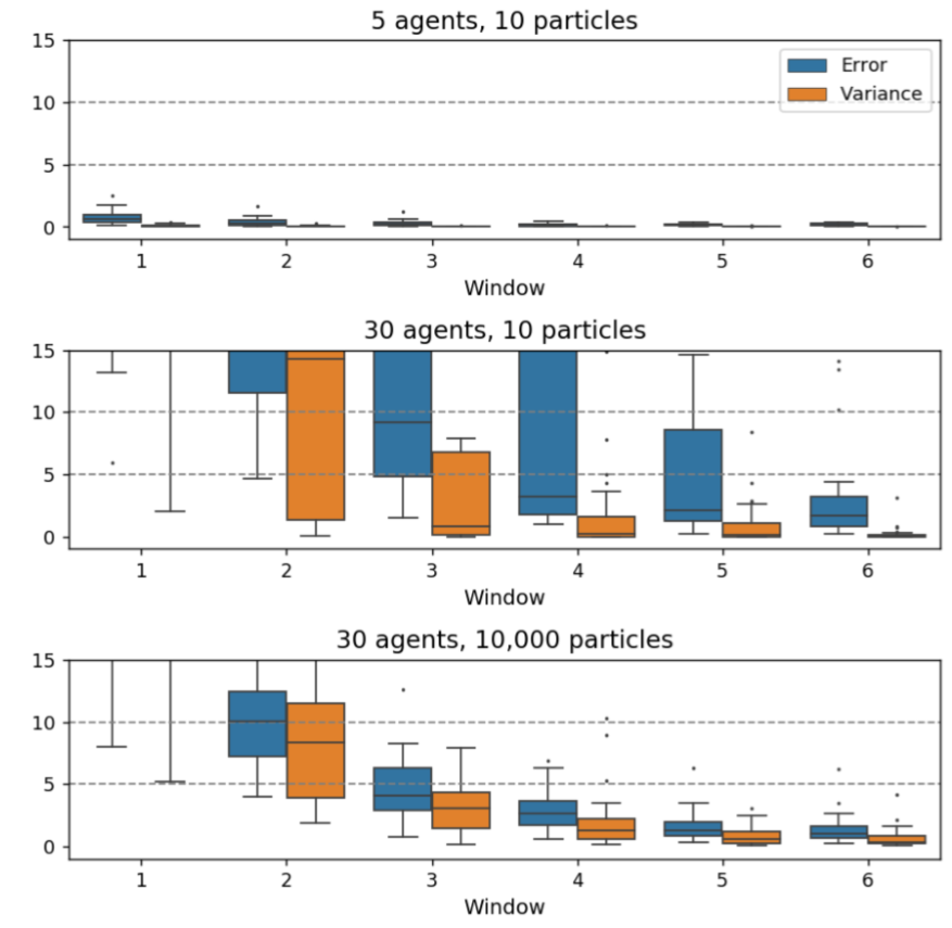
As discussed in Section 3.12, the variance of the population of particles can be a reliable measure for estimating whether particle deprivation is occurring. If there is very little variance in the particles, then it is likely that they have converged close to a single point in the space of possible states. This needs to be avoided because, in such situations, it is extremely unlikely that any particles will reliably represent the state of the real system. Figure 10 illustrates this by visualising the mean error of all particles, νk (defined in Equation 4), in each data assimilation window, k, and their variance under different numbers of agents and particles. Note that each agent/particle configuration is executed 10 times and the results are visualised as boxplots. Also, simulations with larger numbers of agents are likely to run for a larger number of iterations, but the long-running models usually have very few agents in them in later iterations; most have left, leaving only a few slow agents. Hence only errors up to 600 iterations, where most of the agents have left the environment in most of the simulations, are shown. The graphs in Figure 10 can be interpreted as follows:

• With 5 agents and 10 particles there is very low error and low variance (so low that the box plots are difficult to make out on Figure 10). This suggests that particle deprivation is occurring, but there are so few agents that the simulation is largely deterministic so the particles are likely to simulate the pseudo-truth observations accurately regardless.
• When the number of agents is increased to 30 agents and 10 particles, the errors are much larger. The increased non-linearity introduced by the greater number of agents (and hence greater number of collisions) means that the population of particles, as a whole, is not able to simulate the pseudo-truth data. Although particle variance can be high, none of the particles are successfully simulating the target.
• Finally, with 30 agents and 10,000 particles, the errors are relatively low in comparison, especially after the first few data assimilation windows, and a reasonable level of variance is maintained.

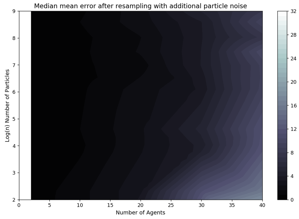
Particle noise

The number of particles (\(N_{\rm p}\)) is the most important hyper-parameter, but the amount of noise added to the particles (\(\sigma_{\rm p}\)) is also important as this is the means by which particle deprivation is prevented. However, the addition of too much noise will push a particle a long way away from the true underlying state. Under these circumstances, although particle deprivation is unlikely none of the particles will be close to the true state. To illustrate this, Figure 11 presents the median error with a greater amount of noise (\(\sigma_{\rm p}=0.5\)). The overall pattern is similar to the equivalent graph produced with \(\sigma_{\rm p}=0.25\) in Figure 5 — as the number of agents in the simulation (\(N_{\rm a}\)) increases so does the number of particles required to maintain low error (\(N_{\rm p}\)) — but the overall error in each \((N_{\rm a}, N_{\rm p})\) combination is substantially larger for the experiments with additional noise. Future work could explore the optimal amount of noise in more detail; \(\sigma_{\rm p}=0.25\) was found to be the most reliable through trial and error.

Discussion and Future Work

Summary

This paper has experimented with the use of a sequential importance resampling (SIR) particle filter (PF) as a means of dynamically incorporating data into an abstract agent-based model of a pedestrian system. The results demonstrate that it is possible to use a particle filter to perform dynamic adjustment of the model. However, they also show that, as expected (Rebeschini & van Handel 2015; Carrassi et al. 2018), as the dimensionality of the system increases, the number of particles required grows exponentially as it becomes less likely that an individual particle will have the ‘correct combination’ of values (Long & Hu 2017). In this work, the dimensionality is proportional to the number of agents. At most 10,000 particles were used, which was sufficient for a simulation with 30-40 agents. However, for a more complex and realistic model containing hundreds or thousands of agents, the number of particles required would grow considerably. In addition, the particle filter used in this study was also provided with more information than would normally be available. For example, information was supplied as fixed parameters on when each agent entered the simulation, their maximum speeds, and their chosen destinations. Therefore, the only information that the particle filter was lacking were the actual locations of the agents and whether they would chose to move left or right to prevent a collision with another agent. It is entirely possible to include the additional agent-level parameters in the state vector, but this would further increase the size of the state space and hence the number of particles required.

These constraints, and the additional computational challenges that would be required to relax them, do not mean that real-time agent-based crowd simulation with a particle filter is not feasible. To begin with, there are many improvements that can be made to this bootstrap filter to reduce the number of particles required. For a thorough review of relevant methods, see van Leeuwen (2009). In addition, it is possible to execute this particle filter on high performance machines with the thousands or tens of thousands of cores to significantly scale up the number of particles. Implementations of particle filters on GPUs are becoming popular (Lopez et al. 2015) due to the huge numbers of GPU cores that can be leveraged to execute the individual particles. The StationSim model would be relatively easy to reimplement in a language that lends itself well to a GPU implementation; current work is exploring this aspect in particular. In addition, although agent-based models are complex, high-dimensional and non-linear, this does not preclude them from successful particle filtering. Geophysical systems, such as the atmosphere or the oceans, are also non-linear and can have state spaces considerably larger than 1 million variables, but have proven amenable to particle filtering (van Leeuwen 2009). Overall, although the experiments here show promise, it is important to note that work is still needed before the aim of simulating a real crowd will be realised.

One particularly encouraging feature of the particle filter is that, unlike other data assimilation approaches, it does not dynamically alter the state of the running model. This could be advantageous because, with agent-based modelling, it is not clear that the state of an agent should be manipulated by an external process. Agents typically have goals and a history, and behavioural rules that rely on those features, so artificially altering an agent’s internal state might disrupt their behaviour making it, at worst, nonsensical. Experiments with alternative, potentially more efficient, algorithms such as 4DVar or the Ensemble Kalman Filter should be conducted to test this.

Improvements to the particle filter

There are a number of possible improvements that could be made to the basic SIR particle filter to reduce the number of particles required. One obvious example is that of Component Set Resampling (Wang & Hu 2015). With that approach, individual components of particles are sampled, rather than whole particles in their entirety. Alternatively, a more commonly used approach is to reduce the dimensionality of the problem in the first place. With spatial agent-based models, such as the one used here, spatial aggregation provides such an opportunity. In the data assimilation stage, the state vector could be converted to an aggregate form, such as a population density surface, and particle filtering could be conducted on the aggregate surface rather than on the individual locations of the agents. After assimilation, the particles could be disaggregated and then run as normal. This will, of course, introduce error because the exact positions of agents in the particles will not be known when disaggregating, but that additional uncertainty might be outweighed by the benefits of a more successful particle filtering overall. In addition, the observations that could be presented to an aggregate particle filter might be much more in line with those that are available in practice; this is discussed in more detail below. If the aim of real-time model optimisation is to give decision makers a general idea about how the system is behaving, then this additional uncertainty might not be problematic. A similar approach, proposed by Rebeschini & van Handel (2015), could be to divide up the space into smaller regions and then apply the algorithm locally to these regions. Although it is not clear how well such a "divide-and-conquer" approach would work in an agent-based model — for example, Long & Hu (2017) developed the method for a discrete cellular automata model — it would be an interesting avenue to explore further.

Towards the incorporation of real-world observations

One assumption made throughout this paper, which limits its direct real-world use, is that the locations of pseudo-real individuals are known, albeit with some uncertainty, and that these locations in the ‘real world’ map directly on to agents in the associated agent-based models that make up the individual particles in the filter. Not only is this mapping unrealistic, it is very unlikely that all individuals in a crowd will be tracked in the first place. Further, we would argue that the privacy implications of tracking individual people are not outweighed by the benefits offered by a better understanding of the system. In reality, the data sources that capture information about pedestrian movements are diverse. They include Wi-Fi sensors that count the number of smart phones in their vicinity (Crols & Malleson 2019; Soundararaj et al. 2020), CCTV cameras that count passers-by (Soldatos & Roukounaki 2017), population density estimates produced using mobile cellular network data (Bogomolov et al. 2014; Grauwin et al. 2015) or social media (McArdle et al. 2012) and occasionally some movement traces of individuals generated from smart-phone applications (Malleson et al. 2018). However, none of the data generated from these sources are going to be directly compatible with the agent-based simulation used to represent reality. In effect, there is a problem of data association; i.e. “determining which observation should be associated with which agent in the simulation” (Lueck et al. 2019). There will need to be processes of aggregation, disaggregation, smoothing, cleaning, noise reduction, etc., in real time in order to map the observation space to the model state space. Fortunately, attempts to create such a mapping are emerging. For example, Lueck et al. (2019) develop a new method that maps anonymous counts of people to individual agents. Similarly, approaches such as that of Georgievska et al. (2019), who estimate overall crowd density from noisy, messy locations of individual smart phones, could be used to combine data from multiple sources but produce a consistent population density surface to inform the data assimilation algorithm. On the whole, however, considerable further work is needed to understand the implications of attempting to assimilate such diverse data into a real-time pedestrian model.

Future work

Ultimately the aim of this work is to develop methods that will allow simulations of human pedestrian systems to be optimised in real time. Not only will such methods provide decision makers with more accurate information about the present, but they could also allow for better predictions of the near future (c.f. Kieu et al. 2020). As discussed previously, there are computational challenges that must be experimented with further, i.e. by leveraging infrastructure that is capable of running millions of particles, and fundamental challenges with regards to mapping real observations on to an agent-based model state space. Both of these areas will be explored by immediate future work. One problem that might arise, particularly with respect to the available data, is whether real observations will be sufficient to identify a 'correct' agent-based model. Therefore, experiments should explore the spatio-temporal resolution of the aggregate data required. Identifiability/equifinality analysis might help initially as a means of estimating whether the available data are sufficient to identify a seemingly ‘correct’ model in the first place. In the end, such research might help to provide evidence to policy makers for the number, and characteristics, of the sensors that would need to be installed to accurately simulate the target system, and how these could be used to maintain the privacy of the people who they are recording.

References

ARULAMPALAM, M. S., Maskell, S., Gordon, N. & Clapp, T. (2002). A tutorial on particle filters for online nonlinear/non-Gaussian Bayesian tracking. IEEE Transactions on Signal Processing, 50(2), 174–188. [doi:10.1109/78.978374]

BAUER, P., Thorpe, A. & Brunet, G. (2015). The quiet revolution of numerical weather prediction. Nature, 525(7567), 47–55. [doi:10.1038/nature14956]

BERGMAN, N. (1999). Recursive Bayesian estimation: Navigation and tracking applications (Doctoral dissertation, Linköping University).

BOGOMOLOV, A., Lepri, B., Staiano, J., Oliver, N., Pianesi, F., & Pentland, A. (2014, November). Once upon a crime: towards crime prediction from demographics and mobile data. In Proceedings of the 16th international conference on multimodal interaction (pp. 427-434). [doi:10.1145/2663204.2663254]

BONABEAU, E. (2002). Agent-based modeling: Methods and techniques for simulating human systems. Proceedings of the national academy of sciences, 99(suppl 3), 7280-7287. [doi:10.1073/pnas.082080899]

CARPENTER, J., Clifford, P. & Fearnhead, P. (1999). Improved particle filter for nonlinear problems. IEE Proceedings - Radar, Sonar and Navigation, 146(1), 2–7. [doi:10.1049/ip-rsn:19990255]

CARRASSI, A., Bocquet, M., Bertino, L. & Evensen, G. (2018). Data assimilation in the geosciences: An overview of methods, issues, and perspectives. Wiley Interdisciplinary Reviews: Climate Change, 9(5), e535. [doi:10.1002/wcc.535]

CHARNEY, J. G. (1951). Dynamic forecasting by numerical process. In Compendium of meteorology (pp. 470-482). American Meteorological Society, Boston, MA. [doi:10.1007/978-1-940033-70-9_40]

CHEN, X., Li, H., Miao, J., Jiang, S. & Jiang, X. (2017). A multiagent-based model for pedestrian simulation in subway stations. Simulation Modelling Practice and Theory, 71, 134–148. [doi:10.1016/j.simpat.2016.12.001]

CROLS, T., & Malleson, N. (2019). Quantifying the ambient population using hourly population footfall data and an agent-based model of daily mobility. Geoinformatica, 23(2), 201-220. [doi:10.1007/s10707-019-00346-1]

CROOKS, A. T. & Wise, S. (2013). GIS and agent-based models for humanitarian assistance. Computers, Environment and Urban Systems, 41, 100–111. [doi:10.1016/j.compenvurbsys.2013.05.003]

DAREMA, F. (2004, June). Dynamic data driven applications systems: A new paradigm for application simulations and measurements. In International Conference on Computational Science (pp. 662-669). Springer, Berlin, Heidelberg. [doi:10.1007/978-3-540-24688-6_86]

DOUC, R., & Cappé, O. (2005, September). Comparison of resampling schemes for particle filtering. In ISPA 2005. Proceedings of the 4th International Symposium on Image and Signal Processing and Analysis, 2005. (pp. 64-69). IEEE. [doi:10.1109/ispa.2005.195385]

DOUCET, A., De Freitas, N., & Gordon, N. (2001). An introduction to sequential Monte Carlo methods. In Sequential Monte Carlo Methods in Practice (pp. 3-14). Springer, New York, NY. [doi:10.1007/978-1-4757-3437-9_1]

DOUCET, A., Godsill, S. & Andrieu, C. (2000). On sequential Monte Carlo sampling methods for Bayesian filtering. Statistics and Computing, 10(3), 197–208. [doi:10.1023/a:1008935410038]

DUST (2019). Data assimilation for agent-based modelling (DUST) project code repository, including StationSim and the particle filter. https://github.com/Urban-Analytics/dust. Accessed: 23/10/2019.

FARMER, J. D. & Foley, D. (2009). The economy needs agent-based modelling. Nature, 460(7256), 685–686. [doi:10.1038/460685a]

FEARNHEAD, P. & Künsch, H. R. (2018). Particle Filters and Data Assimilation. Annual Review of Statistics and Its Application, 5(1), 421–449. [doi:10.1146/annurev-statistics-031017-100232]

GEORGIEVSKA, S., Rutten, P., Amoraal, J., Ranguelova, E., Bakhshi, R., de Vries, B. L., Lees, M. & Klous, S. (2019). Detecting high indoor crowd density with Wi-Fi localization: A statistical mechanics approach. Journal of Big Data, 6(1), 31. [doi:10.31224/osf.io/f7st3]

GILKS, W. R. & Berzuini, C. (2001). Following a moving target-Monte Carlo inference for dynamic Bayesian models. Journal of the Royal Statistical Society: Series B (Statistical Methodology), 63(1), 127–146. [doi:10.1111/1467-9868.00280]

GORDON, N., Salmond, D. & Smith, A. (1993). Novel approach to nonlinear/non-Gaussian Bayesian state estimation. IEE Proceedings F Radar and Signal Processing, 140(2), 107. [doi:10.1049/ip-f-2.1993.0015]

GRAUWIN, S., Sobolevsky, S., Moritz, S., Gódor, I., & Ratti, C. (2015). Towards a comparative science of cities: Using mobile traffic records in New York, London, and Hong Kong. In Computational approaches for urban environments (pp. 363-387). Springer, Cham. [doi:10.1007/978-3-319-11469-9_15]

GRAZZINI, J., Richiardi, M. G. & Tsionas, M. (2017). Bayesian estimation of agent-based models. Journal of Economic Dynamics and Control, 77, 26–47. [doi:10.1016/j.jedc.2017.01.014]

HELBING, D., Farkas, I. & Vicsek, T. (2000). Simulating dynamical features of escape panic. Nature, 407, 487 EP– [doi:10.1038/35035023]

HENEIN, C. M. & White, T. (2005). Agent-Based Modelling of Forces in Crowds. In D. Hutchison, T. Kanade, J. Kittler, J. M. Kleinberg, F. Mattern, J. C. Mitchell, M. Naor, O. Nierstrasz, C. Pandu Rangan, B. Steffen, M. Sudan, D. Terzopoulos, D. Tygar, M. Y. Vardi, G. Weikum, P. Davidsson, B. Logan & K. Takadama (Eds.), Multi-Agent and Multi-Agent-Based Simulation, vol. 3415, (pp. 173–184). Berlin, Heidelberg: Springer. [doi:10.1007/978-3-540-32243-6_14]

HEPPENSTALL, A. J., Evans, A. J., & Birkin, M. H. (2007). Genetic algorithm optimisation of an agent-based model for simulating a retail market. Environment and Planning B: Planning and Design, 34(6), 1051-1070. [doi:10.1068/b32068]

HOL, J. D., Schon, T. B. & Gustafsson, F. (2006, September). On Resampling Algorithms for Particle Filters. In 2006 IEEE Nonlinear Statistical Signal Processing Workshop (pp. 79-82). IEEE. [doi:10.1109/nsspw.2006.4378824]

KALNAY, E. (2003). Atmospheric Modeling, Data Assimilation and Predictability. Cambridge, MA: Cambridge University Press

KIEU, L.-M., Malleson, N. & Heppenstall, A. (2020). Dealing with uncertainty in agent-based models for short-term predictions. Royal Society Open Science, 7(1), 191074. [doi:10.1098/rsos.191074]

KIM, I., Galiza, R. & Ferreira, L. (2013). Modeling pedestrian queuing using micro-simulation. Transportation Research Part A: Policy and Practice, 49, 232–240. [doi:10.1016/j.tra.2013.01.018]

KLÜGL, F. & Rindsfüser, G. (2007). Large-Scale Agent-Based Pedestrian Simulation. In P. Petta, J. P. Müller, M. Klusch & M. Georgeff (Eds.), Multiagent System Technologies, vol. 4687, (pp. 145–156). Berlin, Heidelberg: Springer Berlin Heidelberg. [doi:10.1007/978-3-540-74949-3_13]

KONG, A., Liu, J. S. & Wong, W. H. (1994). Sequential Imputations and Bayesian Missing Data Problems. Journal of the American Statistical Association, 89(425), 278–288. [doi:10.1080/01621459.1994.10476469]

LEWIS, J. M., Lakshmivarahan, S. & Dhall, S. (2006). Dynamic Data Assimilation: A Least Squares Approach. Cambridge, MA: Cambridge University Press [doi:10.1017/cbo9780511526480]

LI, T., Sun, S., Sattar, T. P. & Corchado, J. M. (2014). Fight sample degeneracy and impoverishment in particle filters: A review of intelligent approaches. Expert Systems with Applications, 41(8), 3944–3954. [doi:10.1016/j.eswa.2013.12.031]

LIU, J. S. & Chen, R. (1998). Sequential Monte Carlo Methods for Dynamic Systems. Journal of the American Statistical Association, 93(443), 1032–1044. [doi:10.1080/01621459.1998.10473765]

LLOYD, D. J. B., Santitissadeekorn, N. & Short, M. B. (2016). Exploring data assimilation and forecasting issues for an urban crime model. European Journal of Applied Mathematics, 27(Special Issue 03), 451–478. [doi:10.1017/s0956792515000625]

LONG, Y. & Hu, X. (2017). Spatial Partition-Based Particle Filtering for Data Assimilation in Wildfire Spread Simulation. ACM Transactions on Spatial Algorithms and Systems, 3(2), 1–33. [doi:10.1145/3099471]

LOPEZ, F., Zhang, L., Mok, A. & Beaman, J. (2015). Particle filtering on GPU architectures for manufacturing applications. Computers in Industry, 71, 116–127. [doi:10.1016/j.compind.2015.03.013]

LUECK, J., Rife, J. H., Swarup, S., & Uddin, N. (2019, December). Who goes there? Using an agent-based simulation for tracking population movement. In 2019 Winter Simulation Conference (WSC) (pp. 227-238). IEEE. [doi:10.1109/wsc40007.2019.9004861]

MALLESON, N., Vanky, A., Hashemian, B., Santi, P., Verma, S. K., Courtney, T. K., & Ratti, C. (2018). The characteristics of asymmetric pedestrian behavior: A preliminary study using passive smartphone location data. Transactions in GIS, 22(2), 616-634. [doi:10.1111/tgis.12336]

MCARDLE, G., Lawlor, A., Furey, E., & Pozdnoukhov, A. (2012, August). City-scale traffic simulation from digital footprints. In Proceedings of the ACM SIGKDD International Workshop on Urban Computing (pp. 47-54). [doi:10.1145/2346496.2346505]

NAKANO, S., Ueno, G. & Higuchi, T. (2007). Merging particle filter for sequential data assimilation. Nonlinear Processes in Geophysics, 14(4), 395–408 [doi:10.5194/npg-14-395-2007]

OLOO, F., Safi, K., & Aryal, J. (2018). Predicting migratory corridors of white storks, Ciconia ciconia, to enhance sustainable wind energy planning: a data-driven agent-based model. Sustainability, 10(5), 1470. [doi:10.3390/su10051470]

OLOO, F. & Wallentin, G. (2017). An Adaptive Agent-Based Model of Homing Pigeons: A Genetic Algorithm Approach. ISPRS International Journal of Geo-Information, 6(1), 27. [doi:10.3390/ijgi6010027]

OTHMAN, N. B., Legara, E. F., Selvam, V. & Monterola, C. (2015). A data-driven agent-based model of congestion and scaling dynamics of rapid transit systems. Journal of Computational Science, 10, 338–350. [doi:10.1016/j.jocs.2015.03.006]

OZIK, J., Collier, N. T., Wozniak, J. M., Macal, C. M. & An, G. (2018). Extreme-Scale Dynamic Exploration of a Distributed Agent-Based Model With the EMEWS Framework. IEEE Transactions on Computational Social Systems, 5(3), 884–895. [doi:10.1109/tcss.2018.2859189]

PANOFSKY, R. A. (1949). Objective Weather-Map Analysis. Journal of Meteorology, 6(6), 386–392.

PANTRIGO, J. J., Sánchez, A., Gianikellis, K., & Montemayor, A. S. (2005). Combining particle filter and population-based metaheuristics for visual articulated motion tracking. ELCVIA Electronic Letters on Computer Vision and Image Analysis, 5(3), 68-83. [doi:10.5565/rev/elcvia.107]

PENNISI, M., Catanuto, R., Pappalardo, F. & Motta, S. (2008). Optimal vaccination schedules using simulated annealing. Bioinformatics, 24(15), 1740–1742. [doi:10.1093/bioinformatics/btn260]

REBESCHINI, P. & van Handel, R. (2015). Can local particle filters beat the curse of dimensionality? The Annals of Applied Probability, 25(5), 2809–2866. [doi:10.1214/14-aap1061]

REN, C., Yang, C. & Jin, S. (2009). Agent-Based Modeling and Simulation on Emergency Evacuation. In O. Akan, P. Bellavista, J. Cao, F. Dressler, D. Ferrari, M. Gerla, H. Kobayashi, S. Palazzo, S. Sahni, X. S. Shen, M. Stan, J. Xiaohua, A. Zomaya, G. Coulson & J. Zhou (Eds.), Complex Sciences, vol. 5, (pp. 1451–1461). Berlin, Heidelberg: Springer Berlin Heidelberg [doi:10.1007/978-3-642-02469-6_25]

SCHOENHARL, T. & Madey, G. (2011). Design and Implementation of An Agent-Based Simulation for Emergency Response and Crisis Management. Journal of Algorithms & Computational Technology, 5(4), 601–622. [doi:10.1260/1748-3018.5.4.601]

SCHOENHARL, T. W., & Madey, G. (2008, June). Evaluation of measurement techniques for the validation of agent-based simulations against streaming data. In International Conference on Computational Science (pp. 6-15). Springer, Berlin, Heidelberg. [doi:10.1007/978-3-540-69389-5_3]

SHEPHARD, N., & Flury, T. (2009). Learning and filtering via simulation: Smoothly jittered particle filters. Economics Series Working Papers 469, University of Oxford, Department of Economics.

SNYDER, C., Bengtsson, T., Bickel, P. & Anderson, J. (2008). Obstacles to High-Dimensional Particle Filtering. Monthly Weather Review, 136(12), 4629–4640. [doi:10.1175/2008mwr2529.1]

SOLDATOS, J. & Roukounaki, K. (2017). Development Tools for IoT Analytics Applications. In J. Soldatos (Ed.), Building Blocks for IoT Analytics: Internet-of-Things Analytics, (pp. 81–97). Gistrup, Denmark: River Publishers. [doi:10.13052/rp-9788793519046]

SOUNDARARAJ, B., Cheshire, J. & Longley, P. (2020). Estimating real-time high-street footfall from Wi-Fi probe requests. International Journal of Geographical Information Science, 34(2), 325–343. [doi:10.1080/13658816.2019.1587616]

TALAGRAND, O. (1991). The use of adjoint equations in numerical modelling of the atmospheric circulation. Automatic Differentiation of Algorithms: Theory, Implementation, and Application, 169-180.

THIELE, J. C., Kurth, W. & Grimm, V. (2014). Facilitating Parameter Estimation and Sensitivity Analysis of Agent- Based Models: A Cookbook Using NetLogo and R. Journal of Artificial Societies and Social Simulation, 17(3), 11: https://www.jasss.org/17/3/11.html. [doi:10.18564/jasss.2503]

UOSAKI, K., Kimura, Y., & Hatanaka, T. (2003, December). Nonlinear state estimation by evolution strategies based particle filters. In The 2003 Congress on Evolutionary Computation, 2003. CEC'03. (Vol. 3, pp. 2102-2109). IEEE. [doi:10.1109/cec.2003.1299932]

VADAKKEPAT, P. & Jing, L. (2006). Improved Particle Filter in Sensor Fusion for Tracking Randomly Moving Object. IEEE Transactions on Instrumentation and Measurement, 55(5), 1823–1832. [doi:10.1109/tim.2006.881569]

VAN der Wal, C. N., Formolo, D., Robinson, M. A., Minkov, M. & Bosse, T. (2017). Simulating Crowd Evacuation with Socio-Cultural, Cognitive, and Emotional Elements. In J. Mercik (Ed.), Transactions on Computational Collective Intelligence XXVII, vol. 10480, (pp. 139–177). Cham: Springer International Publishing. [doi:10.1007/978-3-319-70647-4_11]

VAN Leeuwen, P. J. (2009). Particle Filtering in Geophysical Systems. Monthly Weather Review, 137(12), 4089– 4114. [doi:10.1175/2009mwr2835.1]

WANG, M. & Hu, X. (2015). Data assimilation in agent based simulation of smart environments using particle filters. Simulation Modelling Practice and Theory, 56, 36–54. [doi:10.1016/j.simpat.2015.05.001]

WARD, J. A., Evans, A. J. & Malleson, N. S. (2016). Dynamic calibration of agent-based models using data assimilation. Royal Society Open Science, 3(4), 150703. [doi:10.1098/rsos.150703]

ZAINUDDIN, Z., Thinakaran, K. & Abu-Sulyman, I. (2009). Simulating the Circumambulation of the Ka’aba using SimWalk. European Journal of Scientific Research, 38, 454–464

ZHANG, H., Vorobeychik, Y., Letchford, J., & Lakkaraju, K. (2016). Data-driven agent-based modeling, with application to rooftop solar adoption. Autonomous Agents and Multi-Agent Systems, 30(6), 1023-1049. [doi:10.1007/s10458-016-9326-8]