
Introduction
The current financial market involves considerable uncertainty due to the structural complexity of finance and the globalised world. The 2007–2008 financial crisis is one example. The beginning of the crisis was subprime mortgages. However, the fails in subprime mortgages spread widely, and it also affected stock markets. More recently, crashes occurred in the financial market, such as the so-called flash crash. The most famous flash crash was the 2010 Flash Crash, in which stock indices, such as the S&P 500 and Dow Jones Industrial Average, rapidly fell on May 6, 2010. Usually, flash crashes rapidly return to normal patterns. However, sometimes it can cause significant financial disturbances with implications on markets. Moreover, even if market prices after flash crashes are back to normal patterns, these disturbances should be avoided. Since these incidents can lead to financial crises or disruptions, they must be prevented and predicted.
One promising approach is a real-data based approach. This approach is useful for analyzing past incidents but cannot predict future incidents that have never occurred before.
The other promising approach is a numerical-simulation based approach. Especially, agent-based simulation is useful for this kind of research (Edmonds & Bruce 2005). Agent-based simulations aim to imitate the real world by making an imaginary world with agents on computers. Simulations are beneficial because they enable the exploration of hypothetical situations or the prediction of phenomena under certain conditions, such as a new regulation. Especially in financial markets, the importance of agent-based simulation was argued by many scholars (Farmer & Foley 2009; Battiston et al. 2016). For example, Lux & Marchesi (1999) showed that interaction between agents in financial market simulations is necessary to replicate stylized facts in financial markets. Moreover, some simulation models were made based on empirical researches or mathematically validated (Avellaneda & Stoikov 2008; Nagumo et al. 2017). These models can help us to interpret empirical findings of complex systems.
However, these two approaches, i.e., real-data based approach and simulation, are distinct and not sufficiently integrated. Some simulation studies tried to use real data for agent-based simulation. Sajjad et al. (2016) built a demographic movement simulation by using real data. On the other hand, Nonaka et al. (2013) also built an evacuation simulation and used measured data in real evacuation drills. However, in these simulations, real data are used just for setting initial conditions and/or fitting parameters in agent models. In another study targeting financial markets, Braun-Munzinger et al. (2018) built a multi-agent simulation for a bound market. Also, in this study, real data in a bound market was used only for fitting model parameters.
So, in simulations, real data should be used more successfully. If we can do so, simulations can be used with more confidence, and data will offer more than the recorded past. Specifically, financial markets have massive amounts of real data known as tick data. On the other hand, as financial market simulations, computerized virtual markets called artificial markets are present.
In this paper, the real data and simulation results in a financial market are compared as a first step toward an integrated approach. We aimed to find what is missing in the current financial market simulation. In this comparison, we focused on the high-frequency-trader market-making (HFT-MM) strategy. One reason is that HFT agents are influential in the real financial market (Hosaka 2014). The other reason is that the HFT-MM strategy has been well modeled in simulations from previous studies (Avellaneda & Stoikov 2008).
In this paper, first, we quantified the empirical distribution of relative order frequencies of HFT-MM in the real data. Then, we tested whether a simulation model can regrow the same pattern. As a result, we showed that the simulation model partially made the same pattern as the real data. However, there are still differences, which we discussed.
This paper is organized as follows: Section 2.1–2.5 explains the HFT-MM strategy; Section 3.1–3.6 describes previous research; Section 4.1–4.13 shows the data-mining approach used in the behavioral analysis of HFT-MM in the Tokyo Stock Exchange (TSE). Section 5.1–5.20 shows the model and simulation results for HFT-MM in the artificial market we built. In Section 6.1–6.9, we compare the results from our data-mining and simulation analyses. Finally, in Section 7.1–7.7, we discuss the results and conclude with Section 8.1.
What is the HFT-MM Strategy?
In the HFT-MM strategy, traders make many frequent limit orders on the millisecond time scale, made possible through ongoing improvements in information and communication technologies. An MM strategy is specific to limit orders and makes profits by placing buy and sell orders on the order books simultaneously.
Figure 1 shows an example of order books in a continuous double auction. In both the sell and buy order books, there are some orders. Every trader can put their sell or buy orders at any price. (Actually, some regulations on the price range are applied.) In addition, there are two types of orders. One is a “limit order,” or an order with a price. The other is a “market order,” or an order without any price, which means that the traders want to buy or sell shares at any price. Market orders are always executed immediately with the best-priced opposite orders. Usually, limit orders are placed and appear on either the buy or sell order book, hence the term “making” orders. Market orders, conversely, do not appear in the order books and make opposite orders disappear, hence the term “taking” orders.
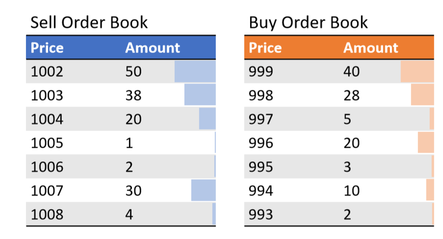
An MM strategy typically uses only making orders, i.e., limit orders, because it aims to realize the profit between the best sell and buy prices and must wait for better conditions by placing orders at a price near the best price. In the case of Figure 1, the MM strategy places sell orders at $1002 and buy orders at $999. After both orders have been executed, the traders receive $3 in profit, i.e., the same as the spread.
However, the MM strategy is always exposed to the risk of price changes. If MM traders have some shares during the MM operation and the price drops dramatically, the share value would also drop and the loss would be greater than the profit the traders can make via the MM strategy because the spread, i.e., the profit obtained by the MM strategy, is typically minuscule compared with the price changes. Thus, as a hedge against risk, the MM strategy must pay close attention to price changes.
Adopting the HFT-MM strategy is one risk hedge option. If the MM strategy is applied on a smaller time scale, the risk of price changes will be less since the price changes in short time periods, i.e., milliseconds, are likely to be very small.
Previous Work
Here, we review previous studies on financial market data analysis, the HFT-MM strategy, and multi-agent financial market simulations.
Previous work in financial market data analysis (empirical studies)
In Japan, the Japan Exchange Group provides tick data, which includes all the order data of the stock exchanges in Japan (Japan Exchange Group 2017). These order data called “Flex Full” data, are detailed and serve several purposes. For example, Miyazaki et al. (2014) proposed the use of a Gaussian mixture model and Flex Full data for the detection of illegal orders and trades in the financial market. Tashiro & Izumi (2019) proposed a short-term price prediction model using neural networks. In their work, the authors processed Flex Full order data on a millisecond time scale with a recurrent neural network known as long short-term memory (Hochreiter & Schmidhuber 1997). Further, the author recently extended this method (Tashiro et al. 2019) using a convolution neural network (Krizhevsky et al. 2012). Nanex (2010) mined and reported some distinguishing ordering patterns from order data. Cont (2001) obtained stylized facts regarding the real financial market with statistical analytics such as volatility clustering.
Previous work on the HFT-MM strategy (empirical studies)
In the HFT analysis, the Flex Full data usage is insufficient because there is no information on who placed the orders. Thus, some studies have used detailed order data that includes anonymized trading server information, which is called “order-book reproduction data.” Hosaka (2014) performed HFT analysis with such data and showed that many HFTs in the TSE market are making orders, thus enabling market liquidity. Uno et al. (2018) proposed an analysis method with a clustering algorithm for traders on the data and demonstrated the orders of traders who employ a distinctive strategy such as HFT-MM could be identified with said method.
Previous work on the HFT-MM strategy (empirical & simulation studies)
Other HFT studies include some MM modeling strategies that are solved with equations. Avellaneda & Stoikov (2008) built and demonstrated the performance of an equation model for an MM strategy and its simulation results. The authors modeled the MM strategy, solved the equation model as an optimization problem, and derived equations for calculating the optimized prices of orders.
Previous work in multi-agent financial market simulation (simulation studies)
One promising approach for financial market simulation is multi-agent simulation, in which agents are constructed by imitating traders in the real financial market. This approach is called artificial market simulation. Mizuta (2019) has demonstrated that a multi-agent simulation for the financial market can contribute to the implementation of rules and regulations of actual financial markets. Torii et al. (2015) used this approach to reveal how the flow of a price shock is transferred to other stocks. Their study was based on (Chiarella & Iori 2002), which presented stylized trader models including only fundamental, chartist, and noise factors. Mizuta et al. (2016) tested the effect of tick size, i.e., the price unit for orders, which led to a discussion of tick-size devaluation in TSEs. Hirano et al. (2018) assessed the effect of the regulation of the capital adequacy ratio (CAR), such as the Basel regulatory framework, and observed the risk of market price shock and depression because of the CAR regulation. As a platform for artificial market simulation, Torii et al. (2017) proposed the platform “Plham”. In this study, we partially used the updated “PlhamJ” platform (Torii et al. 2019).
These previous works utilizing actual data only focused on either finding some empirical features or fitting parameters of simulation models in financial markets. So, these studies missed that the comparison between the real financial market and simulated financial markets. We argue that this comparative experiment is essential forward building an adequate artificial market simulation. Moreover, in our opinions, the simulation needs the usage of the real data beyond the parameter fitting of models. Thus, in this paper, we show the advanced data usage for model building in financial market simulations.
Data Mining for Analysis of the Behavior of the HFT-MM Strategy in the Tokyo Stock Exchange
Here we explain our data-mining approach and present the analysis results of the behavior of the HFT-MM strategy. In our study, we used order-book reproduction data. However, the data are trivial in nature; therefore, further detail is provided. We used a clustering method based on (Uno et al. 2018) and clustered the traders identified in the order-book reproduction data. Subsequently, we selected an HFT-MM cluster and analyzed the ordering behavior by plotting the price divergences of the orders placed from the market price.
Data used in the data mining
For our data mining, we used the order-book reproduction data provided by the Japan Exchange Group[1], which contains more detailed order data than the publicly available Flex Full data. Specifically, this data includes anonymous trading server information. The servers are called “virtual servers (VS)” and are connected to the order processing system in the TSE. Every order is sent to the system via any VS, and traders (or rather, stockbrokers) access this virtual device for ordering. Thus, this logical server is a type of gateway to the ordering system, and the order-book reproduction data contains the anonymous but traceable information of this VS. However, every VS has its own ordering limitation per second, and traders use multiple VS for the redundancy. To identify which orders are from which traders, we merged some VS in the following manner.
Table 1 shows an example from the order-book reproduction data. Notations L01 to L06 indicate the line numbers for reference. L01, L02, and L04 are continuous records from the same order, order-12. Thus, these records have come from the same trader. This means that VS-1 and VS-5 are used by the same trader. L03 and L06 are coming from the same trader, so VS-9 and VS-7 are also used by the same trader. This type of data pre-processing, which we call “VS merging” is necessary to correctly analyze the data. It is because, without VS merging, we cannot follow the continuous orders of each trader.
| Action | OrderID | VS-ID | Price | · · · | ||
| L01 | Limit Order | 12 | 1 | 900 | ||
| L02 | Change Price | 12 | 5 | 901 | \(\leftarrow\) The same trader as L01 | |
| L03 | Limit Order | 14 | 9 | 903 | ||
| L04 | executed | 12 | 5 | 901 | \(\leftarrow\) The same trader as L01 & L02 | |
| L05 | Market Order | 15 | 11 | - | ||
| L06 | Order Cancel | 14 | 7 | 903 | \(\leftarrow\) The same trader as L03 |
For our analysis, we used data from all the 21 business days in August 2015. In this period, 888 million order records are contained. Before performing VS merging, there were a total of 4,616 VS; after VS merging, there were 2,664 VS. (2455 VS were not merged.) With this merged data, we performed clustering and some analysis.
Clustering & order distribution analysis method
Our data analysis has two parts, the first of which is clustering (Uno et al. 2018). After identifying an HFT-MM traders cluster, we analyzed the ordering price distribution. By analyzing the order placement distribution, we can roughly analyze the HFT-MM behavior because HFT-MM usually employs a recognizable trading strategy, whereby orders are placed only near the best price. In the following, we provide details regarding clustering and our order distribution analysis.
Trader clustering
To perform clustering, we employed some indexes based on Uno et al. (2018). The indexes for each trader on each business day are as follows:
- Actions (new orders, order changes, order cancels) per one ticker (one stock kind):
$$\mathrm{(ActionsPerTicker)}=\frac{\mathrm{(newOrder)}+\mathrm{(changeOrder)}+\mathrm{(cancelOrder)}}{\mathrm{(numTicker)}}$$ (1) - Absolute ratio of inventory. Actually, we employed the median of all ticker trader trades. (Vol. means volume.)
$$\begin{eqnarray} &&\mathrm{(InventoryRatio)} =\underset{\mathrm{ticker}}{Median}\left(\left|\frac{\mathrm{(soldVol.)_{ticker}}-\mathrm{(boughtVol.)_{ticker}}}{\mathrm{(soldVol.)_{ticker}}+\mathrm{(boughtVol.)_{ticker}}}\right|\right) \end{eqnarray}$$ (2) - Ratio of canceled share volume to total ordered share volume:
$$\mathrm{(CanceledVolumeRatio)} = \frac{\mathrm{(canceledVolume)}}{\mathrm{(newOrderedVolume)}}.$$ (3) - Natural logarithm of the number of tickers traded per VS:
$$\mathrm{(TickerPerVSLOG)} = \ln{\left\{\frac{\mathrm{(numTikcer)}}{\mathrm{(numVS)}}\right\}}. $$ (4) - Natural logarithm of actions per ticker:
$$\mathrm{(ActionsPerTickerLOG)} = \ln{\mathrm{(ActionsPerTicker)}}.$$ (5)
These indexes correspond to HFT-MM features, e.g., high-frequency ordering, high cancel ratios, low inventory, and using many VS.
First, we filtered only HFT traders by \((\mathrm{ActionPerTicker}) \geq 100\). Next, we normalized and clustered the indexes into 10 clusters, using Ward’s method with the Euclidean distance. These settings are the same as those in Uno et al. (2018). Finally, we identified a cluster whose indexes indicated HFT-MM features, i.e., high-frequency ordering, high cancel ratios, low inventory, and using many VS.
Ordering Price Distribution Analysis
Using traders identified in the HFT-MM cluster, we plotted the difference between the order and market prices. In the plot, we used tick size (the minimum price unit for orders) as the price unit; the number of ticks indicated the distance between the traders’ orders and the market price. For example, in Figure 1, tick size is $1. Thus, if the market price was $1000, sell orders at $1002 would be converted to 2 ticks because $1002 sell orders are 2 ticks better than $1000. Conversely, buy orders with $1001 would be converted -1 to tick because for buyers, $1001 buy orders are 1 tick higher (worse) than $1000.
Results of Clustering & Order Distribution Analysis
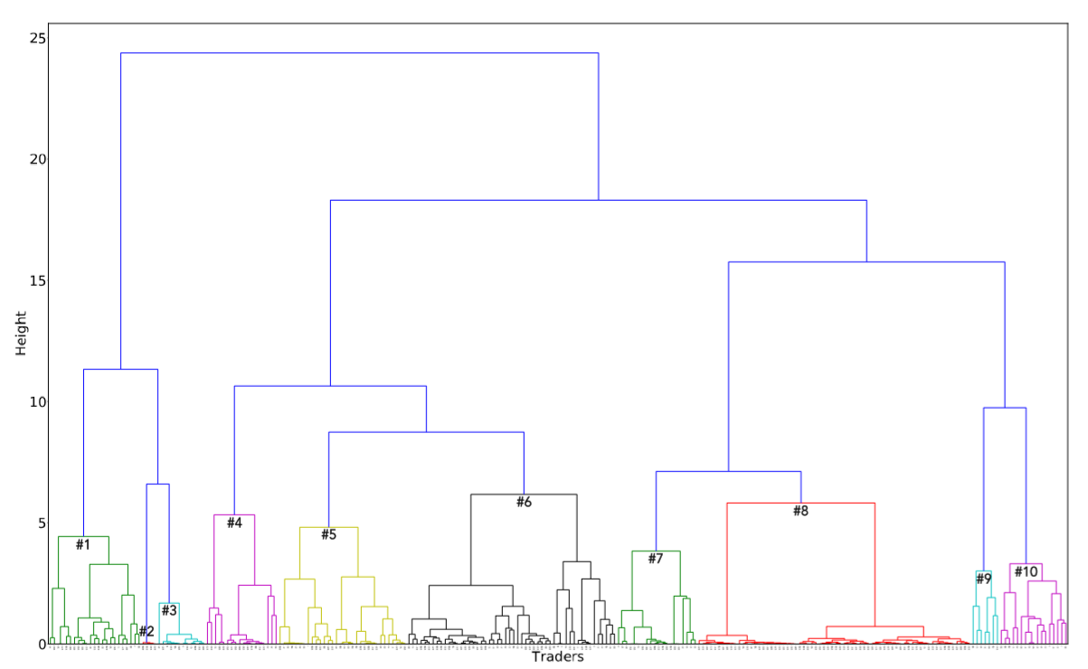
Figure 2 and Table 2 show our clustering results. Each color in Figure 2 indicates a corresponding cluster in Table 2. Among these clusters, we identified and selected one we assumed to be an HFT-MM cluster. Significant features in HFT-MM are a high cancel ratio and low inventory ratio. Clusters 5, 7, 8, 9, and 10 have high cancel ratios; clusters 3 and 9 have low inventory ratios. Thus, as an HFT-MM cluster, we selected cluster 9.
| #Cluster (Traders) | New orders | executed ratio | Canceled ratio | Trading tickers | VS usage | Market order ratio | Inventory ratio |
| 1 (23) | 3866.0435 | 0.5243 | 0.1247 | 8.9 | 1.48 | 0.0000 | 0.1364 |
| 2 (4) | 382847.0000 | 0.1971 | 0.0000 | 2614.3 | 1.00 | 0.0000 | 0.5966 |
| 3 (12) | 16488.0833 | 0.7675 | 0.2311 | 126.7 | 4.50 | 0.0000 | 0.0202 |
| 4 (18) | 847.3333 | 0.0748 | 0.6913 | 7.4 | 3.50 | 0.0207 | 0.8832 |
| 5 (32) | 67424.8750 | 0.1207 | 0.8347 | 787.2 | 7.16 | 0.0077 | 0.9294 |
| 6 (52) | 66695.8269 | 0.4376 | 0.4834 | 448.2 | 8.48 | 0.0423 | 0.9384 |
| 7 (20) | 26519.4250 | 0.0142 | 0.9820 | 57.2 | 4.05 | 0.0000 | 0.9438 |
| 8 (68) | 42106.8824 | 0.0218 | 0.9422 | 120.3 | 1.00 | 0.0000 | 1.0000 |
| 9 (7) | 96496.5714 | 0.0923 | 0.8489 | 21.7 | 10.00 | 0.0000 | 0.0502 |
| 10 (17) | 280585.0882 | 0.1387 | 0.8214 | 695.6 | 24.59 | 0.0003 | 0.1731 |
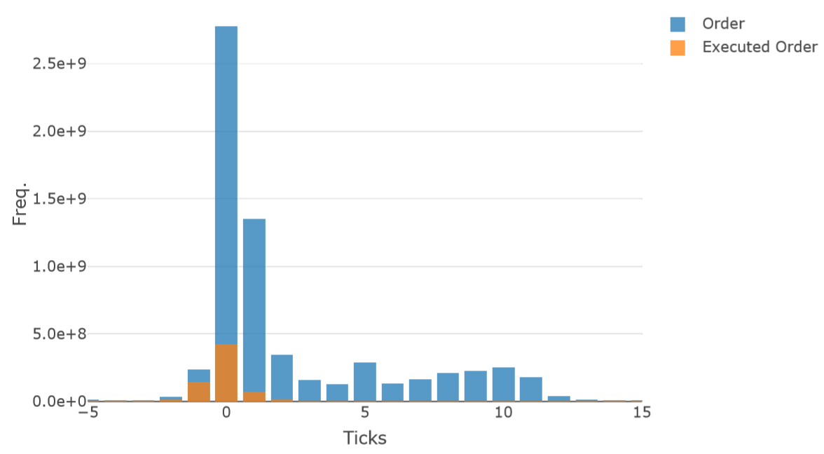
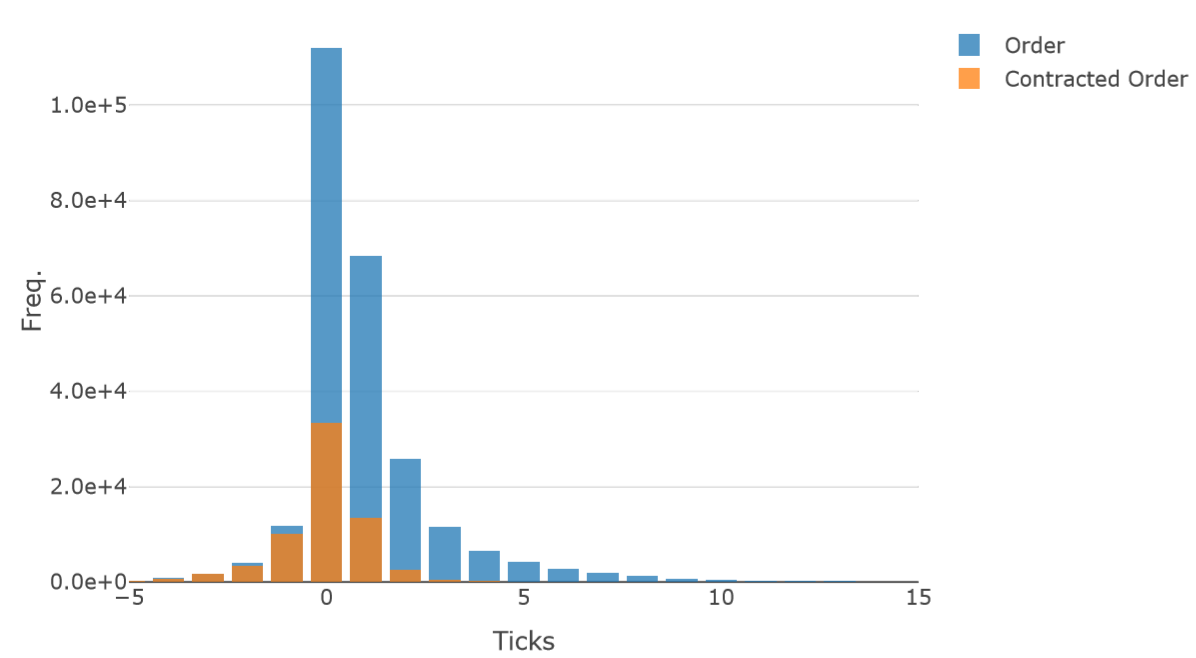
Next, we plotted the order placement distribution. Figure 3 shows our order price distribution analysis. This plot combines all the data from 21 business days and all the ticker data from traders in the HFT-MM cluster.
Brief discussion of clustering & order distribution analysis
The results here clearly show that many orders from HFT-MM traders (traders who were considered to be HFT- MM traders based on clustering) are placed near the market price. This allows for two conclusions. First, there are traders with HFT-MM features because the strategy of making several orders near the best or market price is typical of HFT-MM. Second, clustering analysis correctly selected HFT-MM traders. During clustering, we simply selected a cluster based on having checked only key indexes. However, the results indicate that the selected cluster was actually an HFT-MM cluster.
For a more accurate analysis, the analysis should be based not on ticks from the market price, but by ticks from the best price. However, the latter approach cannot be currently implemented owing to data characteristics and technical problems. That is, order-book reproduction data doesn’t have the information on the best prices, so we have to match them to the other order book databases. This process needs quite big computational resources.
Multi-Agent Simulation for HFT-MM Strategy in Artificial Market
In this section, we present our model for simulating artificial markets and its results. The importance of using numerical simulations, as mentioned in Section 1.1–1.5, is that we can conduct tests in a virtual market and engage in discussions that are not possible with traditional data analysis. In this paper, our main focus was to reveal the gap between real data and simulation analyses. Modeling HFT-MM in simulations is an essential task as the ratio of HFT in the financial market is showing a significant increase. Thus, in simulating an artificial market, we cannot ignore this type of HFT agent.
Model outline
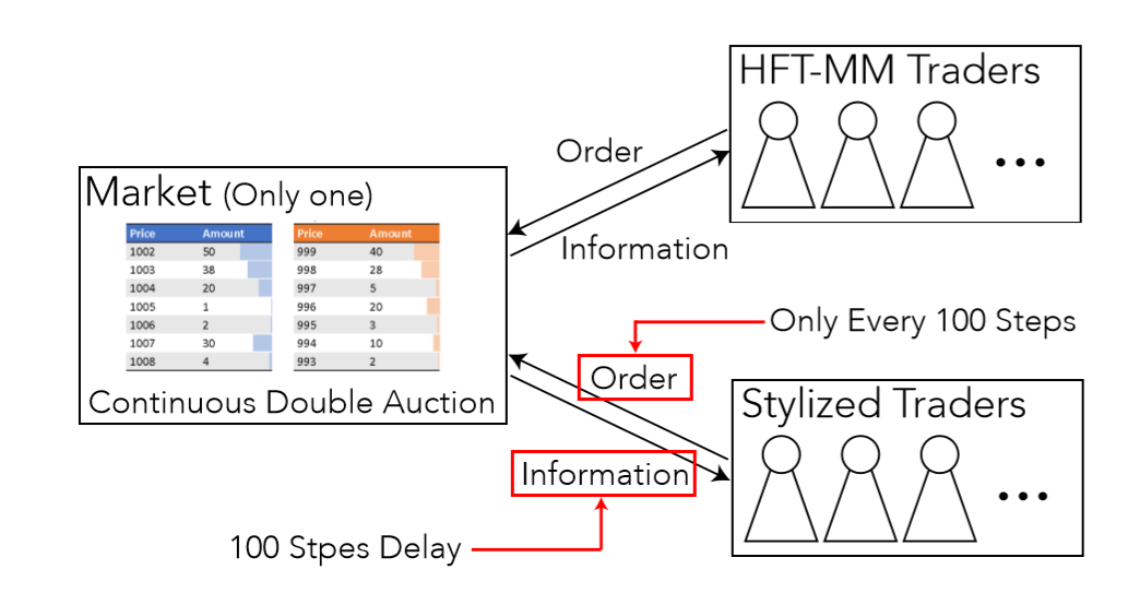
Figure 4 shows an outline of our simulation model. In our simulation, to simplify the model, we assumed there to be only one market with a continuous double auction system, as explained in Section 2.2 and Figure 1. We set the market start price to 400 and its fundamental price movement according to geometric Brownian motion with a standard deviation of 0.0001. We obtained this setting empirically by investigating real intra-day price changes, which are roughly about 1%, and considering the number of orders per step in simulations. There are two types of trader agents in our simulation model: HFT-MM and stylized. The most significant difference between HFT-MM and stylized traders is the access speed to markets, i.e., ordering speed and speed of accessing market information. In the real market, HFT-MM traders locate their Algo ordering servers on the place provided by stock exchange markets to reduce information and ordering latency. Thus, we built our model with latency and assumed that stylized trader agents have a 100-step information delay and can place their orders only every 100 steps. Other details regarding each agent type are provided in the following subsections.
Stylized trader agent model
For the stylized traders, we developed a trader model based on that reported in Torii et al. (2015). At time \(t\), stylized trader agent \(i\) decides its order price by the following equations, which consider fundamental, chartist, and noise factors.
First, we calculate the fundamental, chartist, and noise factors.
- Fundamental factor:
| $$F_t^i = \frac{1}{\tau^{*i}} \ln{\frac{p_{(t-100)}^*}{p_{(t-100)}}},$$ | (6) |
- Chartist factor:
| $$C_t^i = \frac{1}{\tau^i}\sum_{j=1}^{\tau^i} r_{(t-100-j)} = \frac{1}{\tau^i}\sum_{j=1}^{\tau^i}\ln{\frac{p_{(t-100-j)}}{p_{(t-100-j-1)}}},$$ | (7) |
- Noise factor:
| $$N_t^i \sim \mathcal{N} (0, \sigma),$$ | (8) |
Then, we calculate the weighted average of these three factors:
| $$\widehat{r_t^i} = \frac{1}{w_F^i + w_C^i + w_N^i} \left(w_F^i F_t^i + w_C^i C_t^i + w_N^i N_t^i\right),$$ | (9) |
In the next step, agent \(i\)'s expected price is calculated using the following equation:
| $$\widehat{p_t^i} = p_{(t-100)} \exp{\left(\widehat{r_t^i} \tau^i\right)}.$$ | (10) |
Then, using a fixed margin of \(k^i \in [0,1]\), the actual order prices are determined using the following rules:
- If \(\widehat{p_t^i} > p_t\), agent \(i\) places a buy order at the price
| $$\min{\left\{\widehat{p_t^i} (1-k^i), p_{t}^{\mathrm{buy}}\right\}}.$$ | (11) |
- If \(\widehat{p_t^i} < p_t\), agent \(i\) places a sell order at the price
| $$\max{\left\{\widehat{p_t^i} (1+k^i), p_{t}^{\mathrm{sell}}\right\}}.$$ | (12) |
Here, \(p_{t}^{\mathrm{buy}}\) is the best buy price, and \(p_{t}^{\mathrm{sell}}\) is the best sell price.
However, only using this routine based on that in Torii et al. (2015), stylized agents can make unlimited orders step by step. Thus, we implemented a simple cancel routine, whereby every 100 steps, when stylized traders can take action, stylized traders cancel all orders and make new orders according to the routine above.
The following are the parameters we employed for this type of trader: \(w_F^i \sim Ex(1.0), w_C^i \sim Ex(1.0), w_N^i \sim Ex(0.1), \sigma = 0.001, \tau^* \in [50,100], \tau \in [100,200]\). Other than weights, we mainly determined these parameters based on the work of Torii et al. (2015), and \(Ex(\lambda)\) indicates an exponential distribution with the expected value of \(\lambda\).
HFT-MM trader agent model
The HFT-MM trader agents in this study are based on Avellaneda & Stoikov (2008). Using a pricing calculation, we constructed the HFT-MM traders’ model.
First, we explain our calculation for pricing. At time t, agent i calculates the sell and buy prices by the following rules:
- Calculate agent i’s mid-price:
where \(\gamma^i\) is agent \(i\)'s risk hedge level, \(\widehat{\sigma^i}\) is agent \(i\)'s observed standard deviation in the last \(\tau^i\) steps, \(\tau^i\) is agent \(i\)'s time window size, as defined previously, \(T^i\) is the time until their strategy is optimized, and \(q_t^i\) is agent \(i\)'s inventory. \(T^i\) is the parameter in the optimization process for deriving this equation, which we set to \(1\).$$\widehat{p_{mid,t}^i} = p_t^* - \gamma^i \left(\widehat{\sigma^i}\right)^2T^iq_t^i,$$ (13) - Agent i’s price interval between sell and buy orders:
where \(k\) is a parameter for the order arrival time, which depends on \(Ex(k)\). In this simulation, we employed \(k=1.5\), which is the same as that used in Avellaneda & Stoikov (2008).$$\delta_t^i = \gamma^i \left(\widehat{\sigma^i}\right)^2T^i + \frac{2}{\gamma^i} \ln{\left(1+\frac{\gamma^i}{k}\right)},\label{eq:hft-delta}$$ (14) - Calculate agent i’s buy and sell price:
$$\widehat{p_t^\mathrm{buy}} = \widehat{p_{mid,t}^i} - \frac{\delta_t^i}{2},~~~ \widehat{p_t^\mathrm{sell}} = \widehat{p_{mid,t}^i} + \frac{\delta_t^i}{2}.$$ (15) - Then, agent i places a buy order at the following price:
where \(p_{t}^{\mathrm{buy}}\) is the best buy price, and agent \(i\) places a sell order at the following price:$$\min{\left\{\widehat{p_t^\mathrm{buy}}, p_t^\mathrm{buy}\right\}},$$ (16)
where \(p_{t}^{\mathrm{sell}}\) is the best sell price.$$\max{\left\{\widehat{p_t^\mathrm{sell}}, p_t^\mathrm{sell}\right\}},$$ (17)
In addition to price calculation, we implemented an order canceling routine. First, agents cancel orders whose orders to 10; if there are ten orders on the sell order book or ten orders on the buy order book, one order on the sell order book or buy order book is canceled. Moreover, all orders are subject to expiration. We set the expiration steps to be the same as the time window size of the agents. Thus, after this number of expiration steps has passed since the order was placed, the orders are automatically canceled.
Simulation Settings
In our simulation, there are 1,000 stylized trader agents and 10 HFT-MM trader agents. Each stylized trader agent has the opportunity to place orders every 100 steps. These opportunities do not arrive simultaneously, i.e., agent 1 has opportunities in the first step of every 100 steps, and agent 2 has opportunities in the second step of every 100 steps. This means, in every step, only 10 stylized traders and 10 HFT-MM traders are activated. The market mechanism is the continuous double auction system, as described in Section 2.2 and Figure 1. We implemented this mechanism in our simulation using the platform known as "PlhamJ" (Torii et al. 2019).
When the simulation starts, all stylized trader agents have 50 shares (at the beginning, $400 for each) and $30,000, and all HFT-MM trader agents have $50,000. At the beginning of the simulation, the share price is set to $400, so, 50 shares + $30, 000 = 50 x $400 + $30,000 = $50,000. These settings are not set empirically but set just for simulation working correctly because short selling is allowed. Moreover, these settings are the same as Torii et al. (2015).
In the simulation, there are 100 steps before the artificial market opening, 500 steps to market stabilization, and 10,000 steps in the test.
We ran the simulation 100 times. We also plotted the order placements.
Simulation results and brief discussion
Figure 5 shows the distribution of order price placements for the 100 simulations. This plot indicates how many ticks away from the best price the orders of the HFT-MM trader agents were. Many orders were placed near the best price because HFT-MM trader agents adopt strategies to do so. However, this distribution has a quite long tail. To identify the reason for the long tail, we performed another analysis.
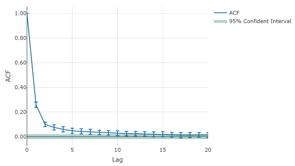
Figure 6 shows the autocorrelation function (ACF) for the absolute logarithm returns in one simulation run. This result indicates the presence of volatility clustering, which tend to have terms with high and low volatilities. Volatility clustering is listed as a stylized fact in Cont (2001) and Dacorogna et al. (2001).
Because of this volatility clustering, there is a highly volatile term for which increasing the σ value in Equation 14 causes HFT-MM traders to place orders far from the best prices.
Comparison of Data-based and Simulation Analyses
In Section 4.1–4.13, we showed the order placement plot of HFT-MM traders based on real financial market data. In Section 5.1–5.20, we introduced our simulation model and presented a plot of order placements by HFT-MM trader agents. In this section, we combine the results and compare them.
Order price distribution comparison
First, we generated a plot comparing the data mining and simulation results. To compare these plots, i.e., Figures 3 and 5, we normalized the order frequency by dividing by the maximum order frequency for each data type. The results show that these order frequencies were highest when the tick was 0, so we divided the order frequency by the frequency when the tick was 0 to obtain the relative frequency. Then, we generated the plot shown in Figure 7. Figure 7 shows a comparison of the relative order frequency of the actual data from the real financial market described in Section 4.1–4.13 and the simulation data described in Section 5.1–5.20. For the actual data from the real financial market, the horizontal axis is the number of ticks far from the market price. For the simulation data, however, the horizontal axis is the number of ticks away from the best price. This difference arises because we cannot obtain the best price from actual data owing to technical issues. Employing the market price in a simulation for this statistical analysis is inappropriate as the order book is thin and the spread is large because of the limited number of agents used. However, in the real financial market, HFT-MM trader agents tend to trade stocks that have high liquidity, so the market and best prices are not considerably different. Although we must address this problem, this difference is not significant.
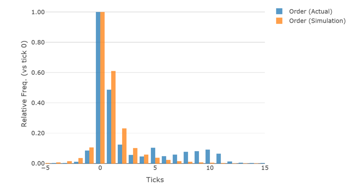
The plot in Figure 7 reveals that the order placement distribution by HFT-MM traders in the real market has significant tails on the right side. In the plot, when the number of ticks away is less than 4, the two plots are similar; however, when it is more than 5 ticks, the plots completely differ, and around 10 ticks away, the actual data have one local maximum. This phenomenon suggests that real HFT-MM traders combine the usual HFT- MM trade strategy in Avellaneda & Stoikov (2008) and another strategy in which orders are placed a little further from the best or market price. Before discussing this issue, we subjected these two distributions to statistical analysis.
Comparison by calculating entropy
To investigate the order distribution difference, we calculated the degree of entropy and performed t-tests.
First, we defined the order distribution range of the ticks. We set \(x\) as the number of ticks away from the market price (actual data) or the best price (simulation data). Then, we set the range to \(x \in [x_{\mathrm{min}}, x_{\mathrm{max}}]\).
Next, we calculated the ordering probabilities in the range:
| $$p_{x_{\mathrm{min}},x_{\mathrm{max}}}(x)=\frac{f(x)}{\sum_{i \in [x_{\mathrm{min}}, x_{\mathrm{max}}]}f(i)} ~~~ \left(x \in [x_{\mathrm{min}}, x_{\mathrm{max}}]\right),$$ | (18) |
Subsequently, we calculated the entropy.
| $$ E_{x_{\mathrm{min}},x_{\mathrm{max}}} = \sum_{x \in [x_{\mathrm{min}}, x_{\mathrm{max}}]}-p_{x_{\mathrm{min}},x_{\mathrm{max}}}(x)\log_2\left\{{p_{x_{\mathrm{min}},x_{\mathrm{max}}}(x)}\right\}.$$ | (19) |
Here, we used entropy as one index representing the ordering distribution. If the distribution is flat, i.e., the probability of each ordering action is almost the same, the entropy becomes high. On the other hand, if the distribution has a significant peak, the entropy becomes comparatively low. Actually, both actual and simulated ordering distribution has one significant peak. So, here, we can understand that the higher entropy means fat- tailed distribution. Moreover, the t-test between the entropy of actual and simulated ordering distribution can determine whether there is a significant difference between the two distributions.
Table 3 shows the results. Based on the t-test results, we found \(E_{-5,15}\) to show a significant difference, but \(E_{-2,5}\) did not. This reveals that the two ordering distributions for the actual and simulation data near the best or market price are not different, whereas the two ordering distributions over a wide range are significantly different. Specifically, the entropy of the actual data over a wide range was greater than that of the simulation data. This is consistent with the order placement plot from the actual data having a longer tail than that of the simulation data. Thus, in this section, the significant difference was verified statistically.
| Actual data | Simulation data | T-value | p | |
| \(E_{-5,15}\) | \(2.9289 ± 0.0207\) | \(2.3779 ± 0.0257\) | \(103.9132\) | \(4.2024\times 10^{-43}\) |
| \(E_{-2,5}\) | \(2.0874 ± 0.0186\) | \(2.0837 ± 0.0155\) | \(0.8209\) | \(0.4194\) |
Discussion and Conclusions
In our proposed method, we employed clustering and distribution analysis. Prior to clustering, we selected only high-frequency traders. Then, we performed a clustering analysis and selected one cluster, which we assumed to be HFT-MM traders based on some indexes. The results plotted in Figure Figure 3 clearly show an order frequency peak near the market price. It means that our clustering method worked correctly because this peak is assumed to be from the HFT-MM strategy. In addition, we carefully checked that this extraction of HFT-MM was correctly working to our purposes. As future work, in order to apply our method to other types of traders, we should improve the clustering method. There is a possibility that the same types of traders are placed in multiple clusters or that some HFT-MM traders are also placed in the other clusters we extracted. We should improve our clustering method by employing or integrating other methods, such as clustering or classification with a neural network or k-nearest.
Some considerations remain regarding our model and the results of our simulations. Our simulation is promising since it reproduced the order placement peak of the HFT-MM traders. Further, our simulation reproduced some stylized facts, such as volatility clustering. However, it must be said that achieving validity with this type of simulations is difficult. For instance, in our simulation, we employed only two types of trader agents. However, there are many trader types in real financial markets. Although we cannot create all agent types, we could consider employing additional types. If we added agent types, our model could approximate the real characteristics of markets in more detail. Moreover, this also could help improve the ordering action of other agents, so adding more realism to the mechanics of our simulated market.
Our comparison of the actual and simulation data yielded an interesting insight: Our simulation has high fidelity near the best price. However, far from the best price, there is a significant difference between actual data and our simulation. This difference may exist because real HFT-MM traders combine other strategies. The one possible strategy is placing and keeping orders away from the best price for faster extraction when the price changes dramatically according to time-priority rules. The financial market has a time-priority rule that means a fast order is executed faster under the same conditions. Thus, real HFT-MM agents are supposed to place some orders far from the best price. However, by simply modeling the artificial market without data, we may overlook these important factors. In fact, the previous work (Avellaneda & Stoikov 2008) overpassed this feature.
Therefore, in order to build a more dependable artificial market, it is essential to refer to real financial market data. Empirical data should be extensively used also when we do not merge the real data into simulation models. Conversely, if we build a model by focusing extensively on real data, the model could become overfitted with past data and result in irrelevant insights from the simulation.
To take advantage of the benefits of simulation, we should develop a technique that can merge simulation and real data. One possible solution is extracting principal components from real data and combining these with simulations. The current problem is that the model made by human model makers can overlook key features of markets by overimposing theories and biases. So, if models could be designed more technologically, these problems could be reduced. For instance, building a model by eploiting machine learning or deep learning on data could be an interesting option. In this respect, there are plenty of data in financial markets, such as tick data, that could be used to exploit the power of machine learning or deep learning to inform model building.
Moreover, we should try to focus also on other types of traders. This paper focused only on HFT-MM traders, whereas there are many types of traders and factors in the real financial market. The strategy of HFT-MM traders has been carefully modeled and is easily identified in real financial market data. However, dealing with traders or factors other than HFT-MM in the real financial market may prove more challenging.
In conclusion, in the next steps, we will try to build a method to implement real data to the simulation model without overfitting to the past record. Moreover, we will also extend and apply the method presented in this paper to the other type of traders.
Acknowledgements
We thank the Japan Exchange Group, Inc. for its provision of data. This research was supported by MEXT via Exploratory Challenges on Post-K computer (study on multilayered multiscale space-time simulations for social and economic phenomena).Notes
- This data is available for researchers under certain conditions.
References
AVELLANEDA, M. & Stoikov, S. (2008). High-frequency trading in a limit order book. Quantitative Finance, 8(3), 217–224. [doi:10.1080/14697680701381228]
BATTISTON, S., Farmer, J. D., Flache, A., Garlaschelli, D., Haldane, A. G., Heesterbeek, H., Hommes, C., Jaeger, C., May, R. & Scheuer, M. (2016). Complexity theory and financial regulation: Economic policy needs interdisciplinary network analysis and behavioral modeling. Science, 351(6275), 818–819. [doi:10.1126/science.aad0299]
BRAUN-MUNZINGER, K., Liu, Z. & Turrell, A. E. (2018). An agent-based model of corporate bond trading. Quantitative Finance, 18(4), 591–608. [doi:10.1080/14697688.2017.1380310]
CHIARELLA, C. & Iori, G. (2002). A simulation analysis of the microstructure of double auction markets. Quantitative Finance, 2(5), 346–353. [doi:10.1088/1469-7688/2/5/303]
CONT, R. (2001). Empirical properties of asset returns: Stylized facts and statistical issues. Quantitative Finance, 1(2), 223–236. [doi:10.1080/713665670]
EDMONDS, S. M. & Bruce (2005). Towards Good Social Science. Journal of Artificial Societies and Social Simulation, 8(4), 13: https://www.jasss.org/8/4/13.html.
FARMER, J. D. & Foley, D. (2009). The economy needs agent-based modelling. Nature, 460(7256), 685–686. [doi:10.1038/460685a]
GENÇAY, R., Dacorogna, M., Muller, U., Olsen, R. & Pictet, O. (2001). An Introduction to High-Frequency Finance. Academic Press. [doi:10.1016/b978-012279671-5.50004-6]
HIRANO, M., Izumi, K., Sakaji, H., Shimada, T. & Matsushima, H. (2018). Impact Assessments of the CAR Regulation using Artificial Markets. In Proceedings of International Workshop on Artificial Market 2018, (pp. 43–58).
HOCHREITER, S. & Schmidhuber, J. (1997). Long Short-Term Memory. Neural Computation, 9(8), 1735–1780. [doi:10.1162/neco.1997.9.8.1735]
HOSAKA, G. (2014). Analysis of high-frequency trading at Tokyo Stock Exchange. Securities Analysts Journal, 52(6), 73-82.
JAPAN Exchange Group (2017). Equities Trading Services | Japan Exchange Group: https://www.jpx.co.jp/english/systems/equities-trading/.
KRIZHEVSKY, A., Sutskever, I. & Hinton, G. (2012). Imagenet classification with deep convolutional neural networks. In Advances in neural information processing systems (pp. 1097-1105): http://papers.nips.cc/paper/4824-imagenet-classification-with-deep-convolutional-neural-networks.pdf . [doi:10.1145/3065386]
LUX, T. & Marchesi, M. (1999). Scaling and criticality in a stochastic multi-agent model of a financial market. Nature, 397(6719), 498–500. [doi:10.1038/17290]
MIYAZAKI, B., Izumi, K., Toriumi, F. & Takahashi, R. (2014). Change Detection of Orders in Stock Markets Using a Gaussian Mixture Model. Intelligent Systems in Accounting, Finance and Management, 21(3), 169–191. [doi:10.1002/isaf.1356]
MIZUTA, T. (2019). An agent-based model for designing a financial market that works well. Available at SSRN 3403461. URL http://arxiv.org/abs/1906.06000. [doi:10.2139/ssrn.3403461]
MIZUTA, T., Kosugi, S., Kusumoto, T., Matsumoto, W., Izumi, K., Yagi, I. & Yoshimura, S. (2016). Effects of Price Regulations and Dark Pools on Financial Market Stability: An Investigation by Multiagent Simulations. Intelligent Systems in Accounting, Finance and Management, 23(1-2), 97–120. [doi:10.1002/isaf.1374]
NAGUMO, S., Shimada, T., Yoshioka, N. & Ito, N. (2017). The effect of tick size on trading volume share in two competing stock markets. Journal of the Physical Society of Japan, 86(1), 014801. [doi:10.7566/jpsj.86.014801]
NANEX (2010). Nanex - Market Crop Circle of The Day: http://www.nanex.net/FlashCrash/CCircleDay.html.
NONAKA, Y., Onishi, M., Yamashita, T., Okada, T., Shimada, A. & Taniguchi, R. I. (2013). Walking velocity model for accurate and massive pedestrian simulator. IEEJ Transactions on Electronics, Information and Systems, 133(9). [doi:10.1541/ieejeiss.133.1779]
SAJJAD, M., Singh, K., Paik, E. & Ahn, C. W. (2016). A data-driven approach for agent-based modeling: Simulating the dynamics of family formation. Journal of Artificial Societies and Social Simulation, 19(1), 9: https://www.jasss.org/19/1/9.html. [doi:10.18564/jasss.2988]
TASHIRO, D. & Izumi, K. (2017). Estimating stock orders using deep learning and high frequency data [in Japanese]. In Proceedings of the 31nd Annual Conference of the Japanese Society for Artificial, (pp. 2D2–2).
TASHIRO, D., Matsushima, H., Izumi, K. & Sakaji, H. (2019). Encoding of High-frequency Order Information and Prediction of Short-term Stock Price by Deep Learning. Quantitative Finance, 19(9), 1499-1506. [doi:10.1080/14697688.2019.1622314]
TORII, T., Izumi, K., Kamada, T., Yonenoh, H., Fujishima, D., Matsuura, I., Hirano, M. & Takahashi, T. (2019). PlhamJ: https://github.com/plham/plhamJ.
TORII, T., Izumi, K. & Yamada, K. (2015). Shock transfer by arbitrage trading: analysis using multi-asset artificial market. Evolutionary and Institutional Economics Review, 12(2), 395–412. [doi:10.1007/s40844-015-0024-z]
TORII, T., Kamada, T., Izumi, K. & Yamada, K. (2017). Platform Design for Large-scale Artificial Market Simulation and Preliminary Evaluation on the K Computer. Artificial Life and Robotics, 22(3), 301–307. [doi:10.1007/s10015-017-0368-z]
UNO, J., Goshima, K. & Tobe, R. (2018). Cluster Analysis of Trading Behavior: An Attempt to Extract HFT [in Japanese]. In The 12th Annual Conference of Japanese Association of Behavioral Economics and Finance