RecovUS: An Agent-Based Model of Post-Disaster Household Recovery

Introduction

Population growth in hazard-prone areas together with the increase in severity of extreme events (Bergholt & Lujala 2012; Guha-Sapir, Hoyois, & Below 2016; Pravettoni 2009; Smith 2012) has raised the potential for disaster losses (Cutter et al. 2008; Schwartz 2006). Accordingly, a better understanding of the recovery process is necessary. Recovery process is a continuum of interdependent and mostly concurrent activities during pre-disaster preparedness and post-disaster short-term, intermediate, and long-term recovery. Among the components of this continuum, early-decided policies have a significant effect on the progress of recovery (FEMA 2011). In relation, analysis and modeling capabilities could help with capturing the dynamics of recovery and underpinning recovery plans.

Within a community recovery, housing restoration is of vital importance. Housing is a primary element of peoples’ lives, which influences their well-being by providing a safe and secure place and creating a positive sense of self-worth and empowerment (Bratt 2002). Furthermore, residential structures constitute the major share of building stock in the United States (Comerio 1998). In 2017, the number of U.S. houses was about 137 million units (USCB 2018), and their associated mortgage balance was reported at 9 trillion U.S. dollars in the second quarter of 2018 (FRBNY 2018). Additionally, the residential sector plays a significant role in shaping the built environment. Neighborhood characteristics such as availability of transportation systems, schools, employment opportunities, commercial establishments, recreational centers, etc. are influenced by households’ preferences and demands. These factors make housing a major sector of the U.S. financial and social infrastructure (Comerio 1998). Consequently, housing reestablishment influences overall recovery of a community through a ripple effect (Nejat & Damnjanovic 2012; Peacock, Dash, & Zhang 2007). Housing recovery is driven by many parameters and requires a collective endeavor to study. This makes it one of the most complex and least-studied topics in disaster recovery research (Drabek 2012; Ganapati & Ganapati 2008; Peacock, Dash, & Zhang 2007; Rubin 2009).

Recovery models aim to abstract and simulate the real world by including factors that affect the phenomenon of recovery. Miles & Chang (2006, Miles & Chang (2011), for example, applied stochastic simulation to simulate the recovery dynamics of households and businesses in the context of neighborhood and community conditions. Nejat & Damnjanovic (2012) developed an agent-based model using game theory to predict reconstruction decisions of households based on the status of their neighbors and future value of their own reconstruction (Nejat & Damnjanovic 2012). Miles (2017) developed a discrete event disaster recovery simulation framework (DESaster) that simulates owner, renter, and landlord households as the entities, recovery needs as the events, and human and financial resources as the resources. DESaster is capable of modeling households’ eligibility for financial assistance, sequential or parallel events, and stochasticity in the events’ durations (Miles 2017). Haer, Botzen & Aerts (2016) developed an agent-based model to examine the effectiveness of different flood risk communication strategies, as well as their circulation capabilities through social networks of households modeled as the agents. Filatova, Parker, & van der Veen (2011) used an agent-based model to research the effect of residents’ perceptions of flood risk on the value and development of coastal land in areas without flood-protection infrastructure. Magliocca et al. (2011) developed a coupled housing and land markets (CHALMS) agent-based model to simulate housing development in farmlands. The model includes three types of agents: housing consumer, farmer, and developer. Farmers decide whether to sell their lands by comparing the returns from farming to the expected price of their lands. The price of land is estimated based on the market supply-demand relationship. The housing density is decided by the developer based on the profitability of different housing types and consumers’ income, preferences for the house and lot size, and transportation costs (Magliocca et al. 2011). Magliocca & Walls (2018) adapted the CHALMS model to study land development in coastal areas. The model includes three types of agents: consumers, landowners, and developers. The model captures the interactions of agents to simulate market- and landscape-level outcomes and examine how the attractiveness of coastal amenities and the high risk of damage from storms collide to bring in the consumers’ buying decisions and their adaptive behaviors (Magliocca & Walls 2018). De Koning & Filatova (2020) developed an agent-based model to simulate relocation behavior of households residing in high-risk flood-prone areas. The model contains sellers and buyers as agents with heterogeneous risk perception and income whose interactions in the presence of repetitive floods produce the outmigration decisions (de Koning & Filatova 2020).

Households’ recovery decisions, however, are impacted by many parameters that their complete inclusion in a single model is infeasible. There are still gaps in the full understanding of post-disaster recovery and of how individual, communal, and organizational decisions interact to result in the overall recovery. Furthermore, integrating spatial aspects of recovery is an essential but under-researched concern. Therefore, the objective of the current research is to examine the impact of financial resources on homeowners’ recovery decisions and to capture the role of post-disaster functionality of infrastructure, the recovery of neighbors, and the functionality of community assets in the recovery of households with heterogeneous preferences. For this purpose, RecovUS, an agent-based model of recovery, was developed. Mitigation/recovery decision-makers can utilize RecovUS to prioritize and underpin recovery policies based on distinct household characteristics to ensure an enhanced community recovery program as proactive and data-informed recovery plans can majorly impact the overall recovery of a community (Hirayama 2000; Ingram et al. 2006).

This study focuses on owner-occupied single-family detached homes. The rationale behind this selection was the prevalence of this type of housing in the United States’ residential sector. Moreover, other housing types have different and more complicated recovery behaviors, stemming from their sophisticated ownership patterns, which require a different research methodology (Zhang & Peacock 2009). This study directly involves insurance companies and public agencies providing housing financial assistance and indirectly engages the latter via restoration of infrastructure and community assets. Additionally, the model includes spatial aspects of recovery by capturing the effect of recovery of neighbors and neighborhood community assets on households’ recovery decisions. Although this scope is not a representation of the total residential sector, it addresses a major share. Additionally, it provides a framework to examine emergent recovery behaviors in the presence of recovery drivers and uncertainties.

In the following sections, the related literature is outlined first. Then, the methodology of the research is presented, and the process of collection and generation of data is described. Next, the model outcomes are presented and discussed. Finally, the research limitations and contributions are summarized and future lines of study are proposed.

Literature Review

Drivers of recovery

The parameters that affect housing recovery can be classified into three general categories concerning their relationship with households, including internal, interactive, and external drivers (Moradi et al. 2020a). Internal drivers are the factors directly related to households, such as household attributes and level of damage caused by a disaster. Different socioeconomic conditions differentiate the resilience of households (Burton 2015; Moradi, Vasandani, & Nejat 2019) and contribute to the emergence of dissimilar patterns of recovery. Economic status, for example, affects households’ post-disaster recovery. Individuals with greater financial power may apply disaster mitigation more often and consequently be less impacted (Hunter 2005), while lower incomes are more likely to experience a slower recovery (Peacock, Van Zandt, Zhang, & Highfield 2014). Level of educational attainment has also been reported to positively influence restoration (Burton 2015). Further, racial disparity was found as the major cause of the lengthy process of recovery after Hurricane Andrew (Zhang & Peacock 2009) and Hurricane Katrina (Bullard & Wright 2009). Age (Henderson, Roberto, & Kamo 2010; Sanders, Bowie, & Bowie 2004), gender (Nejat, Binder, Greer, & Jamali 2018), marital status (Nejat & Ghosh 2016), and household size (Nejat et al. 2020; Sadri et al. 2018) are other attributes that can affect recovery. Another important driver is the damage severity. The effect of the damage can last for several years after a disaster (Hamideh, Peacock, & Zandt 2018; Peacock et al. 2014). A higher relocation ratio has been reported for more-impacted residents (Mayer et al. 2020; McNeil, Mininger, Greer, & Trainor 2015; Myers, Slack, & Singelmann 2008). Additionally, among households who stay, restoration could take longer for those whose properties have sustained more damage (Sadri et al. 2018).

Interactive drivers are developed through the interaction of individuals with their community. Social capital, place attachment, and recovery of neighbors are among these drivers. Several studies have demonstrated the role of social capital in post-disaster recovery (Aldrich 2011; Burton 2015; Sadri et al. 2018), as it facilitates the achievement of common goals through mutual communications (Jamali & Nejat 2016) and provides informal resources for recovery (Airriess et al. 2008; Aldrich 2010). Place attachment also affects households’ recovery decisions. Residents are connected to their place of living via the resources as well as the sense of identity offered by the neighborhood (Jamali & Nejat 2016). Sense of place has been reported as a key player in decisions of households against relocation (Binder, Baker, & Barile 2015; McNeil et al. 2015). Additionally, households’ recovery decisions are influenced by their neighbors. Recovery of neighbors relays a positive message on restoration of the neighborhood and encourages other residents to repair/reconstruct (Nejat & Damnjanovic 2012; Rust & Killinger 2006).

External drivers are provided by different public, private, and non-profit organizations. Examples include financial resources and restoration of infrastructure and community assets. Financial aids provided through insurance policies, disaster loans, and public funds enhance the progress of restoration (Nejat & Ghosh 2016). Distribution of these resources affects the pattern of recovery such that regions with less assistance may experience a higher rate of relocation (Kamel & Loukaitou-Sideris 2004). Further, infrastructure and community assets, such as transportation systems, commercial features, schools, and healthcare facilities, provide services vital to the residents and which address their regular and recovery-specific needs (Aghababaei et al. 2020; Comerio 2014; Ronan & Johnston 2005; Xiao et al. 2018). Additionally, post-disaster functionality of infrastructure and community assets influences households’ perception of their neighborhood reestablishment and can impact their decisions in favor of or against repair/reconstruction (Dehghani & Shafieezadeh 2019; Moradi 2020b; Nazarnia, Sarmasti, & Wills 2020).

Perceived neighborhood

People differ in how they delineate their neighborhood even though they may live in geographic proximity (Coulton et al. 2001). Consequently, features they expect from their neighborhood, as well as its boundaries, may be dissimilar (Nejat 2018; Nejat, Moradi, & Ghosh 2019). Recognizing these preferences and integrating them into the modeling can provide a more realistic picture of the residents’ needs and priorities (Moradi et al. 2019). Various factors affect the perception of a neighborhood, such as residents’ sociodemographic attributes, neighborhood characteristics, and physical elements. Individuals with a longer duration of residence and higher income, education, and engagement in neighborhood activities may perceive a larger neighborhood (Coulton, Jennings, & Chan 2013). Racial similarities can also cause adjacent areas to be included in or excluded from an individual’s perceived neighborhood (Campbell et al. 2009; Krysan 2002). Further, residents may perceive a smaller neighborhood in high-density and mixed-used areas (Coulton et al. 2013) and a smaller neighborhood in suburban regions (Haney & Knowles 1978). Physical elements such as streets, parks, and rivers can also affect perceived neighborhood boundaries (Campbell et al. 2009).

Nejat et al. (2019) developed an index, Anchors of Social Network Awareness index (ASNA-i), to classify households based on the perception of their neighborhood. The index considers three classes of households: index 1, or infrastructure-aware class, is characterized by its preference for transportation and geographical features; index 2, or social-networks-aware class, opts for friends and families and neighborhoods; and index 3, or community-assets-aware class, prefers community assets and public services and safety. The classification is estimated by a latent class regression model that uses the logarithm of the population density of a county of residence, household income, and householder educational attainment and race as covariates (Nejat et al. 2019). Perceived neighborhood areas and their relationships with ASNA indexes have also been investigated by Nejat (2018) and Moradi et al. (2020).

Research Methodology

RecovUS was developed at the household level to simulate post-disaster recovery decisions of households residing in their own single-family houses. Each household is represented in the model by an agent located on the polygon centroid of its home. A household agent possesses particular attributes, including characteristics of the householder (e.g., income and ASNA index) as well as information on the house in which it resides (e.g., pre- and post-disaster value and square footage). Based on its specific characteristics, each agent senses the environment and/or other agents, evaluates the conditions, and decides for its recovery. Recovery choices are repair/reconstruction of the damaged house, waiting without repair/reconstruction, or selling the house (and relocating).

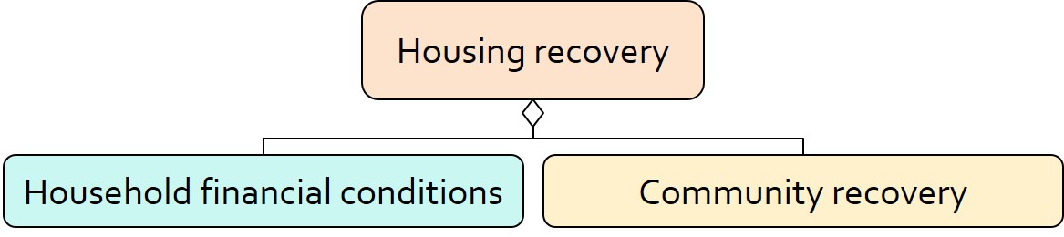
RecovUS is founded on the assumption that housing recovery is a function of households’ financial conditions and community recovery. It assumes that a household would meet the prerequisites of repair/reconstruction if 1) it has enough financial resources, and 2) its community has recovered adequately (Figure 1).

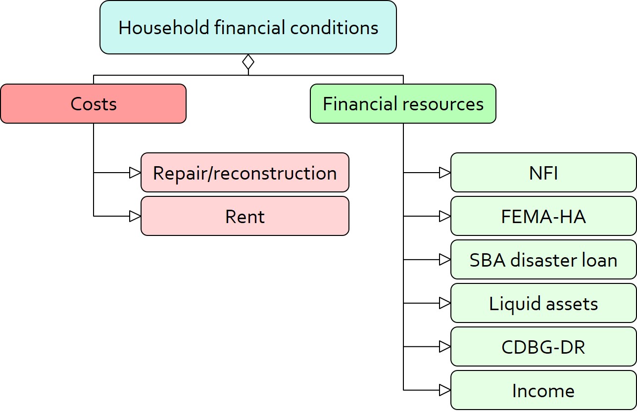
A household’s financial conditions are evaluated by two categories of variables: costs and resources (Figure 2). Costs include repair or reconstruction costs and rent of another property when the primary house is uninhabitable. Resources comprise the money required to cover the costs of repair/reconstruction and to pay the rent (if necessary). The repair/reconstruction resources include settlement from the National Flood Insurance (NFI), Housing Assistance provided by the Federal Emergency Management Agency (FEMA-HA), disaster loan offered by the Small Business Administration (SBA loan), a share of household liquid assets, and Community Development Block Grant Disaster Recovery (CDBG-DR) fund provided by the Department of Housing and Urban Development (HUD). Furthermore, household income determines the amount of rent the inhabitants can afford.

Community conditions are assessed for each household based on the restoration of specific anchors (Figure 3). ASNA indexes (Nejat et al. 2019) are estimated to identify the category of anchors important to the recovery decision of each household. Accordingly, households are indexed into three classes for each of which recovery of infrastructure, neighbors, or community assets matters most. Furthermore, among similar anchors, those anchors are important to a household that are located in its perceived neighborhood area (Moradi et al. 2020; Nejat 2018).

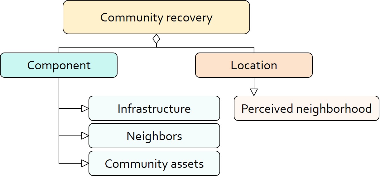
Figure 4 shows the steps of evaluating the recovery criteria and predicting the households’ decisions. In each time step, the program implements the following procedure:

1. The algorithm starts with reimbursing financial aid to the eligible households that have been damaged by the disaster. These aids include NFI settlements, FEMA-HA, SBA loans, a share of liquid assets that households spend on recovery, and CDBG-DR assistance. The resources are reimbursed in sequence in order not to duplicate each other.
2. Next, the model compares each households’ available financial resources to the damage cost. If the financial criterion is not satisfied (i.e., the available financial resources are not enough to cover the repair/reconstruction costs), the program evaluates the habitability of the house. If it is habitable, the household is expected to wait with a probability of r₁ %, but it also has the alternative of selling the property with a probability of (100-r₁)%. If the house is uninhabitable, two additional conditions are evaluated. If the household can afford to pay for the rent of another property and a vacant rental unit is also available, the options would be waiting or selling (like the previous case), but if either is not met, the only option would be selling the house.
3. If the financial criterion is satisfied, the community criterion is evaluated. Based on the ASNA index of a household, restoration of infrastructure, neighbors, or community assets is compared to its desirable threshold (adq_infr, adq_nbr, and adq_cas, respectively). If the perceived community has adequately recovered, the household is expected to decide in favor of repair/reconstruction with a probability of r₂%, though it would also have the alternative of selling with a probability of (100-r₂)%. However, if community recovery is inadequate, the model proceeds like the situation in which financial resources were not enough (no. 2 above). In other words, habitability, rent affordability, and vacancy are checked, and the household decides to wait or sell the house.
4. If a house is sold, the buyer would decide to repair/reconstruct the house with a probability of r₀%, or wait (or sell again) with a probability of (100-r₀)%.

The thresholds r₀, r₁, r₂, adq_infr, adq_nbr, and adq_cas are model parameters and their values are determined by calibration. The model algorithm is discussed in detail in (Appendix, using the Overview, Design concepts, and Details (ODD) protocol (Grimm et al. 2006; Grimm et al. 2020).

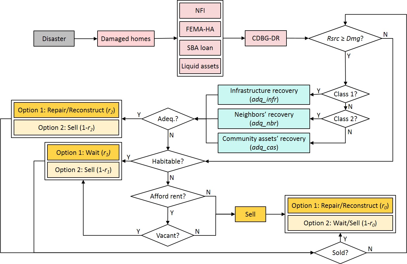
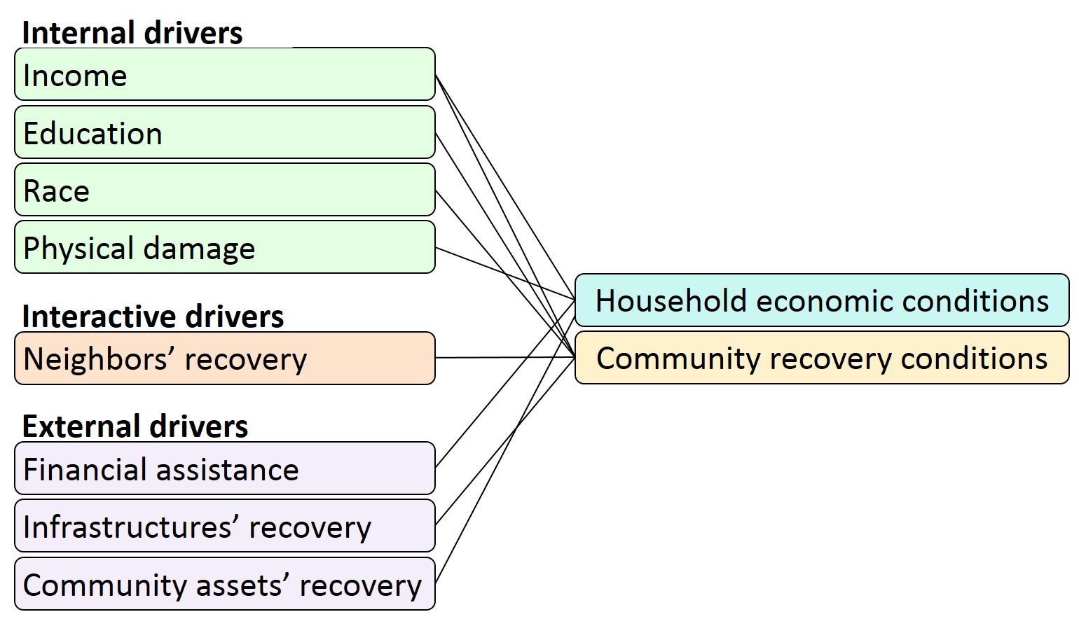
Figure 5 illustrates the linkage of drivers of recovery to the model. Internal drivers relate to both financial and community conditions. Education level, race, and income connect to community conditions by identifying the anchor-based index of a household and its perceived neighborhood area. Physical damage is tied with financial conditions due to its association with repair/reconstruction costs. Also, the level of damage determines whether a home is habitable or the household needs to rent another residence. Furthermore, household income is related to financial conditions by estimating the amount of resources available for repair/reconstruction and the ability to pay for rent. Interactive drivers are coupled with community conditions through the influence of neighbors’ recovery on recovery decisions of the index-2 households. Finally, external drivers relate to both financial and community conditions. The linkage to the former is via the provision of housing financial assistance, and to the latter through the effect of recovery of infrastructure and community assets on recovery decisions of index-1 and index-3 households.

Data

Recovery of Staten Island, New York after Hurricane Sandy was selected as the case study to provide the input data. Sandy was a hurricane/post-tropical cyclone that hit the eastern coast of the United States on October 29, 2012. It was one of the largest Atlantic tropical storms that extended into a territory with a diameter of 1,000 miles and affected 24 States. The highest storm surge was recorded nine feet along the shoreline in Manhattan and Staten Island. Sandy resulted in at least 147 deaths, caused loss of power in 8.5 million houses and $65 billion in damage, and damaged or destroyed 650,000 houses and hundreds of thousands of businesses (GAO 2015; HRD 2019; NOAA & NWS 2013).

The input data for the model is classified into two general categories of non-disaster-related and disaster-related data. The non-disaster-related data includes information that does not change based on a specific disaster, such as household income, educational attainment, race, and housing characteristics. The disaster-related data, on the other hand, includes information that differs based on the hypothesized disaster case, such as damage to houses, housing financial assistance, and damage and restoration of infrastructure and community assets. The input data consists of:

1. Housing attributes, including Staten Island single-family detached homes, their spatial location, level of damage caused by Hurricane Sandy, and restoration status after two years.
2. Household attributes, including household income and ASNA index.
3. Financial resources, including distribution of NFI, FEMA-HA, SBA loan, CDBG-DR, and liquid assets.
4. Households’ financial ability to pay rent.
5. Damage to infrastructure and community assets and their restoration progress.

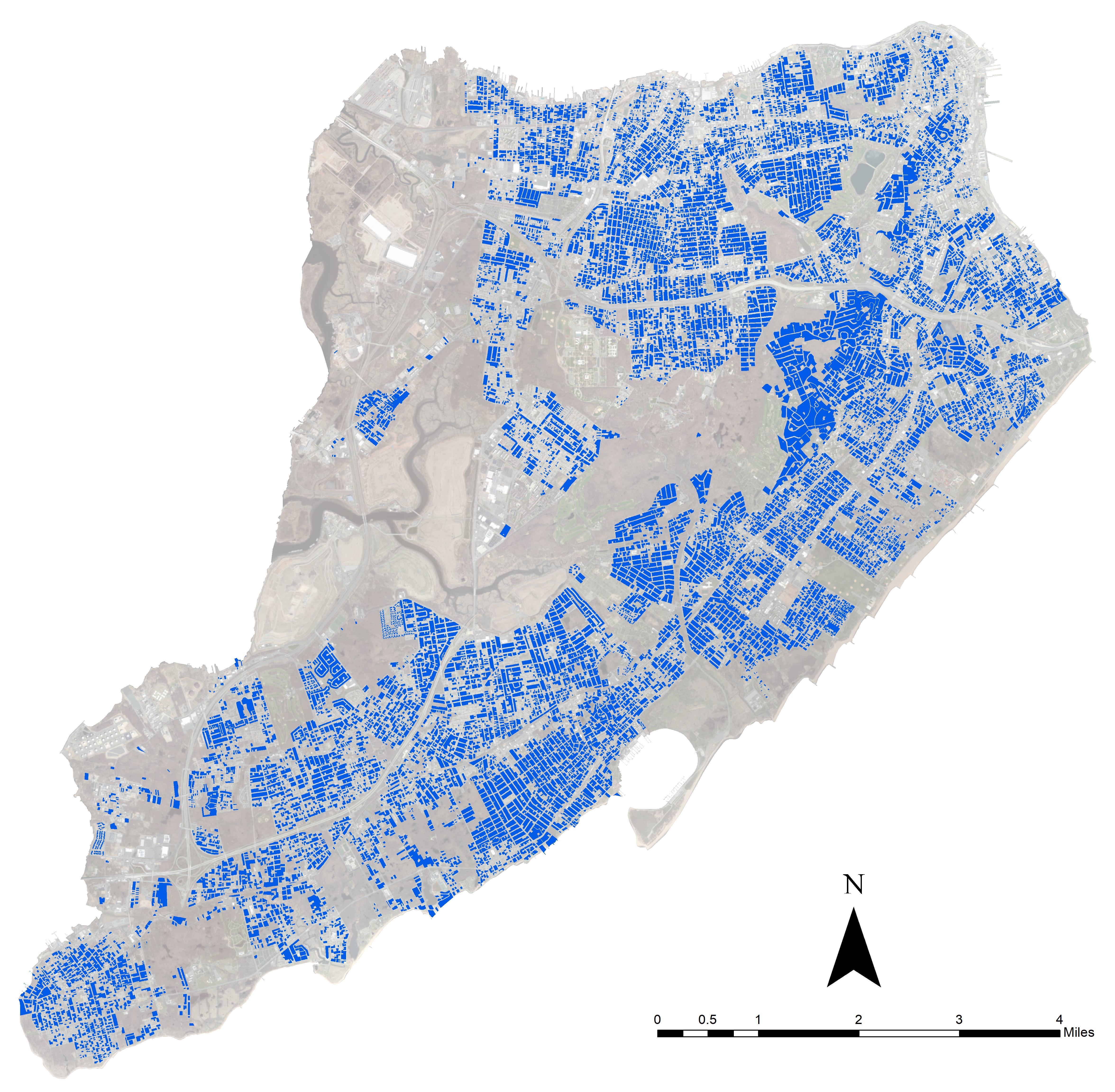
While this section provides a brief description of the data, a more detailed explanation is provided in Appendix (section Input data). The first category of data is housing attributes. This information was extracted from the New York City tax assessment data (NYC 2019a). Cleaning the data to include only single-family detached homes of Staten Island resulted in 74,604 houses. Improvement market values for each house in each year was calculated by subtracting the land market value from the total market value. The improvement value estimates the worth of additions to the land, mainly due to the structure. The improvement values were discounted back to a common time (August 2011) using monthly Consumer Price Indexes (CPIs) for housing in New York, Newark, and Jersey City (BLS 2019) to have the same basis for comparison. The discounted improvement market (DIMP) values were used to estimate the damage to the properties. If the DIMP value of a house showed a decrease in the first post-Sandy year compared to the pre-Sandy year, the house was assumed damaged and the amount of damage was estimated as the difference between the pre- and post-sandy DIMP values. Additionally, once the DIMP value in the subsequent years reached or exceeded the pre-Sandy DIMP value, the house was assumed to have been completely restored to its pre-disaster condition. The data were joined to the shapefile of the lots’ polygons (NYC 2019b) using ArcGIS Desktop 10.3.1 (ESRI 2015) to provide the input file for RecovUS (Figure 6). More information is presented in the Appendix (section Input data: Housing attributes).

Household income and the householder ASNA index are of the other inputs. Household income is applied to estimate households’ liquid assets and renting power and to control the eligibility criteria to receive financial assistance. Additionally, household income together with the population density of county of residence, householder educational attainment, and householder race is used to estimate ASNA indexes based on the latent class regression model proposed by Nejat et al. (2019), the details of which are provided in the Appendix. While population density is simply calculated, data on the other three covariates are not generally available at the household level. In the current research, this data was synthetically generated by Iterative Proportional Fitting (IPF) of the 2013 census data on household income, educational attainment, and race (USCB 2013a, 2013b, (2013c), as explained in the Appendix. To reduce RecovUS runtime, ASNA indexes were estimated in advance from the covariates and were joined with the household income to the lots’ shapefile using ArcGIS. Please see the Appendix (section Input data: Household attributes) for more explanation.

Another category of input is the data on financial resources including NFI, FEMA-HA, SBA loan, CDBG-DR, and liquid assets. The National Flood Insurance Program (NFIP) paid 32,360 losses (totaling $8.80 billion) in the 16 states impacted by Hurricane Sandy (III 2019a, 2019b). In the absence of higher-resolution data, 80% of the houses located within areas at high risk of flooding (FEMA 2019a; Shawnee County 2019) were assumed to be reimbursed by the NFIP. Additionally, zip-code level data on reimbursement of FEMA-HA and SBA loan were obtained from FEMA (2019b) and SBA (2014), respectively. Additionally, zip-code-level data on the distribution of CDBG-DR funds to single-family houses was obtained from NYC (2019c). Furthermore, the 2013 census data on households’ wealth (USCB 2014) was used to estimate households’ net worth based on their income. Households were assumed to consider a share of their net worth (1-20%) as the liquid assets assigned for repair/reconstruction costs. Please see the Appendix (section Input data: Financial resources) for more detail. The financial ability of households to pay rent is another input data. Household financial power regarding rent was assumed to be a fraction of the household income (up to 40%). Additionally, the amount of rent was estimated using the HUD’s Fair Market Rent (FMR) for Staten Island (HUD 2019). Comparison of a household financial power to the amount of rent determined whether a household could afford to pay the rent. More explanation is provided in the Appendix (section Input data: Rent).

The last group of input is the data on damage and restoration of infrastructure and community assets. This data was estimated from qualitative reports. A report published by the City of New York (NYC 2013) describes the important transportation infrastructure and community assets. For example, it mentions that a “transportation asset on the East and South Shores is the SIR, a 14-mile commuter rail line operated by the Metropolitan Transportation Authority (MTA)…”. The report then explains what happened in Sandy: “Major damage also occurred at the SIR’s operations and maintenance facilities, limiting service in the days after the storm (ultimately, full service was only restored in mid-December)” (NYC 2013). The authors used these descriptions to subjectively estimate the infrastructure damage every three months after the disaster. For example, it was assumed that the SIR was 80% unfunctional immediately after the hurricane (“Major damage”) and was completely restored within the first three months (“full service … in mid-December”). The estimated damage was also checked for consistency with other reports (Kaufman & Shaby 2013), where possible. Since the items in the report were major infrastructures that affected most residents, the average damage to the infrastructure system (rather than individual infrastructures) was calculated and fed into the model. Damage to the community assets was estimated for 135 community assets using a similar approach and joined to their shapefile (NYC 2019b). RecovUS evaluates recovery of community assets based on the geographic location of the assets since they were assumed to mostly serve the local residents. More information is provided in the Appendix (section Input data: Infrastructure and community assets).

Results and Discussion

Model calibration

Six thresholds in the model affect households’ decisions: adq_infr, adq_nbr, adq_cas, r₀, r₁, and r₂. The values of these variables are obtained by calibrating the model. The objective of calibration (also called training in the field of machine learning) is to optimize the parameters such that the model would have the least (training) error value (i.e., the overall model predictions would have the least difference with empirical data). Herein, the model predictions are recovery decisions of households (repair/reconstruct or not) at the end of the 24^th month and the empirical data include the recovery status of houses estimated from tax assessment data as described previously. The model was run using the systems of Texas Tech High-Performance Computing Center (HPCC 2019). Calibration started on a broader range of values for the parameters and a smaller number of repetitions and continued with narrowing the range of values and increasing the number of repetitions (Table 1). The reason for this configuration was to evaluate the predictions of the model on a wide range of values and accommodate the HPCC runtime limitations. The predictions from each set of values were averaged on the number of repetitions to obtain the average number of repairs/reconstructions. Then, the prediction error, called the training error, was calculated by comparing the average number of repairs/reconstructions predicted by the model with the number of repairs/reconstructions from the empirical data. Table 2 presents the set of values that yielded the minimum average training error (averaged over 1,000 repetitions). The small error of -0.21% indicates a good fit to the data.

Table 1: Settings of the model parameters for calibration

Setting	adq_infr	adq_nbr	adq_cas	r0	r1	r2	Repetitions
1	55:5:100	55:5:100	55:5:100	55:5:95	55:5:95	55:5:95	1
2	0:5:100	0:5:100	0:5:100	30:5:70	95	95	10
3	0:10:100	0:10:100	0:10:100	35	95	95	10
4	50	30:5:100	50	35	95	95	100
5	50	40	50	35	95	95	1000

Table 2: Selected values for the model parameters.

Dataset	adq_infr	adq_nbr	adq_cas	r0	r1	r2	Training error (%)
All	50	40	50	35	95	95	-0.213

The value of 95% obtained for r₁ through calibration implies the probability of waiting (against selling) for a household whose recovery criteria have not been met yet is 95%. Similarly, the value of 95% for r₂ means the probability of repair/reconstruction for a household with satisfied recovery criteria is 95%. The calibrated values indicate that the behavior predicted by the model corresponds to its fundamental hypotheses, meaning that once both criteria are met, households mostly decide to repair/reconstruct (r₂ = 95%). Conversely, when either criterion is not satisfied, repair/reconstruction does not progress much (r₁ = 95%). These results are also consistent with the pattern reported in the literature. According to Peacock et al. (2014), for instance, higher incomes among households impacted by Hurricane Andrew in Miami-Dade repaired/reconstructed more quickly. Kamel & Loukaitou-Sideris (2004) studied the recovery of Los Angeles following the Northridge earthquake and reported a lower recovery in neighborhoods underfunded by federal assistance programs. Similarly, Nejat & Ghosh (2016) suggested that availability of financial resources affected decisions of Staten Island residents, who had been impacted by Hurricane Sandy, in favor of repair/reconstruction. Additionally, recovery of neighbors, infrastructure, and community assets has been reported to positively influence housing reconstruction (Burton 2015; Comerio 2014; Rust & Killinger 2006).

The value of 35% for r₀ entails that the probability of buyer repair/reconstruction is about half the probability of waiting. The empirical data also supported this value. The tax assessment data (NYC 2019a) includes the names of properties’ owners in each fiscal year. The analysis of the data revealed that about 67% of the damaged properties whose owners had changed after Sandy (sold the property) had not yet recovered until the second year (equivalent to r₀ = 33.12%). A similar ratio has also been reported for the recovery of auctioned houses in Long Island (Polsky 2020).

Furthermore, the analysis showed low sensitivity of the model to changes in adq_infr and adq_cas. The reason for the former is the rapid recovery of infrastructure within the first few months. Thus, no matter what value was selected for adq_infr, the criterion of community recovery for index-1 households was satisfied in the initial time steps. Additionally, since index-3 households constitute a small share of the population (about 4%), change in the value of adq_cas does not significantly affect the overall output. Finally, the optimized value for adq_nbr implies that at least 40% of neighbors should restore in order to satisfy the community criterion for index-2 households.

Validation

The small training error obtained for RecovUS (-0.21%) means the model is not underfitting the data, i.e., using the input dataset together with the values obtained for the parameters from calibration would lead to a prediction that adequately represents the pattern observed in the empirical data (Goodfellow, Bengio, & Courville 2016). However, measuring the performance of a model against the same dataset used for calibration may result in an optimistic conclusion. The more meaningful approach is to validate the model, i.e. examine generalization performance of the model over previously unobserved datasets to assure it would not overfit the data (Theodoridis 2015). A small gap between training error and test error would satisfy this purpose (Goodfellow et al. 2016). This study applied the k-fold cross-validation method, which is a common technique for estimating a model’s test error. The idea is to randomly divide the dataset into k subsamples with roughly equal sizes, form a training set by deleting one group, and assign the deleted group to the test set. The model is calibrated over a training set and is used over the corresponding test set to obtain the prediction error, also known as the test error. The test errors are finally averaged on the number of sets (k) to yield an average estimation of the generalization error (Theodoridis 2015; Twomey & Smith 1997; Wold 1978).

The dataset was divided into four subsamples constituting the four training and test sets (Table 3 and Figure 7). Count and Ratio in Table 3 represent the number and percentage of damaged houses in each dataset, respectively. Since RecovUS captures the spatial aspect of recovery by evaluating the recovery of neighbors and community assets, subsamples are four geographic regions of the dataset (zip codes) with almost the same number of damaged houses rather than sparse samples. As depicted in Table 3, each test set consists of about one-fourth (since k = 4) of the total number of damaged houses.

Table 3: Training and test sets for k-fold cross-validation

Dataset	Train			Test COLON 2
		Count	Ratio (%)		Count	Ratio (%)
All	42645	100.00		-	-
Set 1	30771	72.16		11874	27.84
Set 2	32617	76.48		10028	23.52
Set 3	31430	73.70		11215	26.30
Set 4	33117	77.66		9528	22.34

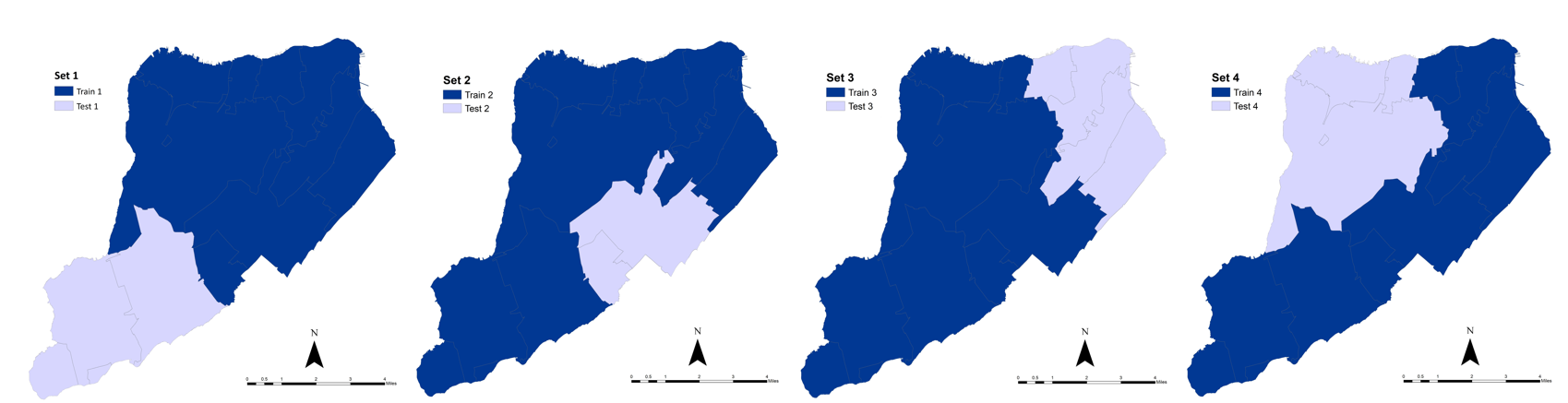
Using the k-fold cross-validation method, the model was first calibrated using one training set at a time to obtain the optimized values for the parameters. Calibration was performed using a similar procedure as explained before. Table 4 summarizes the results. The model was run over one of the training datasets and a range of values for the model parameters (100 repetitions on each set of values). The average error, called training error, was then calculated by comparing the average number of repairs/reconstructions predicted by the model (averaged on 100 repetitions) with the number of repairs/reconstructions from the empirical data. The set of values associated with the minimum training error was selected as the calibrated values. The calibrated values were again used over the same training dataset, but the model was run 1,000 times to calculate and report a more accurate training error (Table 4). Then, the calibrated model was run 1,000 times over the corresponding test dataset, and the average error, called the test error, was calculated by comparing the number of repairs/reconstructions predicted by the model with the number of repairs/reconstructions from the empirical data. This procedure was repeated over the four folds of the data and the associated errors were calculated. Finally, the model's test error, calculated by averaging the four test errors weighted by the number of samples, was obtained to be equal to 0.44% (Table 4). The small difference between training and test errors (0.66%) assures that the model generalizes well on unobserved data.

Table 4: Model parameters

Dataset	adq_infr	adq_nbr	adq_cas	r0	r1	r2	Training error (%)	Test error (%)
Set 1	50	90	50	35	95	95	0.358	-17.199
Set 2	50	85	50	30	90	90	0.123	-0.201
Set 3	50	85	50	35	90	85	0.017	14.393
Set 4	50	40	50	40	95	95	0.138	6.687
Average test error (%)								0.443

Computational experimentation

Two series of sensitivity analyses were performed to evaluate the relative importance of model variables and assumptions. Herein, relative importance means the amount of which a variable or assumption affects the model output in terms of damaged houses repaired/reconstructed. In the first series of analysis, the six thresholds of the model were set to the calibrated values (Table 2), the value of a variable changed, and variation in the predicted progress of recovery was monitored. Six variables, including r_asna, r_prds, r_hbt, and r_vac, insurance penetration, and recovery rate of infrastructure were selected to showcase the model sensitivity (while these variables are described in the following section, a detailed explanation has been provided in the Appendix). The model was run 100 times for each setting, and the predictions on the percentage of repair/reconstruction were averaged. Figure 8 illustrates the average results. Intervals of the standard deviation of the outputs are shown on the bottom right corner of each figure.

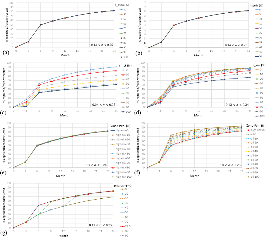
The first variable was r_asna. As explained in the Appendix, households’ ASNA indexes were predicted by a latent class regression model using household attributes. Then, the model assigned the predicted index to a household with a probability of r_asna% and assigned one of the other two indexes with a probability of (100 - r_asna)%. Therefore, this variable together with the household attributes affects the share of the population in each class, which in turn influences how the criterion on the recovery of the community will be satisfied. Figure 8 (a) illustrates the percentage of repaired/reconstructed houses (averaged on 100 runs) predicted on three-month intervals for different values of r_asna. The default value for the variable was 80%. The results suggest that the model is not sensitive to the changes in r_asna. However, insensitivity was caused by the input data, not the model structure. First, with the generated household attributes and assuming r_asna = 80%, about 65%, 31%, and 4% of the households were predicted to be of ASNA index 1, 2, and 3, respectively. Secondly, the rapid recovery of infrastructure caused the criterion on community recovery to be easily satisfied for index-1 households in the 3^rd month. Consequently, given the satisfaction of the financial criterion, there would be a good chance of repair/reconstruction for these households who meanwhile constitute a major share of the population. This also affects recovery decisions of the second largest part of the population (i.e., the index-2 (social-networks-aware) households). Since the community criterion for index-2 households is the adequate recovery of their neighbors, and many of the neighbors are of index 1 for which community criterion has already been satisfied, a high chance of repair/reconstruction once again exists for the index-2 households. Furthermore, although variation in the value of r_ansa changes the proportions of households, the dominant indexes are still 1 and 2. Therefore, the major shares of these classes combined with the fast recovery of infrastructure brought about the insensitivity of the model to changes in r_asna.

The next variable was r_prds. This variable identifies the random deviation of a household’s perceived neighborhood radius from the median radius corresponding to its ASNA index. For example, r_prds = 20% (default) means that for each household, the index-specific median radius is multiplied by a random draw from the interval 100±20 = [80, 120]% to yield the radius of its perceived neighborhood. Figure 8(b) suggests that the model is not sensitive to the changes in the value of r_prds. Since the community criterion for index-2 and index-3 households is evaluated on the recovery of neighbors and community assets that exist in the perceived neighborhood, changes in the radius of perceived neighborhoods alter their quantity and consequently affect the satisfaction of the criterion. However, the major share of index-1 households as neighbors of index-2 households and the small share of index-3 households caused the model not to show sensitivity to r_prds. Therefore, once again, this observation was produced by the input data and cannot be interpreted in general as the insensitivity of the model to r_prds.

Another variable was r_hbt. This variable identifies the threshold for the level of damage above which a house is assumed to be uninhabitable. The value of r_hbt impacts the model output in two aspects. First, it affects the amount of financial assistance that eligible households may receive from FEMA, as FEMA-HA is paid up to the amount of returning to the habitability level. Second, it determines whether households whose recovery criteria have not been satisfied can wait in their own house or must rent another residence (and if cannot, sell it). Figure 8(c) shows the sensitivity to r_hbt. The solid red line with triangular markers illustrates the output for the default value of r_hbt = 10%. The results show that the model is sensitive to this variable such that its smaller values speed up the progress of repair/reconstruction. The behavior corresponds to the output expected from the model algorithm. When r_hbt increases, the amount of FEAM-HA reimbursement decreases, which in turn causes the financial criterion not to be met for a higher number of households. Additionally, the increase in the value of this variable means that more households whose recovery criteria have not been met can wait in their own houses. Both consequences contributed to the overall decline in the progress of repair/reconstruction. Figure 8(c) further suggests that the model is almost insensitive to changes in r_hbt for values greater than 40%. This happened due to the level of damage estimated from tax assessment data. Based on this estimation, about 4% of damaged houses sustained a damage level greater than 40%, and only 1% were damaged by more than 50%. This share, however, was greater for lower levels of damage such that 64%, 39%, and 19% of houses burdened damage greater than 10%, 20%, and 30%, respectively. Therefore, since a few houses experienced damage greater than 40%, r_hbt above 40% did not affect the model output.

Sensitivity analysis was also performed on r_vac. This variable estimates the probability of availability of vacant rental units. If recovery criteria are not satisfied, the home is uninhabitable, and the household can afford to rent another residence, there is a probability of r_vac% that a vacant rental property, and consequently the option of waiting, would be available to the household. The results show that smaller values of the variable speed up the progress of repair/reconstruction. The change is less for smaller values of r_vac but increases with its growth such that changing r_vac from 0% to 50% decreases the percentage of repair/reconstruction in the 24^th month by about 1%, but changing the variable from 50% to 100% decreases the percentage by about 20%. This decrease is a result of the assumption of the model on decisions of households whose recovery criteria have not been met, their homes are uninhabitable and can afford to rent another residence. In such a case, most households prefer to wait (r₁ = 95%) rather than sell their property. Therefore, an increase in the value of r_vac means that more households will be able to wait in the hope of better conditions, which in turn results in a decrease in the overall percentage of repair/reconstruction, which could have happened after the sale. Oppositely, with a smaller r_vac, such households cannot find a place to rent and must sell their residence. A higher share of sold houses means that buyers, some of whom may decide to repair/reconstruct (r₀ = 35%), will have a higher share in the overall recovery. Although based on the model assumptions, a decrease in the availability of rental units would result in more repair/reconstruction, the extra amount is caused by new owners (buyers) at the cost of relocating the current households. Relocation is commonly deemed an unfavorable social phenomenon, as relocators may encounter problems in adapting to their new living environment, developing new social ties, and finding jobs which can trigger psychological burdens (Goenjian et al. 2001; Jamali et al. 2020; Najarian, Goenjian, Pelcovttz, Mandel, & Najarian 1996; Riad & Norris 1996; Uscher‐Pines 2009). Accordingly, motivating individuals to withstand deficiencies and rebuild instead of relocation is a near-consensus position among policymakers and researchers (Berke, Kartez, & Wenger 1993; Birkland 1997; Jamali et al. 2020; Kumar & Havey 2013). Therefore, the availability of rental units in the post-disaster setting is desirable, as it could help with reducing relocations and increasing households’ resilience and coping capacity (Cutter, Burton, & Emrich 2010; Moradi et al. 2019).

The next sensitivity analysis was implemented on the penetration of flood insurance. Based on the model algorithm, NFI settlements were the first type of financial resource assigned for repair/reconstruction. As described previously, it was assumed that 80% of households residing in high-risk flood zones benefited from flood insurance. Sensitivity analysis was performed to examine how changes in the default assumption impact the model outcome. For this purpose, it was first assumed that only high-risk zones may have insurance and the penetration rate changed from 50% to 100%. The results, as depicted in Figure 8(e), suggest that the overall outcome is not sensitive to variation in the insurance penetration rate. Again, this observation is rooted in the input data. RecovUS modeled 74,604 houses of which 42,645 houses were estimated to be damaged by Hurricane Sandy. However, a small number of them were located within the zones with a high risk of flooding (5,397 of total and 3,245 of the damaged houses). Consequently, considering the small share of damaged houses that potentially may have insurance (less than 8%), changes in the value of insurance penetration rate would not significantly alter the overall outcome. Therefore, in the second round of analyzing the sensitivity to the insurance penetration rate changes, eligible zones were expanded to the whole island. It was assumed that all zones may have insurance (regardless of the level of flood hazard), and the penetration rate varied from 10% to 100% (Figure 8(f)). The outcome shows that the model is sensitive to changes in the insurance penetration rate when it is applied to a sufficient number of houses. Insensitivity of the model when only high-risk zones are considered and its sensitivity once the region is expanded correspond to the reports that suspect accuracy and sufficiency of 100‐year flood maps as the boundaries of high-risk zones since a major share of losses happen outside of these boundaries (Brody et al. 2018; Highfield, Norman, & Brody 2013). Further, the model predicts that expanding the region to the whole island enhances the progress of repair/reconstruction even when a small penetration rate of 10% is applied. This outcome is also supported by the literature on the significant role of insurance in housing recovery and household resilience to disasters (Moradi et al. 2020; Nejat & Ghosh 2016; Tobin 1999). However, the model predicts that improvement in the amount of repair/reconstruction due to an increase in flood insurance penetration is more significant in the first few months and is diluted over time. For example, while the difference in the percentage of repair/reconstruction for penetration rates of 10% and 100% is about 22% in the 6^th month, it is lowered to 10% in the 24^th month. This means that while a higher penetration accelerates the progress of repair/reconstruction and speeds up the return to normalcy, it might not significantly change the long-term outcome. Meanwhile, considering the controversial aspects of the National Flood Insurance Program such as recognizing improper land development, mitigation failures, and actuarial unsoundness (Burby 2001; Kunreuther 1996; McMillan 2007), the decision for increasing insurance penetration requires more consideration.

Finally, the sensitivity to different regimes of infrastructure recovery was evaluated. As described before, it was estimated that infrastructure majorly recovered in the first three months (77.5%) and completely recovered by the end of the 6^th month. To examine the influence of different recovery regimes, the three-month rate of infrastructure recovery changed from 0% to 90% (Figure 9), and the predicted progress in housing repair/reconstruction was compared (Figure 8(g)).

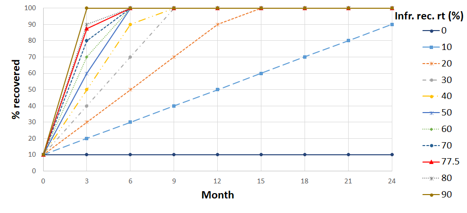
Figure 8(g) shows four patterns for housing repair/reconstruction based on different values for infrastructure recovery rate: a pattern for an infrastructure recovery rate of 0%, a pattern for 10%, a pattern for 20% and 30%, and a pattern for 40% to 90%. The outcome suggests that quicker infrastructure recovery results in an enhancement in the progress of housing repair/reconstruction in months 3-15. This improvement is caused due to satisfaction of the community criterion for index-1 households and its ripple effect on the recovery of index-2 households, which together constitute about 96% of the households. This observation is aligned with the literature that reports the positive effect of infrastructure functionality on housing repair/reconstruction (Arup 2016; Burton 2015; Comerio 2014; Miles & Chang 2011; Moradi et al. 2019).

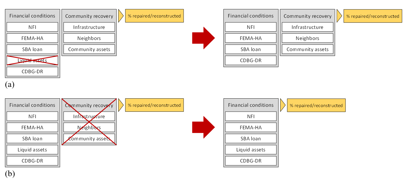
The sensitivity analyses presented above rely on a local technique in which variables are changed one at a time. When a model includes nonlinearities and interactions, a global sensitivity analysis is also necessary since local methods do not adequately represent its sensitivity (Saltelli et al. 2019). In this research, an ablation study was performed to evaluate the global sensitivity of the model. Ablation study examines a model by removing its building blocks to examine their effect on the model output (Hessel et al. 2018; Meyes et al. 2019; Sheikholeslami 2019). As described previously, RecovUS is based on two fundamental assumptions stating that financial conditions and community recovery are the prerequisites for housing repair/reconstruction. Each of these assumptions includes several blocks; financial conditions consist of five blocks of NFI, FEMA-HA, SBA loan, liquid assets, and CDBG-DR, and community recovery includes three blocks of recovery of infrastructure, neighbors, and community assets. To examine the effect of each block on the overall repair/reconstruction of households, the model was run with excluding the block from the algorithm. For example, the effect of liquid assets on the percentage of repair/reconstruction was evaluated by removing the block of liquid assets. In other words, it was assumed that households would not spend any share of their liquid assets on repair/reconstruction (Figure 10 (a)), the model was run 100 times, and the results were averaged. Additionally, the effect of each fundamental assumption was evaluated by removing all of its constituent blocks. Figure 10 (b) schematically shows removing the fundamental assumption of community recovery as an example. The analysis results are illustrated in Figure 11.

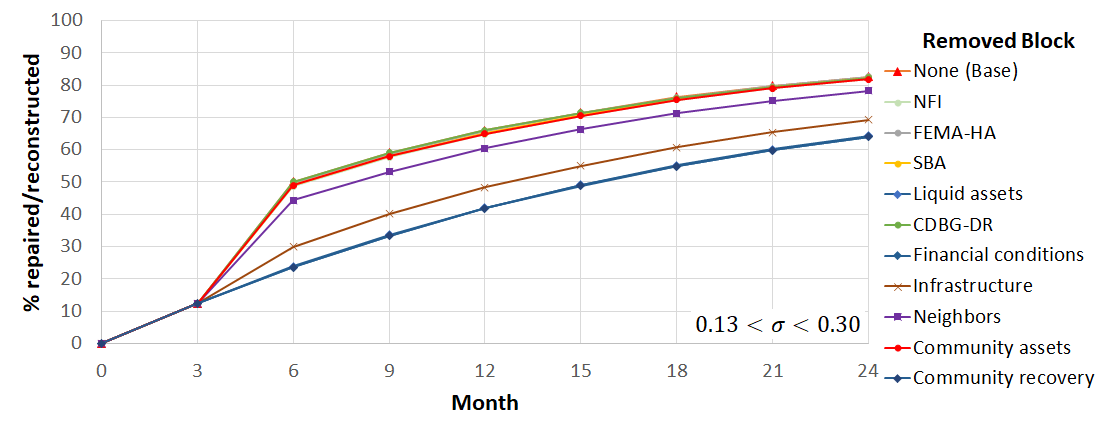
Four distinctive patterns are observed in Figure 11. The highest ratio of repair/reconstruction is achieved in the base case in which none of the blocks are removed. Removing NFI, FEMA-HA, SBA loan, CDBG-DR assistance, and recovery of community assets does not change this pattern significantly. With the input data and assumptions described before, the share of NFI, FEMA-HA, SBA loan, and CDBG-DR assistance from the total financial resources available to households for repair/reconstruction was about 8%, 4%, 7%, and 10% respectively. Therefore, each of these resources could not individually affect the overall outcome much. However, although it might be argued that the mentioned resources were not shown to greatly influence the recovery of the community, it should be noted that each of them is important to their eligible population. For example, CGBG-DR assistance is mainly intended to help with the recovery of lower-income households. Therefore, although it constituted only 10% of the total resources and slightly influenced the global pattern of recovery, it helped with recovery of a particular portion of the population who could not afford the cost of repair/reconstruction without this type of assistance. The insensitivity of the model to the recovery of community assets also resulted from the small share of community-assets-aware households (less than 5%) studied in this research. In the current study, recovery of community assets did not help much with the overall recovery of households; however, they are still important to the recovery of different communities where a higher share of households perceive community assets as the most important anchors of their neighborhood.

On the other hand, removing the block of liquid assets, the assumption of financial conditions, or the assumption of community recovery results in the largest decline in the overall ratio of repair/reconstruction. Liquid assets constituted more than two-thirds of the financial resources. Consequently, removing this resource affected the overall outcome like the case in which financial conditions were not satisfied at all. Interestingly, removing the assumption of community recovery as a recovery criterion impacted the overall repair/reconstruction of households similar to removing the assumption of satisfaction of financial conditions. This result suggests that the two fundamental assumptions of this study (i.e., availability of financial resources and restoration of perceived community) are equally important to homeowners’ recovery decisions.

Two other curves exist between these two extremes: removing the block of recovery of neighbors and restoration of infrastructure. By removing the block of recovery of neighbors, social-network-aware households will perceive that their neighborhood has not recovered at all. Removing the block of recovery of infrastructure has a similar meaning to the infrastructure-aware households. Figure 11 shows that the effect of infrastructure restoration on the overall recovery of households is more than the neighbors’ recovery. This is because first, the number of infrastructure-aware households in this study was twice the number of social-network-aware households (about two-thirds and one-third of the households, respectively). Second, the non-functionality of infrastructure not only directly impacts the repair/reconstruction decision of infrastructure-aware households but also indirectly affects recovery decisions of social-network-aware households since most of their neighbors are infrastructure-aware. Therefore, recovery of infrastructure had a ripple effect on the recovery of households.

The experiments explained above helped with addressing the research objectives. The results showed that internal, interactive, and external drivers of recovery affected households’ recovery decisions. As described before (Figure 5), the model incorporated three categories of drivers: internal (household income, education, and race, and physical damage), interactive (recovery of perceived neighbors), and external (financial assistance, recovery of infrastructure, and recovery of community assets). Household income, education, and race are the internal drivers that estimate a household’s ASNA index. This index classifies households based on their perception of the community, which in turn identifies the share of recovery of infrastructure, neighbors, and community assets in households’ decisions. Most households were estimated to be infrastructure aware (about 65%). The second major group was social-networks-aware households (about 30%) for which recovery of community assets mattered most. The last class (i.e., community-assets-aware households) constituted a minor share of households (less than 5%). Accordingly, recovery of infrastructure followed by recovery of neighbors had the highest impact on the recovery of households. It is worth noting that recovery of infrastructure has a ripple effect since it directly impacts infrastructure-aware households and indirectly affects social-networks-aware households (through their infrastructure-aware neighbors), which together constitute about 96% of the households. This relationship is observed in Figure 8(g) as the higher rates of infrastructure recovery are associated with accelerated progress in households’ repairs/reconstructions. This positive relationship has been reported in the literature as described before (Comerio 2014; Nejat & Damnjanovic 2012; Xiao et al. 2018). Damage to houses is also an important driver, as it identifies whether a household can afford the cost of repair/reconstruction. More severe damage requires more financial resources and is often associated with lower odds of repair/reconstruction (Mayer et al. 2020; McNeil et al. 2015). Additionally, the impact of financial resources is reflected in Figure 8(c) and (f). Increasing the amount of financial aid (e.g., increasing FEMA-HA reimbursement through decreasing r_hbt) and expanding the aid to accommodate more households (e.g., increasing insurance penetration rate) enhance the progress of repair/reconstruction. This observation is also supported by the literature (Kamel & Loukaitou-Sideris 2004; Nejat & Ghosh 2016; Tobin 1999). Therefore, seven out of the eight drivers of recovery employed in the model effectively impacted the recovery of households. Recovery of community assets had a relatively small share due to the small number of households indexed as community-assets aware. Additionally, the results showed that the fundamental assumptions of the study (i.e., availability of financial resources and recovery of perceived community), both are important to homeowners’ recovery decisions and affect the overall pattern of repair/reconstruction to a similar degree (Figure 11). Among constituents of the first assumption, liquid assets had the highest impact due to its major share in financial resources. Among the elements of the second assumption, restoration of infrastructure followed by recovery of community assets played the key role because most households were indexed as infrastructure-aware and social-network-aware.

Conclusions

This research aims to develop a model that could integrate the effects of financial resources and communal aspects of recovery by capturing spatial interactions of households with their perceived neighborhood. While several models have been proposed for the simulation of recovery, the major contribution of this research is to develop a model that simulates housing decisions through the mindset of insiders. In RecovUS, not only do factors such as level of damage, financial resources, and affordability and availability of rental properties affect households’ decisions in favor of repair/reconstruction, waiting, or selling, but also their perception of their neighborhood and its restoration also play a critical role. The model separates this perception for different residents such that heterogeneous households prefer community features dissimilar in terms of type and distance. The output from the model confirms that internal, interactive, and external drivers of recovery effectively play a role in the households’ decision-making and influence the progress of repair/reconstruction. Therefore, RecovUS contributes to the field of disaster recovery modeling by weighting the communal aspects of recovery and calling out the necessity of including households’ interactions with their perceived neighborhood for achieving a more realistic simulation and prediction.

Like all studies, the current research was associated with limitations. Addressing these limitations could be future lines of study. A challenge was providing individual-level data on damage and restoration of properties. Although this information was estimated from tax assessment data, the approach comes with a limitation: properties are appraised within a fiscal year, not on a single date. Therefore, based on the time that a disaster impacts a region and the date on which a property is appraised, the value may be related to the status of a house in 1 to 364 days after the disaster. This influences estimation of both damage and repair/reconstruction. Although discounting all values back to a base date helped with alleviating market inflations and comparability of the values, the estimation is still affected by the recovery stage on which a building has been appraised. Moreover, the value of a building can be affected by a variety of causes other than physical damage such as market dynamics, depreciation, upgrade, etc. However, in the spatiotemporal vicinity of a disaster (like the case studied in this research), the price changes can be plausibly assumed to be caused by the physical damage and the restoration progress, though there still might be inaccuracies. Damage could be estimated using other methods and applied to evaluate the expected capability of the model in simulating different patterns.

Also, the model does not impose any time limit on the duration of renting. Households that afford the rent and can find a vacant unit may wait up to the last run of the program (24 months). However, although temporary housing may take weeks to months (Peacock et al. 2007), it is not necessarily via renting a place. For at least the first few months, many higher-income households may decide to stay at hotels and motels, while lower income households may stay with their friends and families (Morrow & Peacock 1997; Peacock et al. 2007). However, the model assumes they will rent. Additionally, the model does not include programs that facilitate temporary housing by providing cash rental assistance, mobile homes, etc. These subjects can be accommodated in future research.

Furthermore, although RecovUS neither underfits nor overfits the data, the generalization of the model to other disaster scenarios needs additional consideration. For example, the spatial pattern of damage is different in a hurricane or earthquake from a tornado. While hurricanes typically affect a vast area, tornadoes usually have a local spatial expansion and impact a limited region on and around their path. In addition to the type of disaster, other factors such as characteristics of households, types and timing of financial resources, and recovery of infrastructure and community assets can be significantly different. When input data is much different, the parameters should be optimized by recalibrating the model, while some submodules may even require modification. Such data can help with evaluating the generalizability of the model to other types of disasters, different socioeconomic structures, various distributions of financial resources, and different patterns in the restoration of infrastructure and community assets.

The model development was also influenced by technical constraints. Due to the software and HPCC limitations, the number of model parameters was restricted to reduce the calibration duration. Consequently, RecovUS was calibrated on six variables. In the absence of this limitation, more parameters could have been employed to accommodate different conditions. For example, the probability of selecting the wait option, conditioned on whether a home is habitable or not, could be represented by two different parameters, rather than by a single parameter (r₁) as is in the current version. Moreover, RecovUS was calibrated by minimizing the disagreement between the predicted and observed outcomes (i.e., recovery decisions). While percent agreement is a commonly used method, calibrating the model using other measures such as the kappa statistic could decrease the potential of chance agreement. Additionally, aggregating the household-level results into a larger geographical unit (e.g. block group) can provide additional insights into the spatial nature of recovery decisions.

Another important subject is the possible loss of income due to the collapse of the local economy. In the current study, household-level income was estimated from the 2013 census data and was used to estimate households’ ASNA indexes, rent power, net worth, and eligibility for SBA loan and CDBG-DR assistance. Although the changes in household income are expected to have been reflected in the American Community Survey estimates, it still might affect the income-related values. The potential effect of income variability can be integrated into future versions of the model.

Finally, the current research examined homeowners’ recovery decisions residing in their primary single-family detached houses. More research is required to study the recovery of other types of occupancy and housing characteristics. Recovery of renters, secondary homes, multifamily properties, etc. are important subjects that require more study. Therefore, expanding the model to include other aspects of recovery can be the subject of another study.

Despite the limitations, RecovUS provides a platform to spatially model houses and community assets to examine the impacts of financial aids and restoration of community on recovery decisions of households with heterogeneous characteristics. RecovUS benefits from the advantage of calibration and modular structure. If assumptions or input data are to be included that are significantly different from the current research, the model can be recalibrated to optimize its parameters or, if required, submodules can be easily modified to address the new conditions without impacting the model’s integrity. For example, this study assumed that households whose recovery criteria have not been met may wait for the whole runtime (i.e., 24 months), if their home is habitable or they are able to rent another place. Other options, such as staying with friends and families rather than renting, staying with significant others in the first few months and then renting another place, substituting the wait/sell parameter with time-sensitive parameters such that the weight of the sell option increases over time, etc. are of possible modifications that could be easily incorporated into the model. New submodules can also be added (e.g., to simulate business recovery), while the integrity of the model stays preserved.

Another feature of RecovUS is that the required input can be obtained from free and publicly available data sources. The idea behind this design was to provide a model that could offer a perspective toward the situation at a minimum amount of time and cost. Additionally, if more specific and accurate data is provided, the model could be easily fine-tuned. Therefore, RecovUS can help with data-driven planning by providing a tool for predicting impacts of different resource allocation and reconstruction scenarios to outline policies that could better address social, economic, and political concerns while accommodating the various needs of different stakeholders.

References

AGHABABAEI, M., Koliou, M., Watson, M., & Xiao, Y. (2020). Quantifying post-disaster business recovery through Bayesian methods. Structure and Infrastructure Engineering , 1-19. [doi:10.1080/15732479.2020.1777569]

AIRRIESS, C. A., Li, W., Leong, K. J., Chen, A. C. C., & Keith, V. M. (2008). Church-based social capital, networks and geographical scale: Katrina evacuation, relocation, and recovery in a New Orleans Vietnamese American community. Geoforum, 39(3), 1333-1346. [doi:10.1016/j.geoforum.2007.11.003]

ALDRICH, D. P. (2010). Fixing recovery: Social capital in post-crisis resilience. Journal of Homeland Security, 6, 1-10.

ALDRICH, D. P. (2011). The power of people: Social capital’s role in recovery from the 1995 Kobe earthquake. Natural Hazards, 56(3), 595-611. [doi:10.1007/s11069-010-9577-7]

ARUP. (2016). City Resilience Index - Inside the CRI: Reference guide. Retrieved from London, UK: https://www.alnap.org/help-library/inside-the-cri-reference-guide.

BERGHOLT, D., & Lujala, P. (2012). Climate-related natural disasters, economic growth, and armed civil conflict. Journal of Peace Research, 49(1), 147-162. [doi:10.1177/0022343311426167]

BERKE, P. R., Kartez, J., & Wenger, D. (1993). Recovery after disaster: achieving sustainable development, mitigation and equity. Disasters, 17(2), 93-109. [doi:10.1111/j.1467-7717.1993.tb01137.x]

BINDER, S. B., Baker, C. K., & Barile, J. P. (2015). Rebuild or relocate? Resilience and postdisaster decision-making after Hurricane Sandy. American Journal of Community Psychology, 56(1-2), 180-196. [doi:10.1007/s10464-015-9727-x]

BIRKLAND, T. A. (1997). After Disaster: Agenda Setting, Public Policy, and Focusing Events: Georgetown University Press.

BLS. (2019). Housing in New York-Newark-Jersey City.

BRATT, R. G. (2002). Housing and family well-being. Housing Studies, 17(1), 13-26. [doi:10.1080/02673030120105857]

BRODY, S., Sebastian, A., Blessing, R., & Bedient, P. (2018). Case study results from southeast Houston, Texas: identifying the impacts of residential location on flood risk and loss. Journal of Flood Risk Management, 11, S110-S120. [doi:10.1111/jfr3.12184]

BULLARD, R. D., & Wright, B. (2009). Race, Place, and Environmental Justice after Hurricane Katrina: Struggles to Reclaim, Rebuild, and Revitalize New Orleans and the Gulf Coast. Boulder: Westview Press. [doi:10.4324/9780429497858-1]

BURBY, R. J. (2001). Flood insurance and floodplain management: the US experience. Global Environmental Change Part B: Environmental Hazards, 3(3), 111-122. [doi:10.1016/s1464-2867(02)00003-7]

BURTON, C. G. (2015). A validation of metrics for community resilience to natural hazards and disasters using the recovery from Hurricane Katrina as a case study. Annals of the Association of American Geographers, 105(1), 67-86. [doi:10.1080/00045608.2014.960039]

CAMPBELL, E., Henly, J. R., Elliott, D. S., & Irwin, K. (2009). Subjective constructions of neighborhood boundaries: Lessons from a qualitative study of four neighborhoods. Journal of Urban Affairs, 31(4), 461-490. [doi:10.1111/j.1467-9906.2009.00450.x]

COMERIO, M. C. (1998). Disaster Hits Home: New Policy for Urban Housing Recovery. Berkeley, CA: University of California Press.

COMERIO, M. C. (2014). Disaster recovery and community renewal: Housing approaches. Cityscape, 16(2), 51-64.

COULTON, C. J., Jennings, M. Z., & Chan, T. (2013). How big is my neighborhood? Individual and contextual effects on perceptions of neighborhood scale. American Journal of Community Psychology, 51(1-2), 140-150. [doi:10.1007/s10464-012-9550-6]

COULTON, C. J., Korbin, J., Chan, T., & Su, M. (2001). Mapping residents' perceptions of neighborhood boundaries: a methodological note. American Journal of Community Psychology, 29(2), 371-383. [doi:10.1023/a:1010303419034]

CUTTER, S. L., Barnes, L., Berry, M., Burton, C., Evans, E., Tate, E., & Webb, J. (2008). A place-based model for understanding community resilience to natural disasters. Global Environmental Change, 18(4), 598-606. [doi:10.1016/j.gloenvcha.2008.07.013]

CUTTER, S. L., Burton, C. G., & Emrich, C. T. (2010). Disaster resilience indicators for benchmarking baseline conditions. Journal of Homeland Security and Emergency Management, 7(1), 1-22. [doi:10.2202/1547-7355.1732]

DE Koning, K., & Filatova, T. (2020). Repetitive floods intensify outmigration and climate gentrification in coastal cities. Environmental Research Letters, 15(3), 034008. [doi:10.1088/1748-9326/ab6668]

DEHGHANI, N. L., & Shafieezadeh, A. (2019). Probabilistic sustainability assessment of bridges subjected to multi-occurrence hazards. Paper presented at the International Conference on Sustainable Infrastructure 2019: Leading Resilient Communities through the 21st Century. [doi:10.1061/9780784482650.059]

DRABEK, T. E. (2012). Human System Responses to Disaster: An Inventory of Sociological Findings. Berlin Heidelberg: Springer Science & Business Media.

ESRI. (2015). ArcGIS Desktop Release 10.3.1. Redlands, CA: Environmental Systems Research Institute (ESRI).

FEMA. (2011). National disaster recovery framework - Strengthening disaster recovery for the nation. Retrieved from https://www.fema.gov/pdf/recoveryframework/ndrf.pdfFEMA. (2019a) (03/18/2019). Flood zones. Retrieved from https://www.fema.gov/flood-zones.

FEMA. (2019b). OpenFEMA dataset: Housing assistance data owners - V1. Retrieved Sep. 19, 2019, from The Federal Emergency Management Agency (FEMA) https://www.fema.gov/media-library-data/1510759434562-dfb20c9a88200a9b6eae4a8e26443b75/FactSheet_Flooding_Am_I_At_Risk.pdf.

FILATOVA, T., Parker, D. C., & van der Veen, A. (2011). The implications of skewed risk perception for a Dutch coastal land market: insights from an agent-based computational economics model. Agricultural and Resource Economics Review, 40(3), 405-423. [doi:10.1017/s1068280500002860]

FRBNY. (2018). Quarterly report on household debt and credit. Retrieved from: https://www.newyorkfed.org/microeconomics/hhdc.html.

GANAPATI, N. E., & Ganapati, S. (2008). Enabling participatory planning after disasters: A case study of the World Bank's housing reconstruction in Turkey. Journal of the American Planning Association, 75(1), 41-59. [doi:10.1080/01944360802546254]

GAO. (2015). Hurricane Sandy: An Investment Strategy Could Help the Federal Government Enhance National Resilience for Future Disasters. Retrieved from: https://www.gao.gov/products/GAO-15-515.

GOENJIAN, A. K., Molina, L., Steinberg, A. M., Fairbanks, L. A., Alvarez, M. L., Goenjian, H. A., & Pynoos, R. S. (2001). Posttraumatic stress and depressive reactions among Nicaraguan adolescents after Hurricane Mitch. American Journal of Psychiatry, 158(5), 788-794. [doi:10.1176/appi.ajp.158.5.788]

GOODFELLOW, I., Bengio, Y., & Courville, A. (2016). Deep Learning. Cambridge, Massachusetts: The MIT Press.

GRIMM, V., Berger, U., Bastiansen, F., Eliassen, S., Ginot, V., Giske, J., . . . Huse, G. (2006). A standard protocol for describing individual-based and agent-based models. Ecological Modelling, 198(1-2), 115-126. [doi:10.1016/j.ecolmodel.2006.04.023]

GRIMM, V., Railsback, S. F., Vincenot, C. E., Berger, U., Gallagher, C., DeAngelis, D. L., . . . Groeneveld, J. r. (2020). The odd protocol for describing agent-based and other simulation models: A second update to improve clarity, replication, and structural realism. Journal of Artificial Societies and Social Simulation, 23(2), 7: https://www.jasss.org/23/2/7.html. [doi:10.18564/jasss.4259]

GUHA-SAPIR, D., Hoyois, P., & Below, R. (2016). Annual disaster statistical review 2015: The numbers and trends. Retrieved from Brussels: https://reliefweb.int/report/world/annual-disaster-statistical-review-2015-numbers-and-trends.

HAER, T., Botzen, W. W., & Aerts, J. C. (2016). The effectiveness of flood risk communication strategies and the influence of social networks—Insights from an agent-based model. Environmental Science & Policy, 60, 44-52. [doi:10.1016/j.envsci.2016.03.006]

HAMIDEH, S., Peacock, W. G., & Zandt, S. V. (2018). Housing Recovery after Disasters: Primary versus Seasonal and Vacation Housing Markets in Coastal Communities. Natural Hazards Review, 19(2), 04018003. [doi:10.1061/(asce)nh.1527-6996.0000287]

HANEY, W. G., & Knowles, E. S. (1978). Perception of neighborhoods by city and suburban residents. Human Ecology, 6(2), 201-214. [doi:10.1007/bf00889095]

HENDERSON, T. L., Roberto, K. A., & Kamo, Y. (2010). Older adults' responses to Hurricane Katrina daily hassles and coping strategies. Journal of Applied Gerontology, 29(1), 48-69. [doi:10.1177/0733464809334287]

HESSEL, M., Modayil, J., Van Hasselt, H., Schaul, T., Ostrovski, G., Dabney, W., . . . Silver, D. (2018). Rainbow: Combining improvements in deep reinforcement learning. Paper presented at the Thirty-Second AAAI Conference on Artificial Intelligence.

HIGHFIELD, W. E., Norman, S. A., & Brody, S. D. (2013). Examining the 100‐year floodplain as a metric of risk, loss, and household adjustment. Risk Analysis: An International Journal, 33(2), 186-191. [doi:10.1111/j.1539-6924.2012.01840.x]

HIRAYAMA, Y. (2000). Collapse and reconstruction: Housing recovery policy in Kobe after the Hanshin Great Earthquake. Journal of Housing Studies, 15(1), 111-128. [doi:10.1080/02673030082504]

HPCC. (2019). High Performance Computing Center.

HRD (Producer). (2019). Hurricane Research Division: The thirty costliest mainland United States tropical cyclones 1900-2013. Retrieved from http://www.aoml.noaa.gov/hrd/tcfaq/costliesttable.html.

HUD. (2019). Fair Market Rents. Retrieved Sep. 22, 2019, from The United States Department of Housing and Urban (HUD): https://www.huduser.gov/portal/datasets/fmr.html.

HUNTER, L. M. (2005). Migration and environmental hazards. Population and Environment, 26(4), 273-302.

III. (2019a). Facts + Statistics: Flood insurance. Retrieved from https://www.iii.org/fact-statistic/facts-statistics-flood-insurance.

III. (2019b). Facts + Statistics: Hurricanes. Retrieved from https://www.iii.org/fact-statistic/facts-statistics-hurricanes.

INGRAM, J. C., Franco, G., Rumbaitis-del Rio, C., & Khazai, B. (2006). Post-disaster recovery dilemmas: challenges in balancing short-term and long-term needs for vulnerability reduction. Environmental Science & Policy, 9(7-8), 607-613. [doi:10.1016/j.envsci.2006.07.006]

JAMALI, M., & Nejat, A. (2016). Place attachment and disasters: Knowns and unknowns. Journal of Emergency Management, 14(5), 349-364.

JAMALI, M., Nejat, A., Moradi, S., Ghosh, S., Jin, F., & Cao, G. (2020). Social media data and housing recovery following extreme natural events. International Journal of Disaster Risk Reduction, 51. [doi:10.1016/j.ijdrr.2020.101788]

KAMEL, N. M., & Loukaitou-Sideris, A. (2004). Residential assistance and recovery following the Northridge earthquake. Urban Studies, 41(3), 533-562. [doi:10.1080/0042098042000178672]

KAUFMAN, C., & Shaby, B. (2013). The role of the range parameter for estimation and prediction in geostatistics. Biometrika, 100(2), 473-484. [doi:10.1093/biomet/ass079]

KRYSAN, M. (2002). Community undesirability in black and white: Examining racial residential preferences through community perceptions. Social Problems, 49(4), 521-543. [doi:10.1525/sp.2002.49.4.521]

KUMAR, S., & Havey, T. (2013). Before and after disaster strikes: A relief supply chain decision support framework. International Journal of Production Economics, 145(2), 613-629. [doi:10.1016/j.ijpe.2013.05.016]

KUNREUTHER, H. (1996). Mitigating disaster losses through insurance. Journal of risk and Uncertainty, 12(2-3), 171-187. [doi:10.1007/bf00055792]

MAGLIOCCA, N., Safirova, E., McConnell, V., & Walls, M. (2011). An economic agent-based model of coupled housing and land markets (CHALMS). Computers, Environment and Urban Systems, 35(3), 183-191. [doi:10.1016/j.compenvurbsys.2011.01.002]

MAGLIOCCA, N. R., & Walls, M. (2018). The role of subjective risk perceptions in shaping coastal development dynamics. Computers, Environment and Urban Systems, 71, 1-13. [doi:10.1016/j.compenvurbsys.2018.03.009]

MAYER, J., Moradi, S., Nejat, A., Ghosh, S., Cong, Z., & Liang, D. (2020). Drivers of post-disaster relocations: The case of Moore and Hattiesburg tornados. International Journal of Disaster Risk Reduction, 101643. [doi:10.1016/j.ijdrr.2020.101643]

MCMILLAN, C. M. (2007). Federal Flood Insurance Policy: Making Matters Worse. Houston Law Review, 44, 471.

MCNEIL, S., Mininger, K., Greer, A., & Trainor, J. (2015). Household residential decision-making in the wake of disaster: Report of results prepared for sea bright residents. Disaster Research Center.

MEYES, R., Lu, M., de Puiseau, C. W., & Meisen, T. (2019). Ablation studies in artificial neural networks. arXiv preprint arXiv:1901.08644.

MILES, S. B. (2017). DESaster: A discrete event disaster recovery simulation built on top of the Simpy discrete event simulation Python library. Retrieved from https://github.com/milessb/DESaster.

MILES, S. B., & Chang, S. E. (2006). Modeling community recovery from earthquakes. Earthquake Spectra, 22(2), 439-458. [doi:10.1193/1.2192847]

MILES, S. B., & Chang, S. E. (2011). ResilUS: A community based disaster resilience model. Cartography and Geographic Information Science, 38(1), 36-51. [doi:10.1559/1523040638136]

MORADI, S. (2020a). RecovUS: An agent-based model of post-disaster household recovery (Version 1.0.0). https://www.comses.net/codebases/8f1d300e-6333-4b36-820f-c414016ea395/releases/1.0.0/: CoMSES Computational Model Library.

MORADI, S. (2020b). RecovUS: An Agent-Based Model of Post-Disaster Housing Recovery. (Ph.D.), Texas Tech University, Lubbock, TX.

MORADI, S., Nejat, A., Hu, D., & Ghosh, S. (2020). Perceived neighborhood: Preferences versus actualities. International Journal of Disaster Risk Reduction, 51, 101824. [doi:10.1016/j.ijdrr.2020.101824]

MORADI, S., Vasandani, V., & Nejat, A. (2019). A review of resilience variables in the context of disasters. Journal of Emergency Management, 17(5), 403-432.

MORROW, B. H., & Peacock, W. G. (1997). 'Disasters and social change: Hurricane Andrew and the reshaping of Miami.' In Peacock, W. G. & Gladwin, H. (Eds.), Hurricane Andrew: Ethnicity, Gender and the Sociology of Disasters. London: Routledge, pp. 226-242.

MYERS, C. A., Slack, T., & Singelmann, J. (2008). Social vulnerability and migration in the wake of disaster: The case of Hurricanes Katrina and Rita. Population and Environment, 29(6), 271-291. [doi:10.1007/s11111-008-0072-y]

NAJARIAN, L. M., Goenjian, A. K., Pelcovttz, D., Mandel, F., & Najarian, B. (1996). Relocation after a disaster: Posttraumatic stress disorder in Armenia after the earthquake. Journal of the American Academy of Child & Adolescent Psychiatry, 35(3), 374-383. [doi:10.1097/00004583-199603000-00020]

NAZARNIA, H., Sarmasti, H., & Wills, W. O. (2020). Application of household disruption data to delineate critical infrastructure resilience characteristics in the aftermath of disaster: A case study of Bhaktapur, Nepal. Safety Science, 121, 573-579. [doi:10.1016/j.ssci.2019.02.014]

NEJAT, A. (2018). Perceived neighborhood boundaries: A missing link in modeling post-disaster housing recovery. International Journal of Disaster Risk Reduction, 28, 225-236. [doi:10.1016/j.ijdrr.2017.12.001]

NEJAT, A., Binder, S. B., Greer, A., & Jamali, M. (2018). Demographics and the dynamics of recovery: A latent class analysis of disaster recovery priorities after the 2013 Moore, Oklahoma tornado. International Journal of Mass Emergencies & Disasters, 36(1), 23-51.

NEJAT, A., & Damnjanovic, I. (2012). Agent-based modeling of behavioral housing recovery following disasters. Computer-Aided Civil and Infrastructure Engineering, 27(10), 748-763. [doi:10.1111/j.1467-8667.2012.00787.x]

NEJAT, A., & Ghosh, S. (2016). LASSO model of postdisaster housing recovery: Case study of Hurricane Sandy. Natural Hazards Review, 17(3), 04016007. [doi:10.1061/(asce)nh.1527-6996.0000223]

NEJAT, A., Javid, R. J., Ghosh, S., & Moradi, S. (2020). A spatially explicit model of postdisaster housing recovery. Computer-Aided Civil and Infrastructure Engineering, 35(2), 150-161. [doi:10.1111/mice.12487]

NEJAT, A., Moradi, S., & Ghosh, S. (2019). Anchors of social network awareness index: A key to modeling postdisaster housing recovery. Journal of Infrastructure Systems, 25(2), 04019004. [doi:10.1061/(asce)is.1943-555x.0000471]

NOAA, & NWS. (2013). Hurricane/Post-Tropical Cyclone Sandy: Service Assessment. Retrieved from: https://www.weather.gov/media/publications/assessments/Sandy13.pdf.

NYC. (2013). A stronger, more resilient New York. Retrieved from: https://www1.nyc.gov/site/sirr/report/report.page.

NYC. (2019a). Assessments.

NYC. (2019b). Department of Finance Digital Tax Map.

NYC. (2019c). Sandy funding tracker. Retrieved Sep. 27, 2019

PEACOCK, W. G., Dash, N., & Zhang, Y. (2007). 'Sheltering and Housing Recovery Following Disaster.' In H. Kaplan (Ed.), Handbook of Disaster Research. New York, NY: Springer, pp. 258-274. [doi:10.1007/978-0-387-32353-4_15]

PEACOCK, W. G., Van Zandt, S., Zhang, Y., & Highfield, W. E. (2014). Inequities in long-term housing recovery after disasters. Journal of the American Planning Association, 80(4), 356-371. [doi:10.1080/01944363.2014.980440]

POLSKY, C. (2019, March 3, 2019). A third of homes auctioned by NY Rising have been redeveloped. Retrieved from https://www.newsday.com/long-island/new-york-rising-auction-1.27929847-.

PRAVETTONI, R. (2009). Number of disasters per year. GRID-Arendal.

RIAD, J. K., & Norris, F. H. (1996). The influence of relocation on the environmental, social, and psychological stress experienced by disaster victims. Environment and Behavior, 28(2), 163-182. [doi:10.1177/0013916596282001]

RONAN, K., & Johnston, D. (2005). Promoting Community Resilience in Disasters: The Role for Schools, Youth, and Families. New York: Springer Science & Business Media. [doi:10.1007/b102725]

RUBIN, C. B. (2009). Long term recovery from disasters - The neglected component of emergency management. Journal of Homeland Security and Emergency Management, 6(1). [doi:10.2202/1547-7355.1616]

RUST, E. B., & Killinger, K. (2006). The financial services roundtable blue ribbon commission on mega-catastrophes: A call to action. Washington, DC: Financial Services Roundtable.

SADRI, A. M., Ukkusuri, S. V., Lee, S., Clawson, R., Aldrich, D., Nelson, M. S., . . . Kelly, D. (2018). The role of social capital, personal networks, and emergency responders in post-disaster recovery and resilience: a study of rural communities in Indiana. Natural Hazards, 90(3), 1377-1406. [doi:10.1007/s11069-017-3103-0]

SALTELLI, A., Aleksankina, K., Becker, W., Fennell, P., Ferretti, F., Holst, N., . . . Wu, Q. (2019). Why so many published sensitivity analyses are false: A systematic review of sensitivity analysis practices. Environmental Modelling & Software, 114, 29-39. [doi:10.1016/j.envsoft.2019.01.012]

SANDERS, S., Bowie, S. L., & Bowie, Y. D. (2004). Chapter 2 Lessons Learned on Forced Relocation of Older Adults: The Impact of Hurricane Andrew on Health, Mental Health, and Social Support of Public Housing Residents. Journal of Gerontological Social Work, 40(4), 23-35. [doi:10.1300/j083v40n04_03]

SBA. (2014). SBA disaster loan data superstorm Sandy. Retrieved Sep. 27, 2019, from The United States Small Business Administration (SBA) https://www.sba.gov/funding-programs/disaster-assistance.

SCHWARTZ, E. (2006). A needless toll of natural disasters. Boston Globe. 3/23/: https://reliefweb.int/report/philippines/needless-toll-natural-disasters.

SHAWNEE County. (2019). Definitions of FEMA flood zone designations. In. http://snmapmod.snco.us/fmm/document/fema-flood-zone-definitions.pdf.

SHEIKHOLESLAMI, S. (2019). Ablation Programming for Machine Learning. M.Sc. Thesis, KTH Royal Institute of Technology.

SMITH, G. (2012). Planning for Post-Disaster Recovery: A Review of the United States Disaster Assistance Framework. Washington, DC: Island Press.

THEODORIDIS, S. (2015). Machine Learning: A Bayesian and Optimization Perspective. London, UK: Academic Press.

TOBIN, G. A. (1999). Sustainability and community resilience: The holy grail of hazards planning? Global Environmental Change Part B: Environmental Hazards, 1(1), 13-25. [doi:10.1016/s1464-2867(99)00002-9]

TWOMEY, J. M., & Smith, A. E. (1997). 'Validation and verification.' In N. Kartam, I. Flood, & J. Garrett (Eds.), Artificial Neural Networks for Civil Engineers: Fundamentals and Applications. New York, NY: ASCE Press, pp. 44-64.

USCB. (2013a). B02001: Race: https://censusreporter.org/tables/B02001/.

USCB. (2013b). B15003: Educational attainment for the population 25 years and over: https://censusreporter.org/tables/B15003/.

USCB. (2013c). B19001: Household income in the past 12 months (in 2013 inflation-adjusted dollars): https://data.census.gov/cedsci/table?q=B19001&g=8600000US77051&table=B19001&tid=ACSDT5Y2018.B19001.

USCB. (2014). Wealth, Asset Ownership, & Debt of Households Detailed Tables: 2013. Retrieved Sep. 27, 2019, from The United States Census Bureau (USCB)

USCB. (2018). Annual estimates of housing units for the United States, regions, divisions, states, and counties: April 1, 2010 to July 1, 2017.

USCHER‐PINES, L. (2009). Health effects of relocation following disaster: A systematic review of the literature. Disasters, 33(1), 1-22.

WILENSKY, U. (1999). NetLogo (Version 6.1 (May 13, 2019)). http://ccl.northwestern.edu/netlogo/: Center for Connected Learning and Computer-Based Modeling, Northwestern University, Evanston, IL.

WOLD, S. (1978). Cross-validatory estimation of the number of components in factor and principal components models. Technometrics, 20(4), 397-405. [doi:10.1080/00401706.1978.10489693]

XIAO, Y., Wu, K., Finn, D., & Chandrasekhar, D. (2018). Community businesses as social units in post-disaster recovery. Journal of Planning Education and Research, 0739456X18804328. [doi:10.1177/0739456x18804328]

ZHANG, Y., & Peacock, W. G. (2009). Planning for housing recovery? Lessons learned from Hurricane Andrew. Journal of the American Planning Association, 76(1), 5-24. [doi:10.1080/01944360903294556]