A Hybrid Agent-Based and Equation Based Model for the Spread of Infectious Diseases

Introduction

Infectious disease outbreaks can be a serious threat to public health and it is important to prepare for an outbreak by learning as much as possible about how an infectious disease outbreak spreads through a population. Knowing how an outbreak spreads can help one to design and implement prevention strategies such as vaccination campaigns or can provide information about how to mitigate an outbreak as it occurs, such as when and if to close schools or workplaces or how best to distribute resources.

It is, however, hard to understand outbreaks and their patterns without one occurring in the real world and at that point it might be too late to implement any strategies that come from studying the outbreak. Instead its necessary to find another method to study outbreaks. A way to study an outbreak before it happens is through modelling. Models allow us to create a simplified system that represents a more complicated real world system. A model for an infectious disease outbreak can be used to learn information that can be useful about future outbreaks.

There are two main types of models that are used in epidemiology research, agent-based and equation-based. Both types of models have advantages and disadvantages. Agent-based models are a “bottom up" modelling method (Marilleau et al. 2018). They model a system by representing each individual or agent in that system. The agents are given a set of rules that govern their actions and can interact with each other and with their environment. Agent-based models allow for patterns to emerge within a system but because each agent is modelled individually larger models can become computationally intensive (Hamill & Gilbert 2016). Equation-based models are a”top down" modelling method (Marilleau et al. 2018) and are significantly less computationally intensive than agent-based models. They model a population as a whole or a subgroup of the population using a set of equations to represent the different subgroups of the population (Hethcote 2000). They have been shown to capture the population level dynamics of infectious disease outbreaks. Because the model is at a higher level, the individual decisions and interactions that drive agent-based models and that allow for emergent results are not part of the equation-based model.

We created a model that is a hybrid of agent-based and equation-based to utilize the advantages of both. The following section discusses agent-based, equation-based and hybrid models in more detail. We then present our hybrid model that simulates an outbreak in a single town and then present a scaled up version of that model that simulates an outbreak in a county.

Epidemiology Models

Although there are many kinds of epidemiology models, in this paper we focus on infectious disease models. The following sections discuss in greater detail two of the main methods for modelling infectious disease outbreaks: agent-based and equation-based models. Both methods have advantages and disadvantages but the one of the most important advantages of agent-based models are their ability to capture emerging results and interactions that equation-based models do not (Hunter et al. 2018a). Thus the main focus of our work is on agent-based models. Although there are other types of models that have been used to simulate the spread of infectious diseases through a population, such as microsimulation models (Brouwers et al. 2010; Fasth et al. 2010), these models do not include interactions between agents and between agents and the environment (Hamill & Gilbert 2016).

Agent-based models

Agent-based models are a type of computer simulation that are made up of agents and an environment. Each agent can be given its own set of unique attributes and can interact with other agents and their environment. Agents’ actions are controlled by a set of coded rules that allow agents to make decisions that determine their actions (Mac Namee & Cunningham 2003). The decisions that agents make over the course of the model allow agent-based models to capture aggregate phenomena that result from combined individual behaviours (Bruch & Atwell 2015). The main advantages that agent-based models provide in infectious disease modelling are the ability to simulate aggregate behaviours; the ability to create heterogeneous agents, social networks, and mixing patterns; and the ability to capture accurate disease dynamics (Bobashev et al. 2007). To realistically model an outbreak, and to be useful in real world scenarios, an agent-based model needs to model characteristics of a disease (such as infection rates), as well as characteristics of the agents and their environment (Hunter et al. 2017).

Agent-based models can be used to simulate an outbreak of a wide range of infectious diseases. Existing models have simulated the spread of various strains of influenza, including H1N1 (Friás-Martı́nez et al. 2011) and H5N1 (Dibble et al. 2007), Ebola (Merler et al. 2015), measles (Perez & Dragicevic 2009), and HPV (Olsen & Jepsen 2010). While some models are used to better understand disease dynamics many are run with the idea of influencing public policy. The EpiSimdemics model looked at responses to an outbreak in a military population and determined that counter-intuitively sequestration of military populations during an outbreak may lead to more infection (Barrett et al. 2008). Similarly, FRED (A Framework for Reconstructing Epidemiological Dynamics) is an agent based modelling system that is used to support research on the dynamics of infectious diseases particularly for US state and county public health officials to evaluate the effects of interventions (Grefenstette et al. 2013). FRED has been used by researchers to look into different aspects of outbreaks such as shutting schools down and self isolation (Brown et al. 2011). Other models focus on the spread of a pandemic through countries and country-wide mitigation measures. (Ferguson et al. 2006) created a model that simulated the spread of pandemic influenza in the United Kingdom and in the United States, and more recently this model has been adapted to simulate the spread of Covid-19. AceMod (Chang et al. 2020) was developed to simulate the spread of pandemic influenza in Australia using census data to create their society, and, similar to the Ferguson model, has since been adapted to simulate the spread of COVID-19.

While agent-based models provide realistic results and are flexible in their modelling, there is no set methodology for agent-based models. This results in a large variety of epidemiological agent-based models with different levels of detail, results and uses making it difficult not only to understand the simulations as a reader but for researchers to know where to start when first creating their own simulations and how to validate those simulations.

Typically, in order for an agent-based model to be able to realistically model a real world system so that its results can be applied to a population some level of data is needed (Hunter et al. 2017). In some cases the data required to create a realistic model is not available and it becomes necessary to either use alternative data sets or to use additional model burn-in steps to account for the missing data (Hunter et al. 2018b). However, the additional detail and fidelity gained from using real data comes with a cost, the more detailed an agent-based model becomes the more computing time and power is needed to run the model. Ferguson et al. (2006) mention the high computational requirements for their model with each model run for the US simulation taking one to two hours using 55GB of RAM and 8 CPUs. Scalability is often an issue when creating a highly detailed model.

Agent-based models also tend to be stochastic, which can lead to a level of uncertainty around the results of the model. However, this stochasticity is also an advantage of agent-based models for infectious diseases as it allows for the model to simulate a range of possible scenarios from the same initial conditions. This is important in understanding an outbreak and how there are multiple courses that an outbreak might take based on chance and the individual decisions and interactions by agents.

Although there are some disadvantages of agent-based models- most importantly their computational cost but also the possible uncertainty around the model results and difficulties in interpreting and validating models- their advantages make them an important tool in infectious disease modelling. We believe the ability to simulate heterogeneous agents and their interactions, and the ability to produce a range of scenarios for the same outbreak are important in modelling an infectious disease and it is essential to retain these in any hybrid architecture we create.

Equation-based Models

Equation-based models are another type of epidemiology model with the most common type used for infectious disease modelling being the compartmental model. A compartmental model is made up of a set of differential equations (Hethcote 2000). The population in a compartmental model is assumed to be homogeneous and well mixed. Each compartment is defined with its own differential equation (Duan et al. 2015). The simplest compartmental model is the SIR model where the population is split into three compartments: susceptible individuals (\(S\)), infected individuals (\(I\)), and recovered individuals (\(R\)) (Hethcote 2000). Typical variations of the SIR model include the SEIR model (susceptible, exposed, infected and recovered), the SIS model (susceptible, infected and susceptible) and the SEIRS model (susceptible, exposed, infected, recovered and susceptible). The models can be made more complicated and realistic by adding additional compartments for various characteristics of agents including age groups or vaccination status.

Similar to agent-based models, equation-based models can be used to both study disease dynamics and to analyse a specific outbreak or epidemic. For example, to study disease dynamics Hogan et al. (2016) created an age structured model where each age group has its own compartments for Respiratory Syncytial Virus, a common childhood infection. The model can be useful when simulating age-dependent interventions such as vaccination, for example, the effects that vaccination rates have on measles outbreaks are studied using the Pang et al. (2014) model. There are many examples of equation-based models beings used to analyse a specific outbreak or epidemic, for example, Vaidya et al. (2015) model the spread of H1N1 in a rural university town and determine that a portion of the susceptible population was protected from infection through self-isolation, social distancing or other preventative measures and this protected population played a substantial role in the dynamics of the epidemic. Mamo & Rao (2015) show that since isolation is commonly used in the treatment of Ebola cases, to best capture the dynamics of Ebola spreading in West Africa an additional compartment, isolated, is needed. Equation-based models have also been used to help shape policy during an outbreak: A series of models were used to help inform policy decisions to control the 2001 foot-and-mouth disease epidemic in the UK (Kao 2002). Other models have been created to investigate the seasonality of measles (Keeling & Grenfell 2002).

Another type of equation-based compartmental models that are not used as frequently as differential equation are difference equations or discrete time models. They are a type of mathematical model that is similar to a differential equation but are over a discrete time space instead of a continuous time space as is the case with differential equations. Difference equations can exhibit behaviour that a differential equation cannot, with even a simple non-linear difference equation being able to show chaotic behaviour (Allen 1994). While most epidemic models in the literature are differential equations, there are some that use difference equations to better capture the dynamics of an outbreak. Keeling & Grenfell (2002) refer to discrete time models as being some of the most accurate models of measles.

The main advantages of equation-based models are their ability to capture the macro level dynamics of an infectious disease outbreak and their ability to do so at little computational cost. However, there are some disadvantages to using an equation-based model. Equation-based models cannot provide detailed information on the spread of the disease. In addition, the small set of variables that are used in an equation-based model may not be enough to define an outbreak. Assuming that the population is homogeneous within a compartment can also be a problem in not capturing the individual variations and actions that can have a major impact on the course of an outbreak (Duan et al. 2015). Equation-based homogeneous mixing models for fatal diseases such as AIDS have been known to fail because individuals adapt their behaviour to the epidemic (Duan et al. 2013). As equation-based models are at the population level they often miss individual-level dynamics that can play an important part in an outbreak, especially when there are a smaller number of cases.

Hybrid Models

Hybrid agent-based models are a way to combine the advantages of the “top down" equation-based model and the”bottom up" agent-based modelling method while reducing the limitations of both (Marilleau et al. 2018). The hybrid allows for further scaling and modelling of a larger population while still keeping a heterogeneous population.

Although not abundant in the literature there are some examples of hybrid agent-based models for infectious disease epidemiology. These hybrid models tend to fall into two major categories, a system where some parts are modelled using agents and other parts are modelled using an equation-based model and a system that uses both an equation-based and an agent-based model and switches between the two (Binder et al. 2012). The model by Bobashev et al. (2007) is an example of the latter. They use a hybrid model to study pandemic influenza. The model is made up of cities in a network with transportation in between the cities. When a city reached a certain number of infected agents it switches to an entirely equation-based model. Kasereka et al. (2014) create a model that falls into the former category where agents move between cities based on an agent-based model but the disease model is an equation-based model. Similarly Yoneyama et al. (2012) use an equation-based disease component in their hybrid agent-based model. Hybrid models are also used in infectious disease epidemiology for non-human based diseases. Bradhurst et al. (2013) and Bradhurst et al. (2015) create a model for the spread of foot and mouth disease in livestock. In the model with-in herd disease dynamics is modelled using an equation-based model and between herd dynamics is modelled using an agent-based model. This is because the authors feel that with a herd of cattle their interactions and contact patterns are relatively homogeneous within the herd. Thus it is not necessary to model those dynamics with an agent-based model but in the between herd dynamics it is more important to model the heterogeneity that occurs in these interactions.

Agent based models are a way to capture the heterogeneity in a system that helps to drive the dynamics of that system. However, the heterogeneity can result in larger models that take more computational power and time. Hybrid models are a way to still capture that heterogeneity while reducing the computational power necessary to run the model. It is important though to decide which parts of the model the fidelity can be reduced in and made equation-based or else the model will lose performance. While making the disease portion of the model equation-based can save time and computing power it misses capturing individual agents actions and the importance of contacts and different contact patterns between agents in the spread of a disease. Switching between agent-based and equation-based models allows for the contact patterns in the early stages of the outbreak to help drive the infectious disease spread but saves time when the outbreak gets large enough for a few individual movements and interactions to no longer have as large of an impact on the outbreak because there are enough other agents infected. However, switching the entire model over or an entire city ignores the fact that transportation between cities and the movement of agents is not homogeneous.

We propose a model that takes advantage of both versions of the hybrid architecture. The model uses a switching point to change from agent-based to an equation-based models and back. However, the entire model does not switch instead only the disease model switches to an agent-based model and the rest of the model remains agent-based.

Town Hybrid Model

A town hybrid model is created based on the Hunter, Mac Namee, & Kelleher (2018) model, that was designed to simulate the spread of measles through an Irish town, with a few changes. There are two main motivations behind the changes. The first is to improve efficiency of the model: both the environment component and the transportation component are altered to improve efficiency. The second change is to create a hybrid architecture: the disease component is altered to implement a hybrid model. The model is a hybrid agent-based and equation-based model where the disease component of the model switches between agent-based and equation-based when a certain percentage of agents are infected. The model is tested using the town of Schull in Ireland. Schull is a small town that has a population of approximately 1,000 individuals and was selected as there was a measles outbreak in the town in 2012. As the model was created to simulate the spread of measles, which is mainly a childhood disease, we assume the main source of infection will be within schools and the networks between children. Thus we do not include large events or locations such as concerts, sporting events, retail stores, restaurants or gyms that may lead to super spreading events in other diseases but would not be largely attended by children. However, super spreading events can happen in the school setting.

Model components

The following sections give a brief overview of the model describing the four main components of an agent-based model taxonomy outlined in Hunter et al. (2017).

Environment component

In an agent-based model the environment can be created with a high level of detail. For example, in the Hunter, Mac Namee, & Kelleher (2018) model a town is made up of multiple small areas, from Irish Census data small areas are the smallest geographic region over which the census is aggregated. Each small area contains between 50 to 200 dwellings (CSO 2014). Within the small areas the model uses real zoning data to assign agents’ homes to residential areas and workplaces to industrial or commercial areas. In addition, schools are placed in the correct location. This version of the model, however, reduces environmental fidelity so that a small area is represented by one grid cell or Netlogo patch as is done in the Hunter et al. (2020) model. When in a small area an agent has access to certain information such as the number of schools or workplaces in the small area and the real world distance to each other small area in the model. All agents in the same small area are physically in the same location, however, the agents keep track of where they are in that small area: home, work, school or community and restrict their interactions with other agents accordingly.

Society component

The society component is based on real world census data from the Irish Central Statistics Office (CSO 2014). For each small area we create a population that reflects the population statistics of that small area including age, sex, household size and economic status. To be able to fully test the hybrid model any previous immunity to the disease is not included in the model. This allows for larger outbreaks and more switching in the hybrid model. If immunity from vaccination and previously having had measles was included in the model for the town of Schull only 11\(\%\) of agents would be susceptible. Thus the threshold for switching, discussed in later sections, would have to be well below 11\(\%\). As we are aiming to investigate the hybrid dynamics in this paper we do not include immunity. Social networks are included in the model. There are three possible network types an agent could have: family network made up of any agents living in their household, work or school social network made up of other agents in their workplace or their school and a class network for students that is made up of agents who are in their school and of the same age. If an agent is at home they will only come into contact with members of their family network who are also at home, if they are at work or school they will only come into contact with agents who are in their work or school networks who are also at work or school. If an agent is in the community they will have the highest chance of coming into contact with other agents in their family network who are also in the community, followed by agents who are in their work or school network, and finally, agents who are not in any of their networks.

Transportation Component

Transportation in the model differs from the Hunter, Mac Namee, & Kelleher (2018) model. Instead of moving in steps between a location and desired destination agents move in one step. Agents movements are determined in one of two ways. Movements are either predetermined with the agents moving between home and school or home and work at certain times in the model or are determined randomly when an agent moves through the community. Agents moving through the community will pick a destination randomly from the small areas in the model. Although random movement is not completely realistic, at a small scale we feel that it is an acceptable approximation of how agents will move through a town.

Disease component

The disease component of the model is made up of two different types of models: an agent-based disease component and an equation-based disease component. It is set up so that the model can be run with a completely agent-based disease model, a completely equation-based disease model or switch between the two based on certain criteria. The following sections discuss the agent-based model, the equation-based model and the method of switching between the two.

Disease component: Agent-based model

The agent-based disease component remains unchanged from the Hunter, Mac Namee, & Kelleher (2018) model. Agents will move between susceptible, exposed, infected and recovered states based on the disease dynamics and their interactions with other agents. If a susceptible agent comes into contact with an infectious agent, there is a percent chance the susceptible agent will be infected. If they are infected, the susceptible agent moves to the exposed state for a given period of time, where they are not infectious, before moving to the infectious state, where they can infect other agents. Then they will move to a recovered state and once recovered they can not be reinfected.

The model was originally created to simulate the spread of measles thus the disease dynamics mimic measles. An agent will remain in the exposed state for an average of 10 days (Nelson & Williams 2007). While in the exposed state the agent will not be infectious. The agent will then move to an infectious state where they will remain infectious for an average of 8 days (Nelson & Williams 2007). The time an agent remains infectious in the model is determined for each agent from a normal distribution with a mean of 8 and a standard deviation of 0.5. To determine the probability of transmission per contact we use the method used in Hunter, Mac Namee, & Kelleher (2018) that utilizes the components of the basic reproductive number, \(R_{0}\) to find this probability.

Disease Component: SEIR Model

The equation-based part of the disease component uses an SEIR difference equation model. Although differential equations are more common in infectious disease modelling, we chose difference equations because they are modelled using discrete time space which is more analogous to the agent-based model and will allow for a more seamless transition between the two models. In the simulation, each geographic area selected runs its own SEIR difference equation model. The model can be run at the small area level or the town level. The equations are as follows:

\[S_{i + 1} = S_{i} - \frac{\beta I_{i} S_{i} }{N}\]

\[(1)\]

\[E_{i+1} = E_{i} + \frac{\beta I_{i} S_{i} }{N} - \sigma E_{i}\]

\[(2)\]

\[I_{i+1} = I_{i} + \sigma E_{i} - \gamma I_{i}\]

\[(3)\]

\[R_{i+1} = R_{i} + \gamma I_{i}\]

\[(4)\]

Where \(S_{i}\) is the number of susceptible agents in the geographic area in the previous time step and \(S_{i+1}\) is the number of susceptible agents in the geographic area in the current time step. \(E_{i}\) and \(E_{i+1}\) are the number of exposed agents in the geographic area in the previous and current time steps, \(I_{i}\) and \(I{i+1}\) are the number of infected agents in the geographic area in the previous and current time steps, and \(R_{i}\) and \(R_{i+1}\) are the number of recovered agents in the geographic area in the previous and current time steps. \(\beta\) is the infection rate or the probability of infection per contact between agents, \(\sigma\) is the rate of moving from exposed to infected and \(\gamma\) is the recovery rate.

In a fully equation-based disease component, each geographic area starts its difference equation model when an infected or exposed individual enters the area. In a hybrid model the difference equation model will start when the number of infected or exposed individuals is over a certain threshold. The threshold is discussed further in the next section. This could happen in two ways, either an agent from outside the area who is already exposed or infected moves into the area or an agent who is from the area becomes infected outside and returns home. Once the difference equation model has started it continues until the number of exposed or infected agents in the model goes below the threshold.

At each time step, each geographic area will calculate the values for the difference equations and adjust the number of agents in the area in each category. If the rounded difference between \(E_{i+1}\) and the number of exposed agents in the area is greater than 0, that number of susceptible agents in the small area will randomly be selected to move from the susceptible category to the exposed category. Similarly if the rounded difference between \(I_{i+1}\) and the count of infected agents in the area is greater than 0 than that number of exposed agents will be randomly selected to move from exposed to infected. If the rounded difference between \(R_{i+1}\) and the count of recovered agents in the area is greater than 0, than that number of infected agents in the area will recover.

As movement between areas is possible in the model, there are times when the total number of agents in the area in one of the four compartments is different than the value predicted in the model. Adjustments are made to account for this. If the value for \(E_{i}\), \(I_{i}\), or \(R_{i}\) is less than one and the count of agents exposed, infected or recovered in the area is greater than one then the value for \(E_{i}\), \(I_{i}\), or \(R_{i}\) is changed to the count of agents in that area who are exposed, infected or recovered. If the values for the difference between \(E_{i}\), \(I_{i}\), or \(R_{i}\) and the number of agents exposed, infected or recovered respectively in the geographic area is greater than the number of agents who could potentially move into the compartment (if the difference between \(E_{i}\) and the count of agents exposed is greater than the number of susceptible agents) the value for \(E_{i}\), \(I_{i}\), or \(R_{i}\) are adjusted down to reflect the actual counts of agents in the geographic area.

Switching

The model allows for geographic areas to switch between the equation-based model and the agent-based model. The idea behind using a switch is that the agent-based models are especially important when a few agents are sick because at this stage the individual movements are what drive the spread of the disease so the heterogeneous movements of agents are more important. For example, if the one infected agent decides to stay home the outbreak might not take off versus if they decide to go to school or work every day. However, once the number of infected individuals reaches a certain number the individual movements should not matter as much because there are so many agents infected.

To capture this in the model the geographic areas are allowed to switch between the agent-based model and the equation-based model. The decision of which model is used in a geographic area in a given time step is determined by the number of agents infected in that area. The user can set the switch threshold to be any percentage of agents infected or exposed and the area will automatically switch between the agent-based model and the equation-based model when this threshold is passed. Note, that if the number of infected or exposed agents in an area drops back below this threshold the model reverts back to an agent-based model.

In the town model we consider two levels of the switch, the small area level and the town level. If the switch occurs at the small area level then each small area will keep track of the number of agents who are infected and exposed in that small area. When the percent of agents who are exposed or infected in the small area is equal to or greater than the selected switch value the model switches from an agent-based disease component to an equation-based disease component. Each small area will run its own set of difference equations and so the model can have some small areas running an agent-based disease component and some running an equation-based component. When the percent of agents in the small area who are exposed or infected goes below the switch value then the small area returns to an agent-based disease component. If the switch is at the town level when the total percent of agents exposed or infected is greater than the switch value the whole model switches to an equation-based disease component. When the percent of agents in the model who are exposed or infected is below the switch value the model returns to an agent-based disease component.

It is important to note that if the switch is set to 100\(\%\) the model will be completely agent-based. If the switch is at 0\(\%\) the disease component will always be equation-based. If the switch is at the town level then a switch at 0\(\%\) results in an entirely equation-based model as the location of a given agent does not influence if that agent becomes infected. This is because when the model is switched at the town level all agents are considered in the same equation-based model and will thus mix homogeneously. Thus the results of the town hybrid model with a switch at 0\(\%\) are only influenced by the initial conditions of the model such as the total number of agents, the number of initially infected agents or the number of immune agents at the start of the model.

Experiments and results

In this section we report a number of experiments on our hybrid town model that were designed to test whether our hybrid model successfully blends the fidelity of agent-based models with the computational efficiency of equation-based models. In these experiments we treat the behaviour of a completely agent-based model (i.e., a model with a switch threshold of 100\(\%\)) as the ground truth because agent-based models are considered to have the higher fidelity of the two modelling approaches. Comparing the results of a hybrid model to an agent-based model is used in the literature with Bobashev et al. (2007) using their agent-based model as the standard to compare their hybrid to as it has the most micro level detail. Consequently, if the hybrid model produces similar results to a completely agent-based model, while using less computational resources, then we can consider our hybrid modelling approach to be successful.

Note, that there are two hyper-parameters that may affect the performance of the hybrid model. The first hyper-parameter is the geographical scale that the switch is applied at: small area or town level. The second is threshold within the relevant geographic area that is used to switch between the agent-based and equation-based models. To test the interactions between these hyper-parameters and the hybrid model performance, in each of the following experiments we run the following hybrid models: town switch with 0\(\%\) threshold, town switch with 10\(\%\) threshold, town switch with 20\(\%\) threshold, small area switch with 0\(\%\) threshold, small area switch with 10\(\%\) threshold, small area switch with 20\(\%\) threshold, small area switch with 30\(\%\) threshold, and small area switch with 35\(\%\) threshold. We limit the threshold at the town level to 20\(\%\) because at higher thresholds there are not enough agents infected or exposed at the same time for switching to occur in the majority of runs. Experiments with higher thresholds determined that a threshold higher than 20\(\%\) does not result in sustained use of the equation-based disease component. Similarly, through investigating different switch values for the small area level we determined that after 35\(\%\) there are not enough agents infected or exposed to sustain switching. The small area level model has a higher switch threshold because the small areas have a smaller number of agents in them than the town, and thus need fewer agents infected and exposed to reach the threshold. For example, for Schull, which has a population of 1,000, a threshold of 20\(\%\) at the town level would require 200 agents in the town to be infected or exposed at the same time to switch. A threshold of 20\(\%\) at the small area level would only require about 30 agents to be exposed or infected at the same time in the small area to switch (Schull is made up of seven small areas and the average population across the small areas is 151). Also, because of the stochastic nature of agent-based models we run each model 300 times and use statistics calculated across these runs to compare with other models.

Within the above experimental framework, the first experiment we report is a sense-check analysis that counted the number of switches a hybrid model makes between the agent-based and equation-based component. The motivation for this experiment was that if we found that a hybrid model rarely switches, and remains agent-based for the majority of the runs, then the hybrid model is not useful. The second experiment we report analyses the time-saved by a hybrid model when it switches to an equation-based disease component. To examine the time saved we compare the average number of seconds needed per time step of the hybrid model with a fully agent-based model. The final two experiments we report in this section are designed to compare the fidelity of the hybrid models with the fully agent-based model. The first of these fidelity experiments analyses the divergence between the number of infected agents in the hybrid models and the fully agent-based model. The second fidelity experiment analyses the divergence between the length of outbreaks in the hybrid models and the fully agent-based model.

Finally, switching to the equation-based disease component in the hybrid architecture will result in a loss of fidelity in the model results as the advantages of the agent-based disease component are lost. However, some of the advantages of using the equation-based component might out weigh the cost of losing the fidelity of the model. Consequently, we conclude these experiments by identifying a set of hyper-parameters (geographic switch area, and switch threshold) for our hybrid model that usefully balances between model fidelity and time savings.

Number of runs that switch

We first look at the number of the 300 runs that results in the disease model switching to equation-based. There are some cases where the model does not switch over to the equation-based because the required number of agents are never infected. Table  1 shows the percentage of runs that the model switches for the small area switch and the town switch along with the 95\(\%\) confidence intervals for each value.

Table 1: Percent of runs that lead to the model switching from agent-based to equation-based for different versions of the hybrid model switching at the small area level

	Percent of Runs that Switch
Switch	Small Area	Town
10\(\%\)	93.0	92.7
	\(\textit{(90.1, 95.9)}\)	\(\textit{(89.7, 95.6)}\)
20\(\%\)	93.7	83.0
	\(\textit{(90.9, 96.4)}\)	\(\textit{(78.7, 87.3 )}\)
30\(\%\)	92.0	-
	\(\textit{(88.9, 95.1)}\)	-
35\(\%\)	85.0	-
	\(\textit{(81.0, 89.0)}\)	-

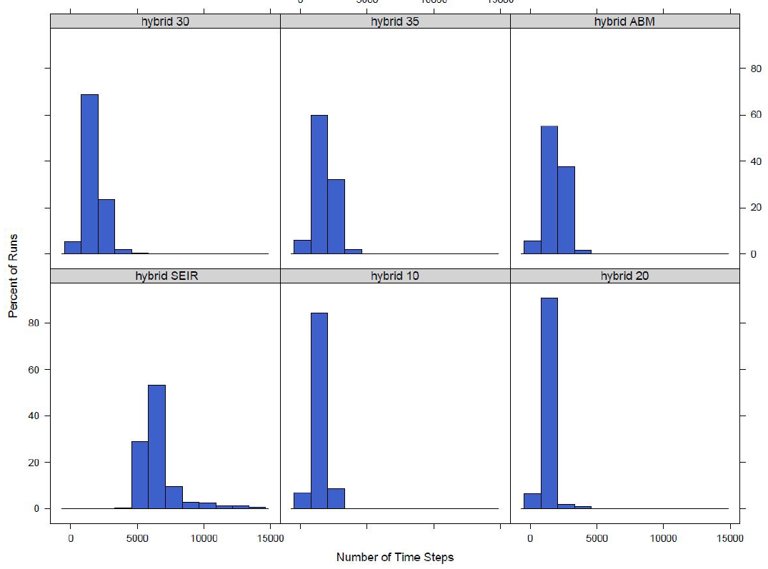
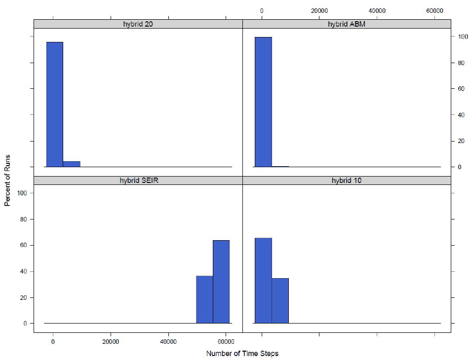
For both the town switch and the small area switch models for the switch values we look at the model switches to an equation-based model in a majority of the runs. This, however, only measures if a model switches over for at least one time step. While it is a good starting point to look at if the disease model is actually switching between agent-based and equation-based, the length of time a model switches for should also be studied. To do this we find the number of time steps the model is using an equation-based disease model. The distributions for the number of time steps the model switches for the small area switch model and the town switch model can be seen in Figures  1 and  2 respectively.

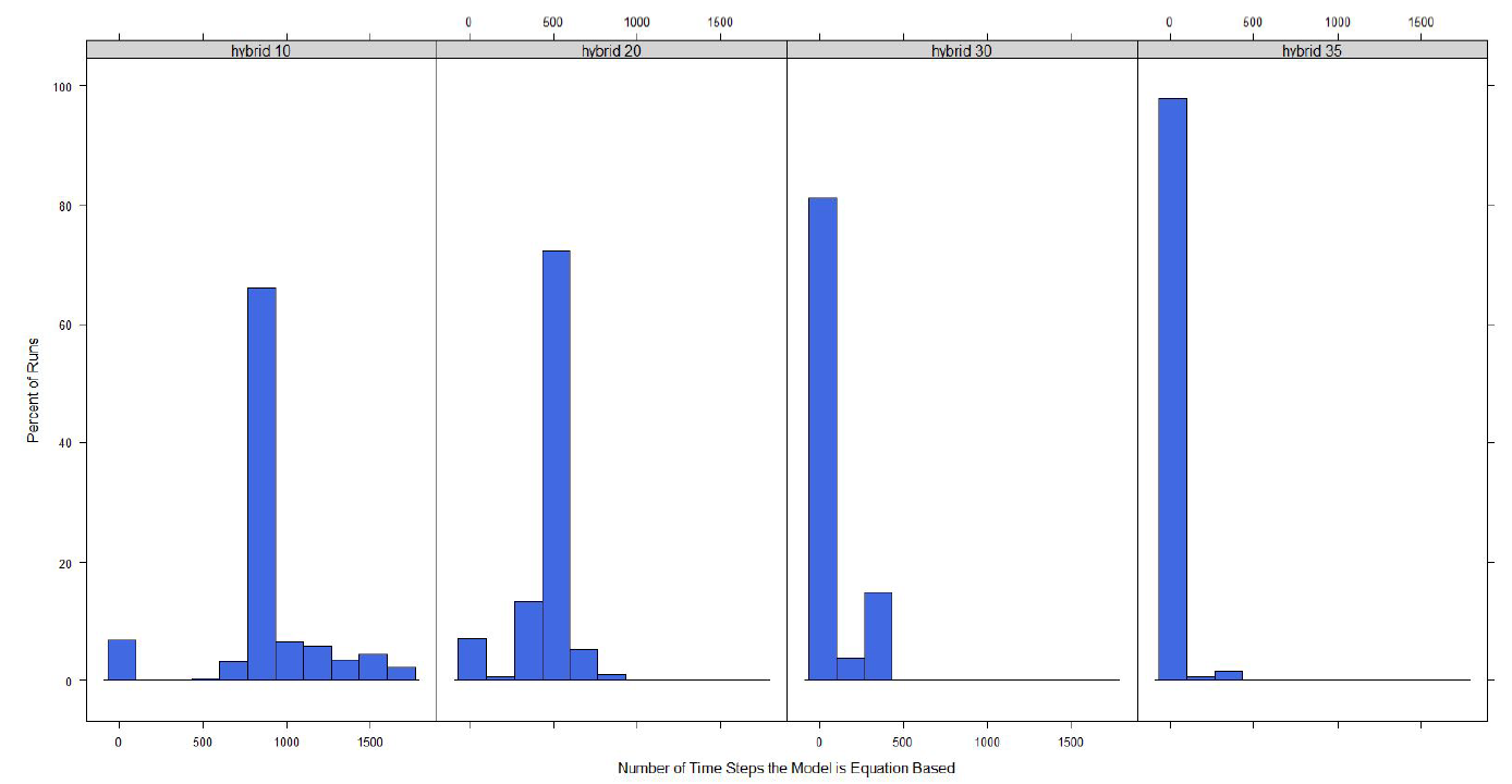
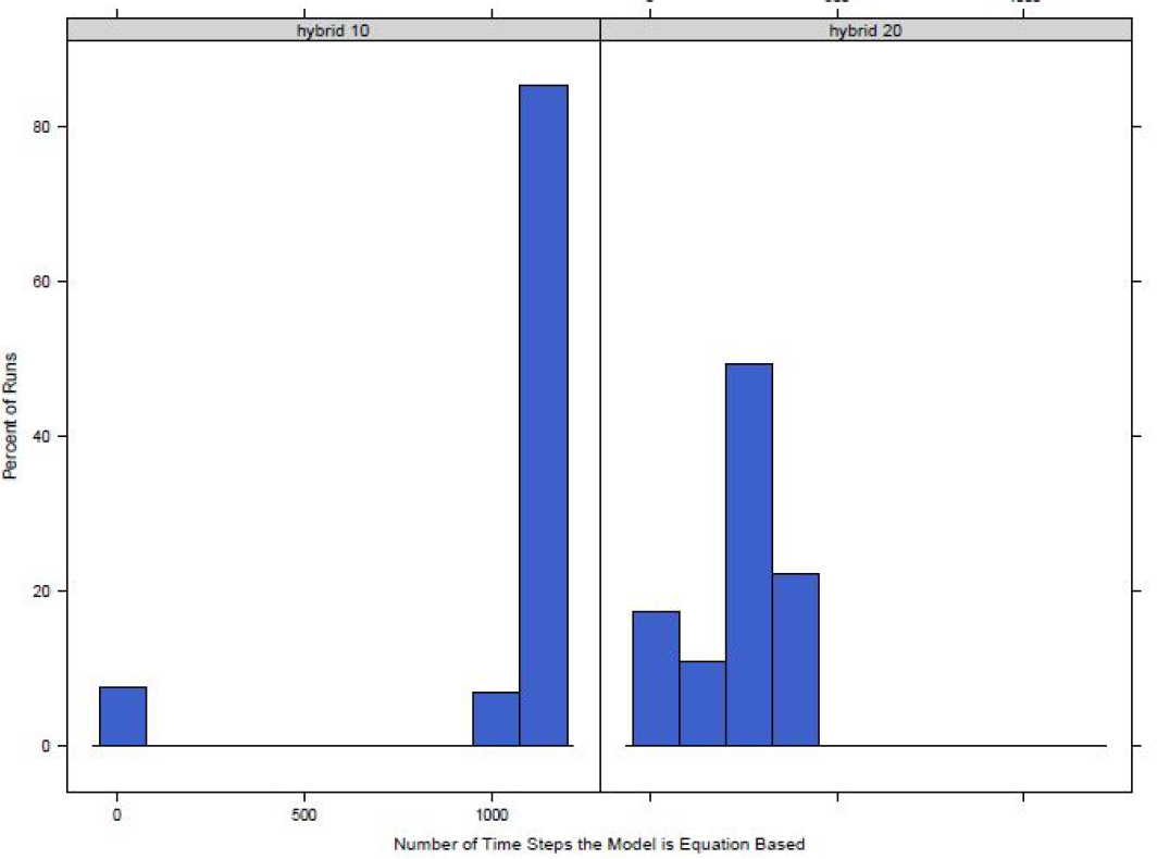
For both models it can be seen that as the switching percentage increases, the number of time steps that use an equation-based model decreases. This is as expected as a higher percentage equates to a larger number of agents required to be exposed or infected before the model switches to equation-based from agent-based and infecting a larger number of agents will take more time steps.

Run Time

Before looking into the results, it is important to determine if using the hybrid will actually result in real savings when running the model. To test for this we find the average number of seconds per time step in each of our versions of the model. Table  2 shows the times for the model with four different switching scenarios: where the disease model is always equation-based, where the model switches to equation-based when 10\(\%\) of agents are infected or exposed, where the model switches to equation-based when 20\(\%\) of agents are infected or exposed, where the disease model is always agent-based. The table also provides a 95\(\%\) confidence interval for the average times. At 30\(\%\) the town model no longer switches from agent-based to equation-based so the values are not shown in the table. At 40\(\%\) the small area switch model switches in less than half of the runs and does not result in any time savings so the results for any switches after 35\(\%\) are not included in the table for either version of the model.

Table 2: Average number of milliseconds for a time step for different versions of the hybrid model switching at the small area level

	time (ms) per time step
Switch	Small Area	Town
Only equation-based Model	1.79	1.90
	\(\textit{(1.59, 1.99)}\)	\(\textit{(1.68, 2.11)}\)
10\(\%\)	2.42	3.55
	\(\textit{(2.14, 2.69)}\)	\(\textit{(3.15, 3.95)}\)
20\(\%\)	4.05	4.61
	\(\textit{(3.59, 4.50)}\)	\(\textit{(4.08, 5.13)}\)
30\(\%\)	5.23	-
	\(\textit{(4.68, 5.87)}\)	-
35\(\%\)	5.77	-
	\(\textit{(5.12, 6.43)}\)	-
Only Agent Based Model	6.77	6.77
	\(\textit{(6.01, 7.54)}\)	\(\textit{(6.01, 7.54)}\)

From the table it can be seen that for the two switching versions, the small area model results in more time saved per time step when compared to the fully agent-based model. In both cases switching over at 10\(\%\) provides greater savings than switching at 20\(\%\). This makes sense as it takes significantly less time per step when the disease model is completely equation-based versus agent-based, therefore, the longer the model stays at agent-based before switching to equation-based the longer the average step length will be. This can be further seen in that the time per step increases in the small area model when the switch is at 30\(\%\) and 35\(\%\). However, the time per step for these two switch points are not significantly different from each other as their values fall with in the others confidence intervals. These results are taken as evidence that the hybrid model is successfully providing time savings in running the agent-based model as compared with the pure agent-based model.

Distribution of Number Infected

After looking at the time saved and the switching behaviours of the model the results are analysed. For each of the different versions of the hybrid model the results are compared to the completely agent-based version of the model. Figure  3 shows the distribution of the number of infected agents across the 300 runs for the small area model at different switch values.

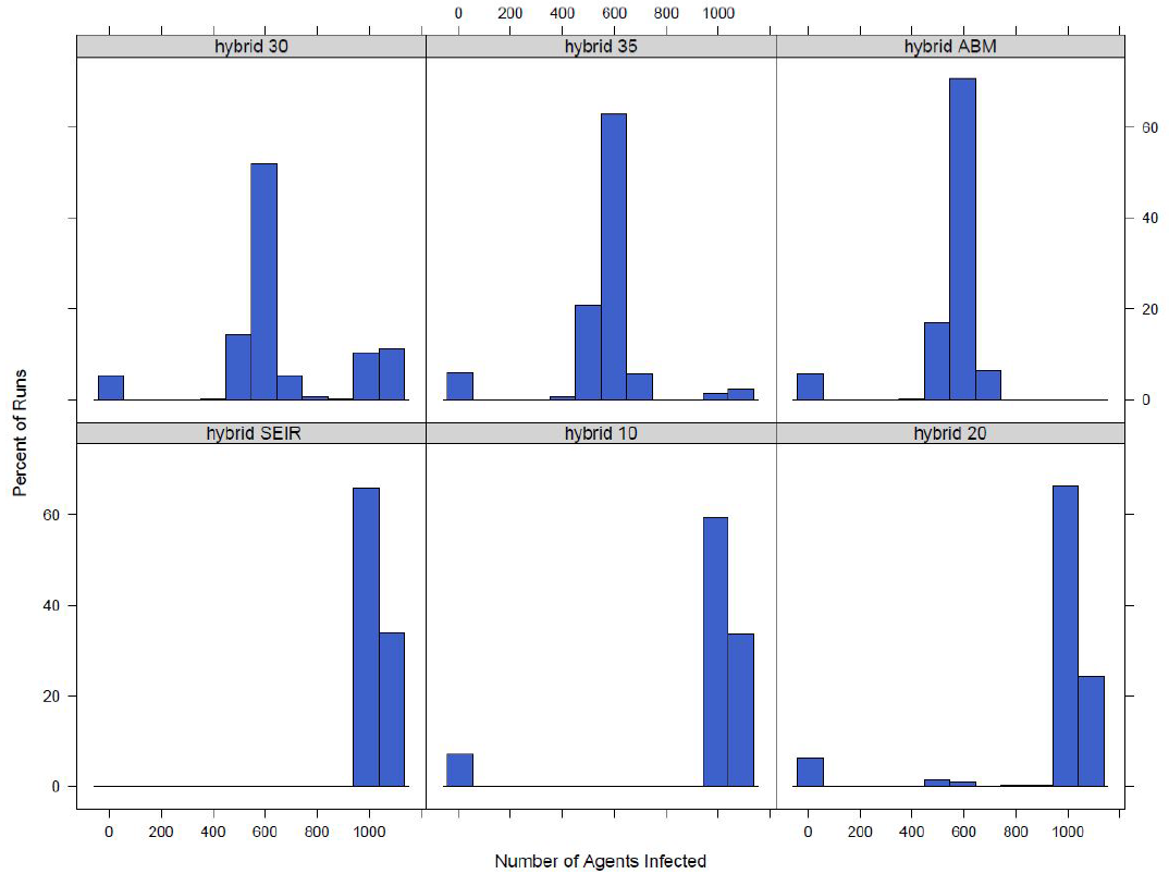
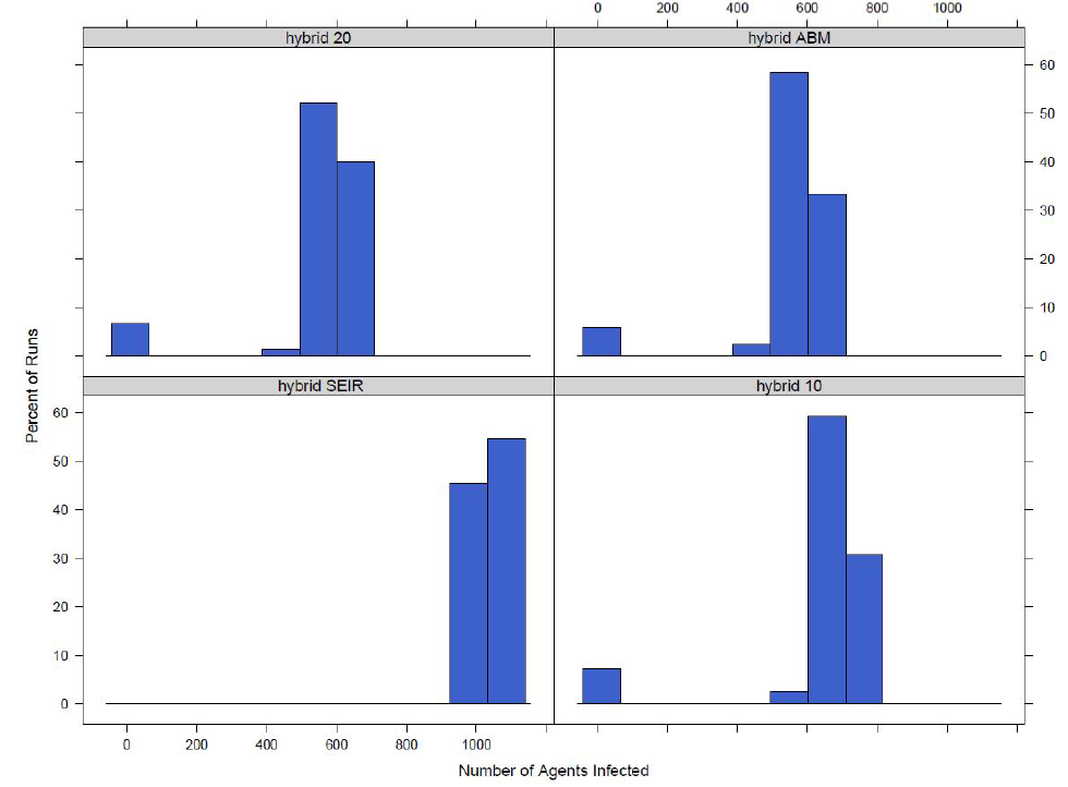
It can be seen in the figure that as the switch gets higher, a higher percent of agents need to be exposed or infected before the model switches to an equation-based model, the distribution moves away from the version of the model where the disease model is strictly equation-based and moves towards the strictly agent-based version. A similar pattern is seen in the town model. The distributions for the model switching at the town level can be seen in Figure  4.

Although it is useful to visualize the change in distribution, it is possible to actually compare the distributions and get a value for the probability that the sample distributions come from the same population. The Wilcoxon rank sum test is a non parametric alternative to a two-sample t-test that does not assume the population distribution is normal. The null hypothesis of the test is that the two populations have the same distribution. A Wilcoxon rank sum test is done for each of our distributions from the switching models compared to the distribution from the completely agent-based model. The p-values for those tests can be found in Table  3.

Table 3: P-values for the Wilcoxon rank sum test comparing the outbreak size distributions for the switching models to the completely agent-based model.

	P-value
Switch	Small Area	Town
10\(\%\)	0.000	0.000
20\(\%\)	0.000	0.015
30\(\%\)	5.9e\(^{-6}\)	-
35\(\%\)	0.5791	-

The values show that as the switch is larger, the distribution gets closer to the agent-based model. This can easily be explained, the larger the switch the longer the model remains agent-based so the more similar the two distributions will be. Our aim was to find a range of switch points that still result in the model switching between an agent-based and equation-based disease model but results in a distribution that is similar to the complete agent-based model. From the table we can see that a switch of 35\(\%\) at the small area level results in a distribution that is not significantly different from the purely agent-based model and that a switch of 20\(\%\) at the town level results in a distribution that is not significantly different from the agent-based model distribution at a 1\(\%\) significance level.

Length of outbreak

Finally the total time it takes for an outbreak to finish is investigated. An outbreak is considered finished if there are no agents exposed or infected within the model. The outbreak length is studied because it is another important characteristic of model output. If the hybrid model has a similar outbreak size but a different outbreak length than its not possible to say that the outbreaks are similar. The distributions of the number of time steps it takes for the outbreak to finish for the small area switching model and the town switching model can be seen in Figure  5 and Figure  6 respectively.

Similar to the total outbreak size distributions, the outbreak length distributions converge to the completely agent-based model distribution. Again the Wilcoxon rank sum test is used to compare the time distributions. The values can be found in Table  4. From the table it can be seen that as switch increases the distribution gets closer to that of the agent-based model. For the switch at the small area level we can see that when the switch is 35\(\%\) the distributions are not significantly different at the 10\(\%\) significance level and for the switch at the town level when the switch is at 20\(\%\) the distributions are not significantly different at the 5\(\%\) level.

Table 4: P-values for the Wilcoxon rank sum test comparing the outbreak time distributions for the switching models to the completely agent-based model.

	P-value
Switch	Small Area	Town
10\(\%\)	0.000	0.000
20\(\%\)	0.000	0.0707
30\(\%\)	1.6e\(^{-7}\)	-
35\(\%\)	0.1036	-

Discussion

Based on the above results we can see that the hybrid model is able to switch between agent-based and equation-based for a majority of runs when the switch is 35\(\%\) or below and switching at the small area level and 20\(\%\) or below and switching at the town level. In addition, at all values of the switch considered we see that there are significant time savings when running the hybrid model over the purely agent-based model. The experiments to analyse the fidelity of the hybrid model show that at lower switch values, the hybrid model distributions for both the total number of agents infected and the length of the outbreak are significantly different from the agent-based model distributions. However, at a switch of 35\(\%\) for the small area switch and 20\(\%\) for the town switch statistical tests show that there is not a significant difference between the hybrid and agent-based distributions. Although both the small area and town level models result in time savings and produce significant results, the time savings are greater at the town level as the town level switch converges faster to the agent-based model results. A hybrid model switching at the small area level with a threshold switch of 35\(\%\) is statistically similar to a fully agent-based model and has a time savings of an average of one millisecond per time step while a hybrid model switching at the town level with a threshold of 20\(\%\) is also statistically similar to a fully agent-based model but has a time savings of an average of 2.16 milliseconds per time step. Because of this we feel that switching at a town level over a small area level provides a greater advantage.

County Hybrid Model

The hybrid model for a single town is a start in an analysis to show that a hybrid model can succeed in both saving time and computing power when running a large agent-based model. The results show that not only does a hybrid model save computing time compared to a fully agent-based model but the results also start to converge to the results for the agent-based model as the switch point changes. However, even though in most cases the models appear to be converging the results are still shown to be from different distributions based on the Wilcoxon rank sum test and any larger switch values will not save time or result in the model actually switching. One factor causing this could be that the model is run on a small town. With only about 1,000 agents in the entire model switching can only happen on a small scale. In addition, at such a small scale the fully agent-based model does not take too much time to run leading to advantages in time saved for the hybrid model being negligible in many cases. To show the true advantage of a hybrid model it will be necessary to start with a model that is much larger where saving time can be done on a larger scale. To do this a county model is used. The county model is an adapted version of the Hunter et al. (2020) model.

Model components

The following sections give a brief overview of the county model describing the four main components of an agent-based model outlined in Hunter et al. (2017). The process to create and setup the environment and the society component do not change from the model in Section 4. However, changes are made to the transportation component in order to scale up the model¹ and switching between the agent-based disease component and the equation-based disease component changes. The changes to the transportation component and the switching behaviour are described in the following sections.

Transportation component

Parts of the transportation model differ between the town model and the county model. Agents will still move in one step from their location to their desired destination and some movements are predetermined by the model with the agents moving between home and school or home and work at certain times. However, commuting patterns within the model are determined using CSO Place of Work, School or College - Census of Anonymity Records (POWSCAR) data (CSO 2017). This dataset provides information on the commuting patterns of people in Ireland.

The random movements throughout the community when agents are not at home, school or work are also changed in the transportation model. While we think random movements is an acceptable modelling simplification when modelling a small town with a closed population, when modelling a county it is no longer acceptable to assume random movements throughout the county: it is much more likely that an agent will remain in their own town or go to a town next door in the next hour than that they will be on the other side of the county. To account for this we use a gravity type model for transportation. A gravity model determines those interactions between two location pairs based on the characteristics of a location and the distance between locations (Comtois & Slack 2006). The probability of an agent moving to another small area is proportional to the population density of the small area, an area that has a lot of other agents is more attractive, and inversely proportional to the distance to the small area from the agent’s current location, areas that are farther away are less attractive. Admittedly the attractiveness of a location is not always correlated with population density (for example, special attractions, such as monuments, may be located away from population centres), however we believe that using a population density based gravity model to drive movement at the a county level provides a reasonable trade-off between model simplicity and realism at this geographic scale, and so provides a more accurate simplification of movement within a larger area than that in the original town model.

Disease component

Both the agent-based and equation-based disease components of the model are the same as that of the town model. Switching is also similar, however, the county model switches at either the town level or the whole county level. The model being used in a given time step by the town is determined by the number of agents infected in either the town or the whole county. Similar to in the town model, it is important to note that if the switch is 0\(\%\), the model will switch from agent-based to equation-based when 0\(\%\) of agents are exposed or infected, this means the disease component of the model will always by equation-based and if the switch is at 100\(\%\) the model will always be completely agent-based. However, when the disease model switches at the county level, there is one set of difference equations for the whole county, the model is essentially completely equation-based. Even though agents are allowed to move, because agents are infected at the county level their location does not have an influence on if the agent will be infected or not. The model with a switch of 0\(\%\) has no stochasticity in it and the only thing that would have an impact on the results is the initial conditions: if the model starts with more or less agents, more than one agent infected, or there are a number of agents who are already immune.

Experiments and results

To test the county hybrid model we run similar experiments to those presented in Section 4 to look at the switching behaviour of the model, the time savings and the fidelity of the results when compared to the fully agent-based model. We do one additional fidelity test for the hybrid model to compare how the outbreak spreads through the network of towns in the county.

For both the town switch and the county switch we look at the switch values of 0\(\%\), 5\(\%\) and 10\(\%\) and we also look at switches at 20\(\%\) and 30\(\%\) at the town level. Similar to the town model, the smaller geographic area, town, continues to switch between the agent-based and equation-based disease component at a higher threshold compared to the larger geographic area, county, because the actual number of agents needed to be exposed and infected at the same time is smaller for the town than the county with the same switching threshold. For each switch value except for 0\(\%\) we run the model 300 times. As mentioned in the previous section, there is no stochasticity in the model with a switch of 0\(\%\) at the county level, so the model only needs to be run once to get the results.

Number of runs that switch

In order to make sure the model is utilizing the hybrid architecture we look at a number of measures: the number of time steps that the model has switched to hybrid and the maximum number of towns that have switched to hybrid during the model.

Table 5 shows the percent of runs for each of the switch values that results in the model switching to an equation-based disease component for at least one time step.

Table 5: Percent of runs that lead to the model switching from agent-based to equation-based

	Percent of Runs that Switch
Switch	Town	County
5\(\%\)	76.3	89.7
	\(\textit{(71.5, 81.1)}\)	\(\textit{(86.2,93.1)}\)
10\(\%\)	73.3	88.0
	\(\textit{(68.3, 78.3)}\)	\(\textit{(84.3, 91.7)}\)
20\(\%\)	75.3	-
	\(\textit{(70.5, 80.2)}\)	-
30\(\%\)	69.3	-
	\(\textit{(64.1, 74.6)}\)	-

The table shows that for all versions of the switch the model becomes equation-based for a large portion of runs. It can also be seen from the model that it is more likely for a switch to occur if the model is switching at the county level versus the town level. However, as noted in the previous section if the switch value is 20\(\%\) the model switching at the county level will not switch to equation-based.

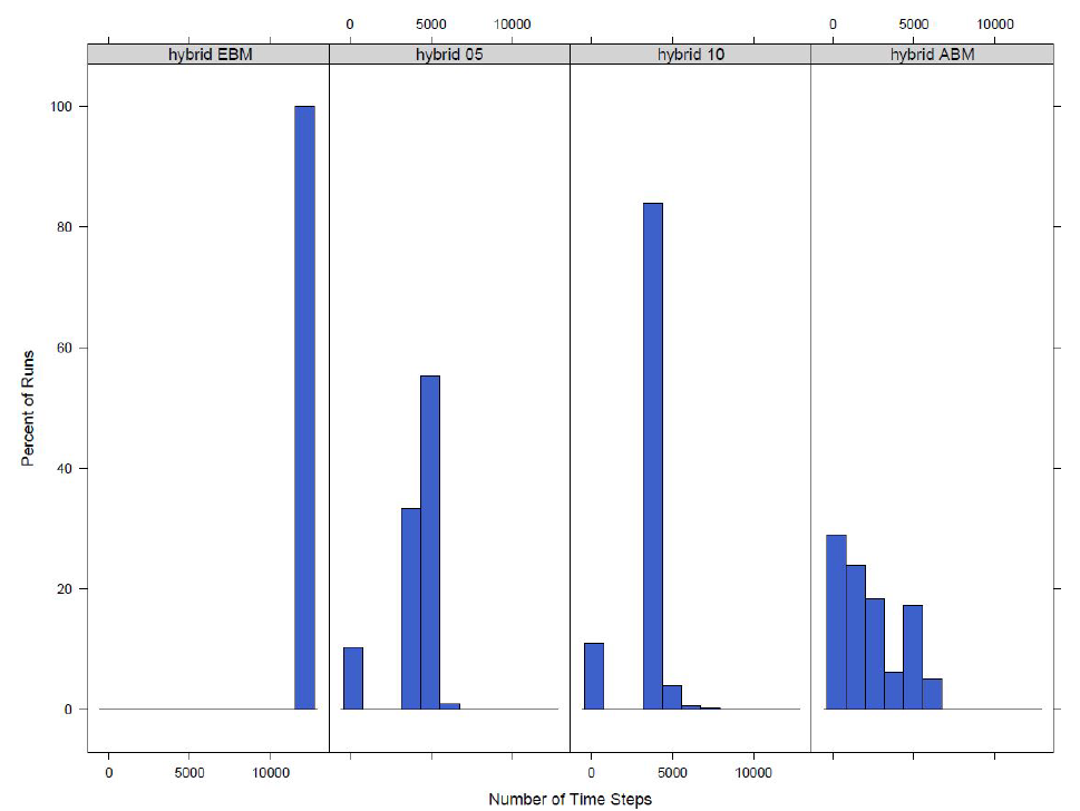
A run is counted in the percentages in Table  5 if it has switched to equation-based for at least one time step, but models switching for only one or two time steps are not taking full advantage of the hybrid architecture of the model. Thus we look at the distributions of the number of time steps that have switched from agent-based to equation-based. Figure  7 shows the distribution when switching at the town level and Figure  8 shows the distribution when switching at the county level.

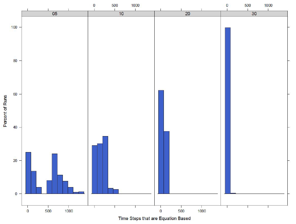
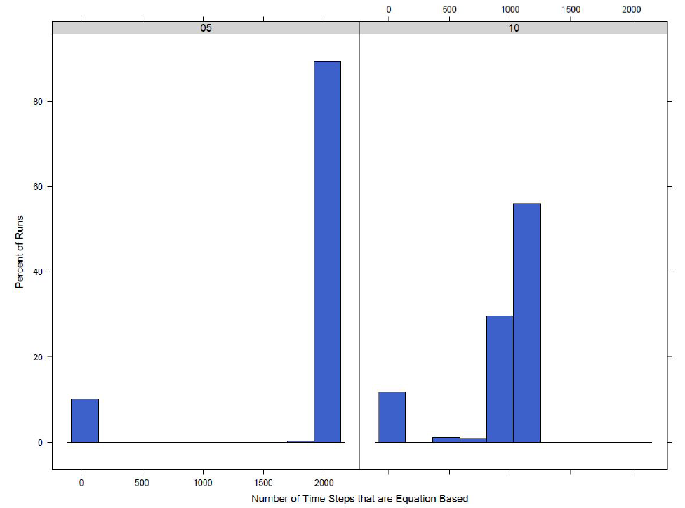
Looking at the distributions of the count of time steps where the model has switched to an equation-based disease model it can be seen that when the switch value is lower, the number of time steps where at least one town has switched to equation-based increases. This is as expected and makes sense as the model should reach the point where 5\(\%\) of agents are infected or exposed before 30\(\%\) of agents are infected or exposed and thus will remain equation-based for longer.

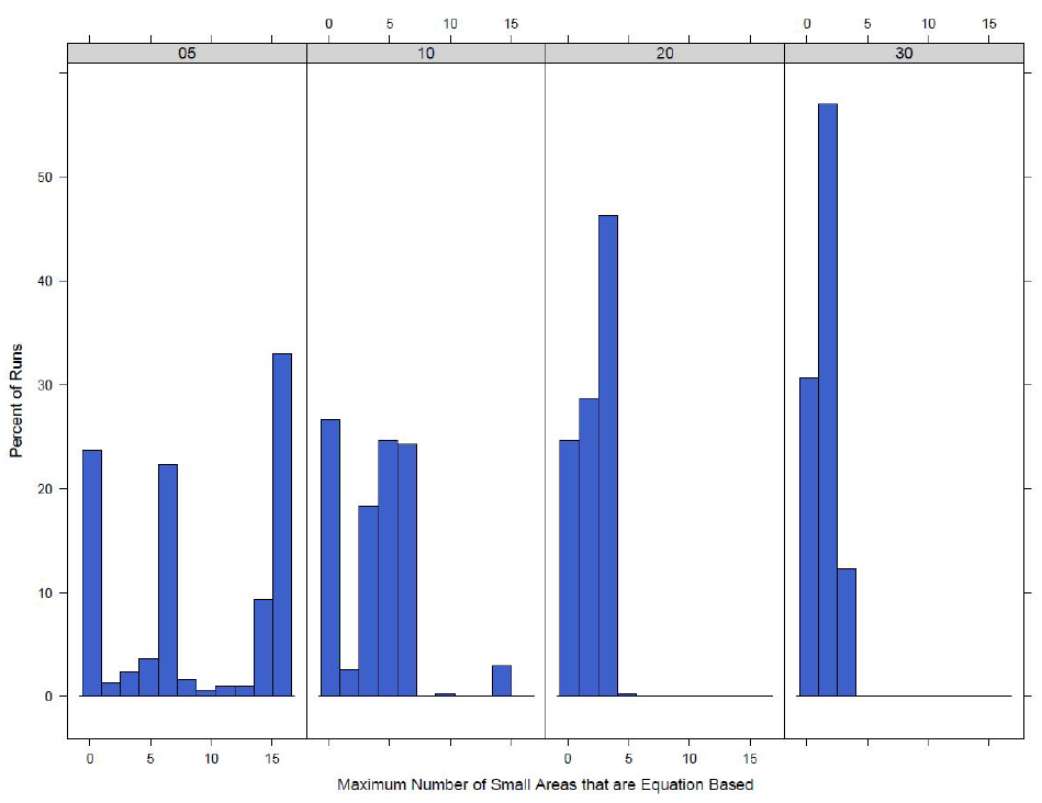
The maximum number of small areas that have had their town switch to an equation-based model can be found in Figure  9. This is only done for the town switch model because when the model switches at the county level all towns switch together at the same time. As expected the model with a lower switch value has a higher maximum number of small areas that have switched to equation-based. The town switch model does not result in a larger portion of the model switching at any one time. With a switch of 5\(\%\) the maximum number of small areas switched is 16 out of a total of 173 small areas in the county. This number reduces even more as the switch increases to 30\(\%\) with only a maximum of 4 small areas in the equation-based model at any given time step.

Run time

Similar to the run time experiment in Section 4 we look at the run time of the model to determine if the hybrid model produces savings over the fully agent-based model. Table  6 shows the results for the average time in seconds for each time step in the model.

Table 6: Average number of seconds for a time step for different versions of the hybrid model

	time (s) per step
Switch	Town	County
equation-based Model	0.82	0.64
	\(\textit{(0.66, 0.98)}\)	\(\textit{(0.52, 0.77)}\)
5\(\%\)	1.00	0.87
	\(\textit{(0.80, 1.20)}\)	\(\textit{(0.70, 1.04)}\)
10\(\%\)	1.04	1.21
	\(\textit{(0.84, 1.25)}\)	\(\textit{(0.97, 1.44)}\)
20\(\%\)	1.28	-
	\(\textit{(1.03, 1.53)}\)	-
30\(\%\)	1.36	-
	\(\textit{(1.09, 1.63)}\)	-
Only Agent Based Model	1.40	1.40
	\(\textit{(1.12, 1.67)}\)	\(\textit{(1.12, 1.67)}\)

From the table it can be seen that there is almost half a second time savings per step going from a full agent-based model to a model where the disease component switches to equation-based when 5\(\%\) of the agents are infected or exposed. Additionally we can see that when the model switches when there are 20\(\%\) or 30\(\%\) of agents infected or exposed, there are not significant time savings when compared to the completely agent-based model.

A similar time saving of over a half second per time step can be seen in the model that switches at the county level going from the agent-based model to the hybrid model that switches at 5\(\%\) infected and exposed. However, even though the average number of seconds per time step is 0.2 seconds less than the agent-based model when the switch is 10\(\%\), the average value falls within the confidence interval of the agent-based model and vice versa showing no significant difference.

Distribution of Number Infected

Determining the time savings and the switching behaviour of the the model allows us to determine if the hybrid architecture is both working by saving time and resulting in the model switching between agent-based and equation-based for an extended period of time. Once it is determined that the model is working, it is necessary to look at how the results of the hybrid model compare to the complete agent-based model. The distribution of the total number of infected agents across the runs for the different switching points can be found in Figure  10.

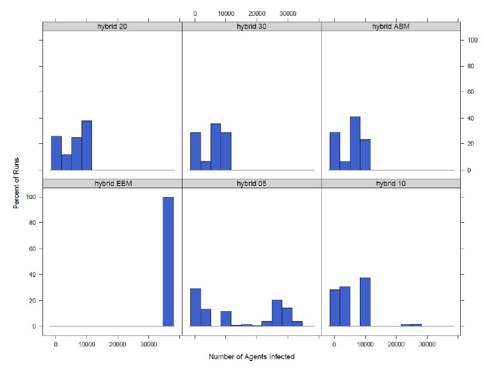
From the figure it can be seen that the distributions for switching at 20 or 30\(\%\) infected or exposed are similar to the fully agent-based model. Switching at 10\(\%\) infected or exposed results in a similar distribution, however, there appear to be some more obvious differences, such as a small cluster of outliers to the right of the distribution representing a number of runs with a much higher number of total infected agents. It can also be noted that comparing the 10\(\%\) switching model to the fully agent-based model that there is a higher number of runs with a smaller number of infectious agents when the model switches. The distribution for the 5\(\%\) switching model looks distinctly different from the rest of the models. The 5\(\%\) switching model results in a distribution with a much larger number of agents infected then any of the other models. All of the switching hybrid models are different from the model where the disease component is fully equation-based, however it can be seen how the model results move farther from the equation-based disease component model as the switch increases. The differences in the equation-based model, 5\(\%\), 10\(\%\), and full agent-based model help to show why agent-based models are important. When homogeneous mixing is present in the model, the equation-based disease model, a higher number of agents can become infected. This is because all agents have equal probabilities of coming into contact with each other if they are in the same town. However, when heterogeneous mixing is used in the model (the agent-based disease model) there are fewer infected agents because agents are less likely to infect someone outside of their social networks.

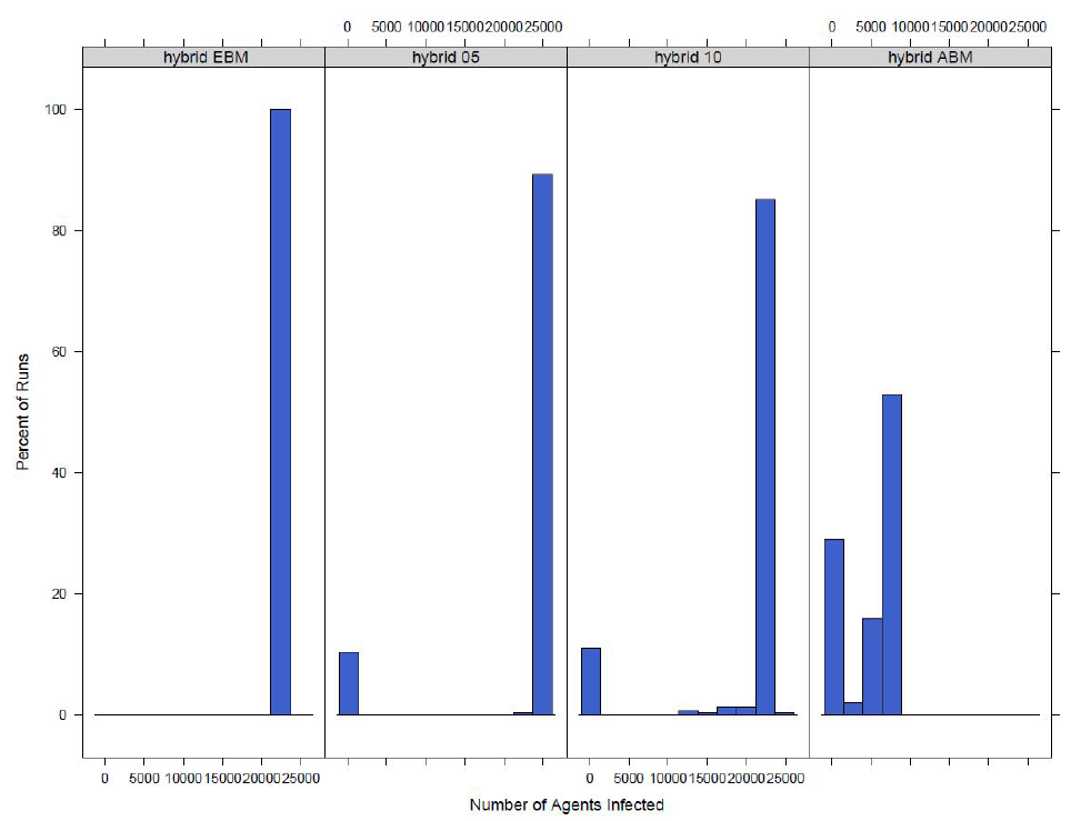
A similar analysis is done when the switch is at the county level. The distribution of the total number of infected agents can be found in Figure  11. From the figure it can seen that the models that switch from an agent-based to an equation-based disease component appear more similar to the model with an equation-based disease component then an agent-based disease component. They do, however, appear to be slowly converging towards the agent-based results.

To further compare the similarities of the distributions, the Wilcoxon signed-rank test is run comparing the hybrid models to the completely agent-based model. The tests are used to determine if two sample distributions come from the same population. Table  7 shows the p-values for the tests comparing each hybrid models to the fully agent-based model.

Table 7: P-values for the Wilcoxon rank sum test comparing the outbreak size distributions for the switching models to the completely agent-based model.

	P-value
Switch	Town	County
5\(\%\)	4.861e\(^{-12}\)	2.2e\(^{-16}\)
10\(\%\)	0.1625	2.2e\(^{-16}\)
20\(\%\)	0.2942	-
30\(\%\)	0.9566	-

The p-values further show what was seen Figure 10. For the model that switches at the county level, the p-values are close to 0 meaning that the null hypothesis of the distributions coming from the same population should be rejected. Thus switching at the county level does not result in distributions of infected agents that are similar to the agent-based model. When the switch is at the town level, the distribution with a 5\(\%\) switch value has a p-value very close to 0 so the null should be rejected as well. However, the distributions for 10\(\%\), 20\(\%\), and 30\(\%\) are not significantly different from the agent-based model.

Length of outbreak

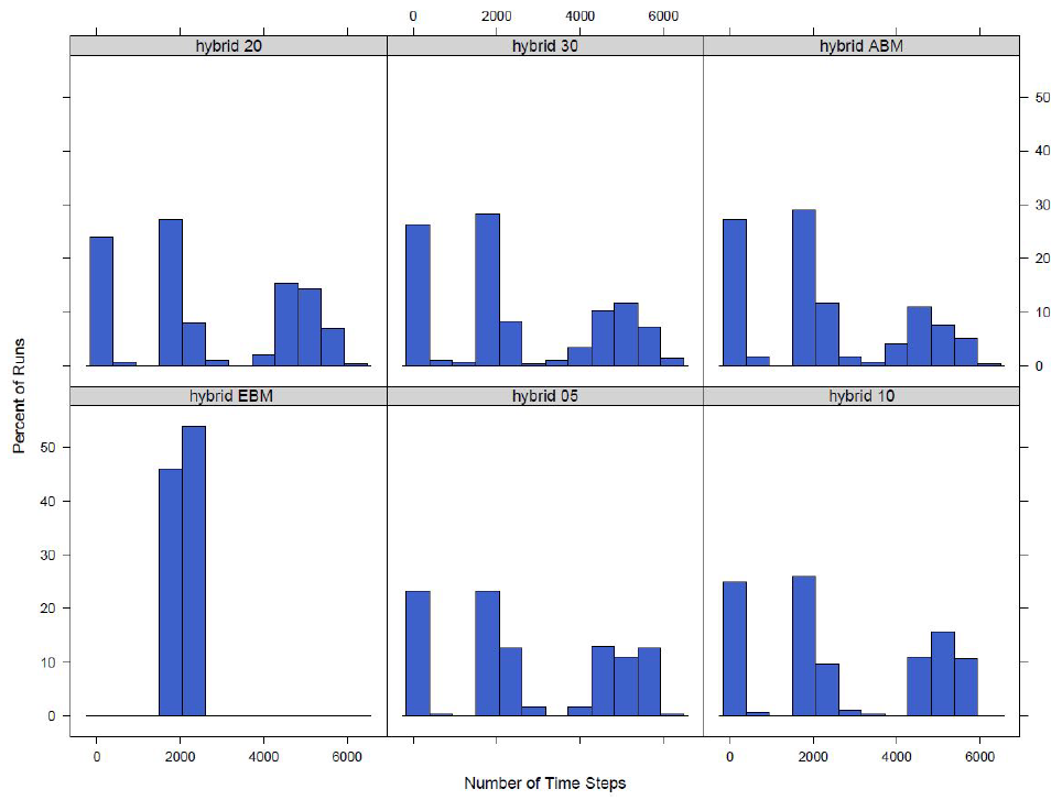
To compare our outbreaks we also look at the time it takes for the outbreak to finish. An outbreak is complete when there are no longer any exposed or infected agents in the model. If the run times of the models are drastically different it will be hard to compare the results as the outbreak length is a key descriptive feature of an outbreak. To compare the lengths of outbreaks across models the distributions of the the number of time steps taken for the model to finish is looked at for both versions of the model and each switch value. The distribution for the model that switches at the town level can be seen in Figure  12.

A similar analysis is done for the model that switches at the county level. The distribution of the number of time steps that it takes for the model to finish for each of the four different versions of the model is found in Figure  13. Similar to the distribution of number of agents infected it can be seen that the number of time steps it takes for the model with a completely equation-based disease component is distinctly different then the fully hybrid model. The two versions of the model that switch between the agent-based and equation-based disease components have a distribution of time steps in between the equation and agent-based versions.

The p-values for the Wilcoxon tests to compare the hybrid models to the agent-based model can be seen in Table  8, the p-values for the models that switch at 5\(\%\), 10\(\%\) and 20\(\%\) are all small meaning there is only a small probability that the distributions are from the same population. The distributions for the number infected that are from the model that switch at the county level show clear differences between the complete agent-based and the hybrid models. This can be further seen in the p-values from the Wilcoxon tests that are very near zero.

Table 8: P-values for the Wilcoxon rank sum test comparing the outbreak length distributions for the switching models to the completely agent-based model.

	P-value
Switch	Town	County
5\(\%\)	0.0021	2.2e\(^{-16}\)
10\(\%\)	0.0143	2.2e\(^{-16}\)
20\(\%\)	0.0160	-
30\(\%\)	0.2283	-

Spread of the outbreak

Another aspect of the outbreak that can be considered is what towns the outbreak spreads to. As the model is run in a scenario with a highly infectious disease and the population has no previous immunity, there is a large number of infected agents in the model.

Table  9 shows the percent of runs that lead to an outbreak in the switch model for twelve different towns in Leitrim County along with the population of the town and a weighted degree centrality. The degree centrality is a measure of the number of agents that commute in and out of the town. Six of the towns are larger towns that are made up of multiple small areas, Ballinamore, Dromahair, Leitrim, Lurganboy, Manorhamilton, and Mohill. The other six towns are smaller towns that are only made up of one small area, Aghacashel, Corrala, Glenfarn, Newtowngore, Munakill and Rinn. The results are given for each version of the model based on the switch and the fully agent-based model. The version of the model with the fully equation-based disease component is not included as the model results in nearly all the agents becoming infected every run, thus every town would have an outbreak in it each run. From the results it can be seen that for the larger towns, the majority of the runs result in outbreaks and for the completely agent-based model all of the larger towns have 71\(\%\) of runs that lead to an outbreak. This is the same percent as the percent of runs that leads to an outbreak in the overall model, with 71\(\%\) of runs having at least two agents in the county infected. This is likely because the model is run without immunity to be able to fully test out the hybrid model and therefore for a larger town that is likely more central with more agents commuting in and out when there is an outbreak in the county where no agents are immune it will spread to the larger towns. As the smaller towns have fewer agents they are not as likely to have the outbreak spread to them.

Table 9: Percent of runs that the outbreak spreads to the given town

Town	Centrality	Population	5\(\%\)	10\(\%\)	20\(\%\)	30\(\%\)	Agent-Based
Aghacashel	0.05	73	33.3	16.3	15.7	12.3	10.0
			\(\textit{(28.0, 38.7)}\)	\(\textit{(12.2, 20.5)}\)	\(\textit{(11.6, 19.8)}\)	\(\textit{(8.6,16.0)}\)	\(\textit{(6.6, 13.4)}\)
Ballinamore	0.44	1096	76.3	74.0	75.3	72.0	71.0
			\(\textit{(71.5, 81.1)}\)	\(\textit{(6.09.0, 79.0)}\)	\(\textit{(70.5, 80.2)}\)	\(\textit{(66.9, 77.1)}\)	\(\textit{(65.9, 76.1)}\)
Corrala	0.14	248	64.0	56.3	56.3	58	51.3
			\(\textit{(56.3, 69.4)}\)	\(\textit{(50.7, 61.9)}\)	\(\textit{(50.7, 61.9)}\)	\(\textit{(52.4, 63.6)}\)	\(\textit{(45.7, 57.0)}\)
Dromahair	0.15	1506	76.3	74.3	75.3	72.3	71.0
			\(\textit{(71.4, 81.1)}\)	\(\textit{(69.4,79.3)}\)	\(\textit{(70.5, 80.2)}\)	\(\textit{(67.3, 77.4)}\)	\(\textit{(65.9, 76.1)}\)
Glenfarn	0.03	147	52.7	35.0	32.3	28.7	27.7
			\(\textit{(47.0, 58.3)}\)	\(\textit{(29.6, 40.4)}\)	\(\textit{(27.0, 37.6)}\)	\(\textit{(23.4, 33.8)}\)	\(\textit{(22.6, 32.7)}\)
Leitrim	0.21	1123	76.3	74.3	75.3	72	71.0
			\(\textit{(71.5, 81.1)}\)	\(\textit{(69.4, 79.3)}\)	\(\textit{(70.5, 80.2)}\)	\(\textit{(66.9, 77.1)}\)	\(\textit{(65.9,76.1)}\)
Lurganboy	0.00	388	76.3	74.3	75.3	72	71.0
			\(\textit{(71.5, 81.1)}\)	\(\textit{(69.4, 79.3)}\)	\(\textit{(70.5, 80.2)}\)	\(\textit{(66.9, 77.1)}\)	\(\textit{(65.9, 76.1)}\)
Manorhamilton	1.00	1782	76.3	74.3	75.3	72.3	71.0
			\(\textit{(71.5, 81.1)}\)	\(\textit{(69.4, 79.3)}\)	\(\textit{(70.5, 80.2)}\)	\(\textit{(67.3, 77.4)}\)	\(\textit{(65.9, 76.1)}\)
Mohill	0.86	1378	76.3	74.0	75.3	72.0	71.0
			\(\textit{(71.5, 81.1)}\)	\(\textit{(69.0, 79.0)}\)	\(\textit{(70.4, 80.2)}\)	\(\textit{(66.9, 77.1)}\)	\(\textit{(65.9, 76.1)}\)
Munakill	0.12	196	62.3	55.0	57.3	56.0	45.7
			\(\textit{(56.9, 67.8)}\)	\(\textit{(49.4, 60.6)}\)	\(\textit{(51.7, 62.9)}\)	\(\textit{(50.4, 61.6)}\)	\(\textit{(40.0, 51.3)}\)
Newtowngore	0.14	230	62.0	45.3	42.7	38.3	39.3
			\(\textit{(56.5, 67.5)}\)	\(\textit{(39.7, 51.0)}\)	\(\textit{(37.1, 48.3)}\)	\(\textit{(32.8, 43.8)}\)	\(\textit{(33.8, 44.9)}\)
Rinn	0.36	293	66.7	61.3	68.7	64.7	58.7
			\(\textit{(61.3, 72.0)}\)	\(\textit{(55.8, 66.8)}\)	\(\textit{( 63.4, 73.9)}\)	\(\textit{(59.3, 70.1)}\)	\(\textit{(53.1, 65.2)}\)

It can also be seen from Table 9 that as the model gets closer to the fully agent-based model, the switch increases in size, the results are more similar to the fully agent-based model, further showing how the hybrid model converges to the hybrid as the switch increases. The percent of runs that lead to an outbreak is also calculated for the model with the county level switch. However, when the model that switches at the county level switches to an equation-based disease component from an agent-based disease component the location of an agent does not have an influence on if they become infected and there is homogeneous mixing for all agents in the model. Thus the percent of runs that lead to an outbreak for the model switching at the county level when 5\(\%\) of agents are infected or exposed and when 10\(\%\) of the agents are infected or exposed is equal to the number of runs that spread outside of a single town in model. This shows a clear difference between the model that switches at the town level and the model that switches at the county level. The town switch still allows for agents movement patterns, such as their commutes to influence the spread of the outbreak. Even though the larger more central towns in the model have similar percent of runs that lead to an outbreak, the smaller less central towns have more variable results. This is not the case in the model that switches at the county level where the outbreak is equally likely to spread to all towns regardless of the size and centrality.

Conclusion

Hybrid models allow us to utilize the advantages of two different modelling techniques. The paper shows that it is possible to create a hybrid model for infectious disease epidemiology where the disease component switches between agent-based and equation-based determined by the number of agents infected. We looked at a number of levels for switching, both at the actual value of the switch (5\(\%\), 10\(\%\) etc.) and at the size of the area where the switch occurs (small area, town or county). For each version of the hybrid model we compared the results to the fully agent-based model and found that a number of factors influence the results of the hybrid model. The value of the switch, if the model turns to equation-based at 5\(\%\) or 30\(\%\) infected is important as it determines the initial conditions. The higher the switch the less likely it will be that the model switches and switches for an extended period of time. The higher switch values do not result in as much savings of time and computing power as the lower switch values. In addition, these models were run on a scenario where the entire population was susceptible to the disease. While this may be the case for new and emerging diseases, for a disease such as or influenza a portion of the population will be already immune to the disease. This will create even less opportunity for switching at a higher percent of agents infected or exposed.

Another factor influencing the results of the model is the area over which the switch occurs. From our test we have looked at a number of levels from small area to town to county. The results of our model show that the smaller the area of the switch the less time saved, this is because at the lower levels the equation-based and agent-based disease components will be running simultaneously based on the number infected at each town so more of the model will be agent-based even when the model has switched. However, at the county level the entire model will be equation-based at once so there is more time savings. In addition, the size of the area that is switched has an impact on how similar the results will get to the agent-based model and the largest switch value that can best used. The smaller the area that is switching the larger the switch can be. For example, when we switched at the small area level the model still switches at values up to 35\(\%\) but the county model only switches to about 10\(\%\) . We can also see that when the switch is at the town level the hybrid model converges to the agent-based model faster than if the the switch is at the small area level or the county level.

Our analysis leads us to the conclusion that at both levels of the model, town and county, the switch for our hybrid model is best done at the town level. We think that the town level switch provides sufficient time savings compared to a fully agent-based model while still being able to produce results that are similar to the fully agent-based model. Not only do we capture a similar distribution of the number of infected agents but the county model is also able to capture a similar spread of the outbreak through the county. Further based on the analysis a switch value between 5\(\%\) and 20\(\%\) is likely going to produce the best results. A switch closer to 20\(\%\) will better match the agent-based model but a switch closer to 5\(\%\) will result in greater time savings and more time steps with an equation-based disease component.

Generally, in creating a hybrid model there is a large amount of flexibility. We chose to use a switch between agent-based and equation-base models and to only switch the disease component. Others might choose different structures and thus the aggregation and switch that we suggest here would not be applicable to their models. However, we feel that the method of testing, by comparing the hybrid model results at different thresholds of switching and different levels of aggregation to the fully agent-based model is a valid method for testing a hybrid model that involves a switching behaviour.

Further work can be done to improve the model, to make the model more realistic it should be tested where there is already some level of immunity in the population. This should require lower levels of switching and may produce different comparative results than what we have presented here. The difference equation model that we use for the equation-based portion of the model is simple. There are ways to create a more realistic equation-based model, for example, adding additional equations for age groups. However, every additional equation makes the model more complicated and will cause additional run time. The idea of creating a hybrid agent-based and equation-based model is to simplify the model and save time and computing. Therefore, any work to further complicate the equation-based model should keep that in mind. Additionally, as the model was created for the spread of measles, schools are considered the main sources of transmission. Going forward additional work should be done to focus on other areas of transmission that might be more relevant to other infectious diseases. For example, including public transportation, shopping centers, gyms and large events such as concerts. Further the simplified gravity model can be made more realistic by adding in special attractions such as monuments and national parks that might draw agents to a particular location.

References

ALLEN, L. J. S. (1994). Some discrete-time SI, SIR, and SIS epidemic models. Mathematical Biosciences, 124(1), 83-105. [doi:10.1016/0025-5564(94)90025-6]

BARRETT, C. L., Bisset, K. R., Eubank, S. G., Feng, X., & Marathe, M. V. (2008). EpiSimdemics: An efficient algorithm for simulating the spread of infectious disease over large realistic social networks. International Conference for High Performance Computing, Networking, Storage and Analysis. [doi:10.1109/sc.2008.5214892]

BINDER, B. J., Ross, J. V., & Simpson, M. J. (2012). A hybrid model for studying spatial aspects of infectious diseases. The ANZIAM Journal, 54, 37–49. [doi:10.1017/s1446181112000296]

BOBASHEV, G. V., Goedecke, D. M., Yu, F., & Epstein, J. M. (2007). A hybrid epidemic model: Combining the advantages of agent-based and equation based-approaches. Proceedings of the 2007 Winter Simulation Conference, 1532–1537. [doi:10.1109/wsc.2007.4419767]

BRADHURST, R. A., Roche, S. E., East, I. J., Kwan, P., & Garner, M. G. (2015). A hybrid modeling approach to simulating foot-and-mouth disease outbreaks in Australian livestock. Frontiers in Environmental Science, 9, 806–826. [doi:10.3389/fenvs.2015.00017]

BRADHURST, R. A., Roche, S. E., Garner, M. G., Sajeev, A. S. M., & Kwan, P. (2013). Modelling the spread of livestock disease on a national scale: The case for a hybrid approach. 20th International Congress on Modelling and Simulation.

BROUWERS, L., Boman, M., Camitz, M., Mäkilä, K., & Tegnell, A. (2010). Micro-simulation of a smallpox outbreak using official register data. Euro Surveillance: Bulletin Europeen Sur Les Maladies Transmissibles = European Communicable Disease Bulletin, 15(35), 174—181.

BROWN, S., Tai, J., Slayton, R., Cooley, P., Wheaton, W., Potter, M., Voorhees, R., Lejeune, M., Grefenstette, J., Burke, S., McGlone, S., & Lee, B. (2011). Would school closure for the 2009 H1N1 influenza epidemic have been worth the cost?: A computational simulation of Pennsylvania. BMC Public Health, 11, 353. [doi:10.1186/1471-2458-11-353]

BRUCH, E. & Atwell, J. (2015). Agent-based models in empirical social research. Social Methods Research, 44(2), 186–221. [doi:10.1177/0049124113506405]

CHANG, S. L., Harding, N., Zachreson, C., Cliff, O. M., & Prokopenko, M. (2020). Modelling transmission and control of the Covid-19 pandemic in Australia. https://arxiv.org/abs/2003.10218v2.

COMTOIS, J.-P. R. A. C., & Slack, B. (2006). The Geography of Transport Systems. London: Routledge.

CSO. (2014). Census 2011 boundary files. In Central Statistics Office. http://www.cso.ie/en/census/census2011boundaryfiles/

CSO. (2017). Census 2016 place of work, school or college - census of anonymised records (powscar). Central Statistics Office. https://www.cso.ie/en/census/census2016reports/powscar/.

DIBBLE, C., Wendel, S., & Carle, K. (2007). Simulating panemic influenza risks of us cities. Proceedings of the 2007 Winter Simulation Conference, 1548–1550. [doi:10.1109/wsc.2007.4419770]

DUAN, W., Fan, Z., Gang Guo, P. Z. adn, & Qiu, X. (2015). Mathematical and computational approaches to epidemic modeling: A comprehensive review. Frontiers of Computer Science. [doi:10.1007/s11704-014-3369-2]

DUAN, W., Qiu, X., Cao, Z., Zheng, X., & Cui, K. (2013). Heterogeneous and stochastic agent-based models for analyzing infectious diseases’ super spreaders. IEEE Intelligent Systems, 13, 1541–1672. [doi:10.1109/mis.2013.29]

FASTH, T., Ihlar, M., & Brouwers, L. (2010). VirSim - a model to support pandemic policy making. PLoS Currents, RRN1181(2). [doi:10.1371/currents.rrn1181]

FERGUSON, N. M., Cummings, D. A. T., Fraser, C., Cajka, J. C., Cooley, P. C., & Burke, D. S. (2006). Strategies for mitigating an influenza pandemic. Nature, 7101(442), 448–452. [doi:10.1038/nature04795]

FRIÁS-MARTÍNEZ, E., Williamson, G., & Friás-Martínez, V. (2011). An agent-based model of epidemic spread using human mobility and social network information. IEEE Conference on Social Computing. [doi:10.1109/passat/socialcom.2011.142]

GREFENSTETTE, J. J., Brown, S. T., Rosenfeld, R., DePasse, J., Stone, N. T., Cooley, P. C., Wheaton, W. D., Fyshe, A., Galloway, D. D., Sriram, A., Guclu, H., Abraham, T., & Burke, D. S. (2013). FRED (a framework for reconstructing epidemic dynamics): An open-source software system for modeling infectious diseases and control strategies using census-based populations. BMC Public Health, 13(1), 940. [doi:10.1186/1471-2458-13-940]

HAMILL, L., & Gilbert, N. (2016). Agent-Based Modelling in Economics. In Chapter 1: Why ABM is useful for economists (pp. 1–10). John Wiley \(\&\) Sons, Ltd.

HETHCOTE, H. W. (2000). The mathematics of infectious diseases. Society for Industrial and Applied Mathematics Review, 599–653.

HOGAN, A. B., Glass, K., Moore, H. C., & Anderssen, R. S. (2016). Applications + practical conceptualization + mathematics = fruitful innovation: Age structures in mathematical models for infectious diseases, with a case study of respiratory syncytial virus. Mathematics for Industry, 105–116. [doi:10.1007/978-4-431-55342-7_9]

HUNTER, E., Mac Namee, B., & Kelleher, J. D. (2017). A taxonomy for agent-based models in human infectious disease epidemiology. Journal of Artificial Societies and Social Simulation, 20(3), 2: https://www.jasss.org/20/3/2.html. [doi:10.18564/jasss.3414]

HUNTER, E., Mac Namee, B., & Kelleher, J. D. (2018). An open-data-driven agent-based model to simulate infectious disease outbreaks. PLoS ONE, 12(13). [doi:10.1371/journal.pone.0208775]

HUNTER, E., Mac Namee, B., & Kelleher, J. D. (2018a). A comparison of agent-based models and equation based models for infectious disease epidemiology. Proceedings of the 26th Aiai Irish Conference on Artifical Intelligence and Cognitive Science. [doi:10.18564/jasss.3414]

HUNTER, E., Mac Namee, B., & Kelleher, J. D. (2018b). Using a socioeconomic segregation burn-in model to initialise an agent-based model for infectious diseases. Journal of Artificial Societies and Social Simulation, 21(4), 9: https://www.jasss.org/21/4/9.html. [doi:10.18564/jasss.3870]

HUNTER, E., Mac Namee, B., & Kelleher, J. D. (2020). A model for the spread of infectious diseases in a region. International Journal of Environmental Research and Public Health, 17(9), 3119. [doi:10.3390/ijerph17093119]

KAO, R. R. (2002). The role of mathematical modelling in the control of the 2001 FMD epidemic in the UK. TRENDS in Microbiology, 279–286. [doi:10.1016/s0966-842x(02)02371-5]

KASEREKA, S., Kasoro, N., & Chokki, A. P. (2014). A hybrid model for modeling the spread of epidemics: Theory and simulation. 2014 4th International Symposium Isko-Maghreb: Concepts and Tools for Knowledge Management (Isko-Maghreb), 1–7. [doi:10.1109/isko-maghreb.2014.7033457]

KEELING, M. J., & Grenfell, B. T. (2002). Understanding the persistence of measles: Reconciling theory, simulation and observation. Proceedings Biological Sciences, 269(1489), 335—343. [doi:10.1098/rspb.2001.1898]

MAC Namee, B., & Cunningham, P. (2003). Creating socially interactive non player characters: The -SIC system. International Journal of Intelligent Games and Simulation, 2(1), 186–221.

MAMO, D. K., & Rao, K. P. (2015). Mathematical modeling and simulation study of seir disease and data fitting of ebola epidemic spreading in West Africa. Journal of Multidisciplinary Engineering Science and Technology, 106–114.

MARILLEAU, N., Lang, C., & Giraudoux, P. (2018). Coupling agent-based with equation-based models to study spatilly explicit megapopulation dynamics. Ecological Modelling. [doi:10.1016/j.ecolmodel.2018.06.011]

MERLER, S., Ajelli, M., Fumanelli, L., Gomes, M. F. C., Piontti, A. P. y, Rossi, L., Chao, D. L., Jr, I. M. L., Halloran, M. E., & Vespignani, A. (2015). Spatiotemporal spread of the 2014 outbreak of Ebola virus disease in Liberia and the effectiveness of non-pharmaceutical interventions: A computational modelling analysis. The Lancet Infectious Diseases, 15(2), 204–211. [doi:10.1016/s1473-3099(14)71074-6]

NELSON, K. E., & Williams, C. M. (2007). Infectious Disease Epidemiology Theory and Practice. Burlington, Massachusetts: Jones & Bartlett Publishers.

OLSEN, J., & Jepsen, M. R. (2010). Human papillomavirus transmission and cost-effectiveness of introducing quadrivalent hpv vaccination in Denmark. International Journal of Technology Assesment in Health Care, 26(2), 183–191. [doi:10.1017/s0266462310000085]

PANG, L., Ruan, S., Liu, S., Zhao, Z., & Zhang, X. (2014). Transmission dynamics and optimal control of measles epidemics. Applied Mathematics and Computation, 131–147. [doi:10.1016/j.amc.2014.12.096]

PEREZ, L., & Dragicevic, S. (2009). An agent-based approach for modeling dynamics of contagious disease spread. International Journal of Health Geographics, 8, 50. [doi:10.1186/1476-072x-8-50]

VAIDYA, N. K., Morgan, M., Jones, T., Miller, L., Lapin, S., & Schwartz, E. J. (2015). Modelling the epidemic spread of an H1N1 influenza outbreak in a rural university town. Epidemiology and Infection, 1610–1620. [doi:10.1017/s0950268814002568]

YONEYAMA, T., Das, S., & Krishnamoorthy, M. (2012). A hybrid model for disease spread and an application to the SARS pandemic. Journal of Artificial Societies and Social Simulation, 15(1), 5: https://www.jasss.org/15/1/5.html. [doi:10.18564/jasss.1782]