Housing Market Agent-Based Simulation with Loan-To-Value and Debt-To-Income

Tae-Sub Yun; Il-Chul Moon

doi:10.18564/jasss.4410

Introduction

Agent-based modeling (ABM) has been used in diverse application areas, such as military, transportation, city planning, health care, and economics. These application areas have a common understanding on interactions between individuals within society. Such interactions create the complexity of the modeled domain, and the modelers expect the complexity to result in the emergence that they observed from the domain. Following this line of philosophy, various economic situations are modeled by the agent-based models, such as macroeconomic dynamics (Dosi et al. 2010), housing market (Baptista et al. 2016; Geanakoplos et al. 2012), and corporate bonds market (Braun-Munzinger et al. 2016).

The housing market is one domain of interest that requires modeling between individuals. Any government needs to stabilize the housing market because housing is a fundamental need for their population. To this end, the governments may intervene in the market with various approaches, from interest rates in the capitalized society to the enforced redistribution of housing in the communist society. Among these interventions, this paper explores a set of prudential policies, allowing governments to intervene in the market from the macro standpoint. Specifically, we are interested in the prudential policies of setting loan-to-value (LTV) and debt-to-income (DTI).

Both LTV and DTI policies regulate the upper limits of mortgages that banks provide to households. The LTV policy limits the amount of mortgage loans to below a certain percentage of the collateral price. Similarly, the DTI policy limits the total amount of monthly debt repayments to below a certain percentage of the household’s monthly income. After the great recession, the chronic low interest rate has continued in advanced economies, to stimulate their economy. As a result, a number of countries have faced a surge in housing prices and credit extension in the private sector. The LTV and DTI policies are drawing attention as a new way to cope with rising housing prices and household credit. These policies have been adopted by South Korea, China, Netherlands, Poland, etc (Crowe et al. 2013; Jacome & Mitra 2015).

The settings of LTV and DTI are based on the interaction between the macro and the micro layers. It is difficult to differentiate the LTV and DTI setting per each entity (for example, households in the housing market), so those settings often occur at the macro level. However, each household reacts to the settings of LTV and DTI differently because of inherent differences of personal income, asset holdings, loan status, risk preference, etc. This heterogeneity calls for an agent-based model (Tesfatsion & Judd 2006; Turrell 2016), and this paper describes how to capture and implement the key aspects of such a model.

In this paper, the agent-based model simulates housing market operations with interactions among the households, house suppliers, and real estate brokers. We model households to be either sellers or buyers, and some of households may behave as speculators in the housing market. The households interact with each other through a rule-based market mechanism moderated by the real estate brokers. Also, the outside influence is modeled by house suppliers, so the external input can be calibrated. Through a virtual period of simulations, we observed the macro market status as well as the micro agent states.

Given the above simulation model, we evaluated LTV and DTI policies via a virtual experiment design. Before the experiments, we calibrated and validated our simulation model with the Korean housing market. After validation, we constructed experiments with diverse settings of the LTV and DTI to investigate the following research questions.

Motivation of modeling and simulation

To clearly provide our motivation in building a simulation model with experimental designs, we enumerate three research questions to test via simulations and statistical analysis.

RQ1. Identify the impact of changes in LTV and DTI regulations on the housing market. We selected the house price index and transaction volume as indicators of interest among several indicators of the housing market. We statistically analyzed the effect of LTV and DTI regulation changes on the selected indicators within the proposed model. Lastly, we confirmed the validity of our model by matching the statistical analysis results to those of previous empirical studies sharing the same research question.

RQ2. Identify the impact of changes in LTV and DTI regulations on the households. For indicators, we selected the average mortgage amount per unit household and the owner-occupier rate. Similar to RQ1, we conducted statistical analyses for the selected indicators. From the result of the average mortgage amount, we confirmed that LTV and DTI regulation operate as designed ¹ within the proposed model. Additionally, the owner-occupier rate is one of the indicators that measure the housing distribution situation (Fuller et al. 2020). The result of the owner-occupier rate provides policy implications for the effects of LTV and DTI regulation in terms of housing distribution.

RQ3. Identify the impact of changes in LTV and DTI regulations on household subpopulation classified by income level. We calculated the average mortgage amount and the owner-occupier rate for the bottom 20% of households classified by income; for convenience, we will call this subpopulation a lower-income class. We compared the impact of LTV and DTI regulations on the lower-income class with the impact on the entire group of households calculated in RQ2. Regarding the average mortgage amount, we conjectured that the benefits of a mortgage differ for each subpopulation according to LTV and DTI regulation changes. Furthermore, for the comparison of the owner-occupier rate, we confirmed that the differences in benefits obtained from mortgage lead to differences in the owner-occupier rate.

Previous Research

This paper introduces an agent-based model of housing markets with LTV and DTI interventions. This research is motivated by three aspects. First, the traditional analyses have been introduced with well-established econometric approaches, so this venue represents an economic perspective. Second, there is a group of papers that utilize simulation models ranging from system dynamics to agent-based models on the housing markets. Finally, this paper is directly related to agent-based models of housing markets.

Traditional analyses of housing markets

The housing market is one of the largest capital markets and has been subject of numerous economic studies. This subsection introduces some previous research sharing our research questions. Jacome and Mitra (2015) investigated the effectiveness of LTV and DTI in six regions. They empirically suggest that tightening LTV and DTI regulations would lower the house prices, amount of mortgages, and the real GDP in the long run. They designed experiments to analyze policy effects by differentiating the level of regulations, which we also with similar results.

Igan and Kang (2011) conducted similar research investigating the effectiveness of LTV and DTI by focusing on the South Korean market. They divided South Korea into the metropolitan area and the non-metropolitan area and analyzed the impact of policy on each region. Our proposed model also covers the metropolitan and non-metropolitan areas, which have different residential property distributions and housing resources.

Kuttner and Shim empirically estimated the impact of monetary policy and macro-prudential policies on housing prices and credit (Kuttner et al. 2012). They applied an economic model, connecting interest rates and house prices (Himmelberg et al. 2005), to their regression model. They reported that macro-prudential policies have a stabilization effect on housing prices and credit cycles. Most economic papers, including those mentioned, are focused on investigating the countercyclical effect of macro-prudential policies (Christensen et al. 2011; Cussen et al. 2015; Kannan et al. 2012). In addition to the intended aspects of the policies, we examined the policy effect on housing distribution, which demonstrates the unintended effect of the macro-prudential policies.

Simulation models for housing markets

If we limit the scope to theoretical studies, which verify the impact of policies on the housing market, the economic model proposed in most studies is in the form of dynamic stochastic general equilibrium (DSGE) models. For example, Iacoviello (2005) presented one of the most well-known basic macroeconomic DSGE models of housing markets. The distinctive feature of Iacoviello’s model is an alternative modeling on houses as collateral objects of loans. Using the proposed model, he confirmed the response of other economic indicators to shock in monetary policy, house price level, and GDP. This is an important development in our model because our policy analyses using LTV and DTI fundamentally hinge upon the microscopic aspects of the loans, and we share his perspective on representing a house as a potential collateral set. Having noted its importance, Iacoviello did not model the reactions of each household by changing LTV and DTI. This reaction modeling of a household cannot be easily modeled by a DSGE model because such a model is inherently macroscopic, so this paper is based on further motivation to utilize an agent-based modeling paradigm.

Lambertini et al. (2013) presented the optimal combination of LTV and interest rate policies from the perspective of saver, borrower, and social welfare. This work is similar to our policy experiments given that they use LTV, but we treat the interest rate as a parameter rather than an experimental variable. We chose this experimental design because we agree with Bernanke’s claim that monetary policy is a blunt tool to be used for a macroprudential purpose (Bernanke 2011).

Mendicino and Punzi (2014) investigated the stabilization effect of LTV regulation and monetary policy. Their study concludes that the optimal policy from the social welfare perspective is setting LTV to be the inverse of housing price dynamics. This optimality in social welfare is calculated from the macroscopic viewpoint, so we cannot comprehend the actual living aspect of each household, i.e., owning a house with a certain debt.

Gelain et al. (2013) analyzed the effects of several policies aimed at reducing market volatility, such as LTV, DTI, and leverage regulations. They illustrate that the DTI constraint is the most effective policy to reduce market volatility. This work has almost identical variables to our simulation models, so our work is comparable to Gelain et al. at a certain abstraction with a different modeling paradigm.

In general, most DSGE models anticipate the housing market to be homogeneous. Assuming that our intention for LTV and DTI policies is preventing speculative activity (Jacome & Mitra 2015), the target subject of the policies is a subgroup, not a whole population. Therefore, the homogeneous property of the DSGE model may lead to inaccurate policy implications for policy-makers. As an alternative, an agent-based model can complement the DSGE models because of its heterogeneity.

Agent-based models for economic analyses

Gilbert et al. (2009) proposed an agent-based housing market model modeled on 50x50 size grid. They suggested that the proposed model reproduces several stylized facts of the real-world housing market (i.e., the sticky-downward property of the houses). Similarly, Ge proposed a spatial housing market model with the agent-based approach. Using the proposed model, Ge (2013) argued that lenient lending policy is responsible for the housing price bubble. However, since spatial models are assumed to have limited grid space, there are limitations in modeling new house supplies compared to non-spatial models.

Axtell et al. (2014) created a model of the housing market of Washington D.C. with the agent-based approach. Their model depends on the concept of the auction, which assumes that the buyer with the strongest purchasing power selects their desired house foremost. The heterogeneity of agents is modeled through calculating the purchasing power, which is calculated with the function of income, economic and policy status, and willingness to pay. "Willingness to pay" also represents the characteristic of an individual agent, which is also implemented in our model. They found low effectiveness of tightening interest rates in attenuating the price bubble, while we consider a different policy setting such as LTV and DTI.

Baptista et al. (2016) investigated the effects of macro-prudential polices in a variety of situations when households have different attitudes toward investments. They extended the existing housing market model in several directions. First, they introduced a realistic life cycle concept embedded in household agents, so the model simulates a relatively long period of multiple decades in the real-world. Second, they separated household agents as the renter, owner-occupier, and buy-to-investor. This discrete categorization is different from Axtell et al.’s work as well as ours; we suppose that a single household agent can have one of several behavioral modes probabilistically and iteratively. The probability of that behavioral mode is determined by heterogeneous characteristics of individual agents, economic conditions, and policies. Finally, they introduced a double-auction market mechanism concept instead of Axtell’s single-sided auction model.

Recently, Laliotis et al. (2019) proposed a housing market model that aligns to Axtell et al.’s model. They calibrated the proposed agent-based model for each real-world data from several European countries. In each calibrated model, they implied that the LTV regulation policy has several heterogeneous policy effects according to applied country characteristics.

Table 1 compares our proposed housing market model with the closest peer models (Axtell et al. 2014; Baptista et al. 2016; Laliotis et al. 2019). In spite of the similarities between our model and its predecessors, the biggest difference is the implemented market mechanism. The previous models adopted auctions to implement the housing market. However, we conjecture that the main feature of the housing market is its inefficiency based on information asymmetry compared to other asset markets. To better reflect this property, we introduce the brochure concept which provides only limited information to buyer agents in the market mechanism.

**Table 1:** Comparison between the proposed model and the closest peer models
	Proposed model	(Axtell et al. 2014)	(Baptista et al. 2016)	(Laliotis et al. 2019)
Modeling object	Republic of Korea	Washington DC.	United Kingdom	European countries
Agent type	Households, realtor, and external supplier	Households, banks	Households, banks, and central bank	Household, banks, and government
Household type	Single household with stochastic behavioral modes	Buyer and seller	Buy-to-let investor, owner-occupier, and renter	Buyer and seller
Housing market information	Restricted	Fully opened	Fully opened	Fully opened
Market mechanism	Brochure concept	Single-side auction	Double auction	Single-side auction
Public housing modeling	Explicitly implemented as external supplier agent	Implicitly implemented	Implicitly implemented	Implicitly implemented
Mortgage loan modeling	Implicitly implemented	Explicitly implemented as bank agent	Explicitly implemented as bank agent	Explicitly implemented as bank agent
Regulation modeling	Implicitly implemented	Implicitly implemented	Explicitly implemented as central bank agent	Explicitly implemented as government agent
Implemented policy	LTV and DTI	LTV and DTI	LTV and DTI	LTV

Methodology

Modeled agents and objects

The agent-based model of housing markets consists of three types of agents: households, realtors, and external suppliers. Table 2 summarizes the state variables of agents and house object in the housing market model.

**Table 2:** List of state variables of the agents and objects
Type	Agent	State name	Description
Agent	Household	\(numID\)	Identification number of household
		\(age\)	Householder’s age
		\(education\)	Householder’s educational background
		\(marriage\)	Householder’s marital status
		\(member\)	Household’s number of members
		\(job\)	Householder’s occupation type ( office, service, or work )
		\(region\)	Household’s residential region (1: Capital, 0: Non-capital)
		\(savings\)	Household’s balance of saving account
		\(incomeWork\)	Household’s annual wage income
		\(livingHouse\)	House identification number of currently occupied house
		\(ownHouseList\)	List of identification number of owned houses
		\(creditLoan\)	Household’s credit loan balance
		\(creditRepayment\)	Household’s monthly repayment for credit loan
	Realtor	\(enrollHouseList\)	List of identification number for listed houses
	External supplier	\(numID\)	Identification number of the external supplier
	(ES)	\(ownHouseList\)	List of identification number of owned houses
Object	House	\(numID\)	Identification number of house
		\(region\)	Region of house (1: Capital, 0: Non-capital)
		\(type\)	Type of house (1: detached house, 2: apartment, 3: row house)
		\(size\)	Size of house (unit: \(m^2\) )
		\(quality\)	Quality of house
		\(owner\)	Identification number of house owner (Household or ES)
		\(marketPrice\)	Market price of house (in the case of sale)
		\(holdingPeriod\)	Holding period retained by the current owner
		\(purchasePrice\)	Market price when the current owner purchased the house
		\(mortLoan\)	House’s mortgage loan balance
		\(mortRepayment\)	House’s mortgage monthly repayment
		\(unsoldPeriod\)	Period of failed transactions, after the house was listed
		\(resident\)	Identification number of resident
		\(contractPeriod\)	Remaining period of house’s current rent contract
		\(rentDeposit\)	Deposit amounts of house’s current rent contract
		\(rentFee\)	Monthly rental fee amounts of house’s current rent contract

Household agents represent individual households and make decisions on purchasing, selling, or renting a house considering the individual’s economic situation (e.g., monthly income, savings, existing loans, individual preference and economic conditions). We have two thousand household agents in our virtual experiments. The number of actual households in Korea is approximately 20 million, so a single household agent represents 10,000 actual households. Individual household agents are heterogeneous and individual characteristics of the agents are generated based on Korean census data (Statistics Korea 2015).
There is also an external supplier agent representing an institution participating directly in the housing market (i.e., public organizations and construction companies). The external supplier is responsible for supplying new houses and public housing. This model also has a realtor agent that mediates house contracts. For simplicity, we set the number of realtors and external suppliers to be one for each category. We claim that this simplified assumption does not compromise the reliability of the model and its simulation result for the following reasons.

First, in the real-world, there are a number of realtors with a limited list of houses for sale, and households get a limited number of listed houses through a few selected realtors. These are the main characteristics that cause information inefficiency ² in the housing market. However, our proposed housing market model adopts the information inefficiency of the housing market through the brochure concept. Since the brochure concept, which provides limited information of listed housing, has the same effect as modeling multiple realtors in the model; we set the number of realtor agents to one.
Next, we focus on modeling the market for house transactions between households instead of the house supply market by construction companies. We agree that one single construction company cannot cover all house supply and public housing projects in real-world. A number of construction companies are needed to reduce deadweight loss and prevent problems from monopoly. However, we simplified external suppliers as one single agent, considering our focus.

A house is modeled as an object that is purchased, sold, or rented by household agents. The number of generated house objects is aligned with the real-world house supply ratio of capital and non-capital regions. The house objects have a market price attribute, which is updated by the market preference. Here, the market preference is the aggregated form of the house selection of the household agents. The initial market price of the house objects is generated from the Korean census data, which is also used for generating household agents. Each house object has a fixed quality attribute sampled from the house price distribution at the initial stage of the simulation. We include quality of houses as one determining factor in the process of selecting house by household agents.

Market mechanism comparison

Similar to the previous housing market agent-based models, we modeled the individual households’ decision making relate to market participation and housing contracts. Among the states, the housing price is a major state variable that is directly influenced and updated by the household’s preference, and we call this price update process a market mechanism. Instead of the auction concept, which was adopted as a market mechanism in most previous studies, we proposed a brochure concept as a replaceable market mechanism.

There are two major differences between the auction concept and the brochure concept. First, in the model with the brochure concept, the buyer household receives a brochure, that only contains a limited number of houses. Second, the price of houses is updated after the transaction process using the transaction result. The buyer can not negotiate housing prices during the transaction process. In contrast to the brochure concept, the auction concept dictates that the buyer participates in every auction of all listed houses in the market, and the price update process is conducted simultaneously with the transaction process. Due to these differences, we believe that the brochure concept is a suitable market mechanism to take the housing market’s less informative and less efficient properties into consideration.

Implementation details

Our model is implemented with PyDEVS, which is a DEVS simulation engine in Python. DEVS is a formalism of describing the discrete event system specification . The DEVS formalism is one of the modeling methods that specify discrete events, their processors, and their connections between processors, introduced by Bernard P. Zeigler (Zeigler 1984). The DEVS formalism is appropriate in describing a complex model with many interactions between agents due to its hierarchical property.

The formalism consists of two types of specifications: an atomic model and a coupled model. The DEVS atomic model corresponds to an individual agent, and the atomic model specifies 1) state changes by external inputs and 2) state changes by internal time advances. However, for convenience of semantic delivery, we reported the behavior of individual agents in descriptive texts instead of an atomic model diagram in the Agent behaviors subsection.

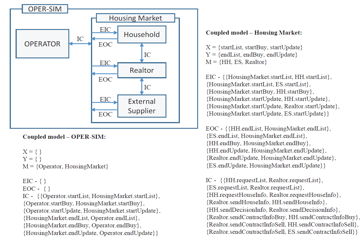
Next, the DEVS coupled model depicts the interaction between atomic models. Figure 1 illustrates the DEVS coupled model, showing the interaction of the components in our model. In the coupled model specification, X and Y specify the input and output of the coupled model, respectively, and M specifies the components of the coupled model. The external input coupling (EIC) specifies the information flow from the external model to the internal model of the coupled structure. Similarly, the external output coupling (EOC) specifies the outgoing information from the internal model of the coupled structure to the external model. Finally, the internal coupling (IC) depicts the couplings from a component output to a component input within the coupled structure. For example, in Figure 1, OPERATOR sends the market round signal to Household through the EIC of Housing Market. Having said that, OPERATOR and Housing Market resides at the same level, so their coupling is identified as IC.

Figure 1: DEVS coupled model of housing market model — **Figure 1.** DEVS coupled model of housing market model

Agent behaviors

To understand the model behavior, we illustrate three basic behaviors in the house transactions, which are list process, buy process, and update process. Our simulation iteratively executes the three behaviors over the simulated period.

We regard one iteration of these three processes as one simulation step, and we assume that one simulation step matches one month in terms of the real-world. Accordingly, we used the real-world values of the corresponding month as the value of the dynamic parameters. In addition, we adjusted the value of model parameters, which are not derived from the real-world, to the month scale by using the monthly validation data in the output validation.

List process

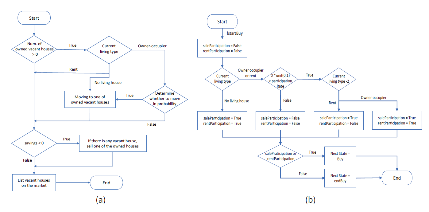
In the list process, the household agents and the external supplier agent list their houses to sell or to rent in the market. First, the agents decide whether to list their houses on the housing market. The following is the decision process of the household agents. Also, Figure 2 shows the flow chart of the list decision process.

Household agents identify vacant houses among their houses from the expiration of a rent contract or the purchase of a house.
Depending on the agent’s type of living, the household agents decide whether to move to a vacant house. This decision is required when there is at least one vacant house.
1. If the household agent has no living house, the agents move to one of the vacant houses. We assume that the house is randomly selected. The selected house is deleted from the list of vacant houses.
2. If the living type of the household is rent, the agents do not move to a vacant house.
3. If the living type of the household is owner-occupying, the agent decides whether to move, based on the parameter "HM: house moving rate". If the agent decides to move, then the agent initiates moving to one of the vacant houses. We assume that the house is randomly selected. The selected house is deleted from the list of vacant houses, and the previously occupied house is added to the list of vacant houses.
If the agent’s savings are negative and the list of vacant houses is empty, one randomly selected non-vacant house, among owned houses, is added to the list of vacant houses.
Finally, the agent sends the list of the vacant houses to the realtor agent for sale or rent.

The external supplier agent generates a number of vacant houses at each simulation time point, reflecting the real-world housing supply rate. The external supplier agent sends the list of vacant houses, including newly constructed houses, to the realtor agent for sale or rent. The realtor agent lists the houses gathered from the household agents and the external supplier agent in the market.

Buy process

In the buy process, the household agents purchase or rent a house for living or investment purpose. The household agents follow the below sequential decision-making process.

First, household agents determine whether to participate in the market. Then, household agents decide whether to purchase or rent by choosing their dealing type. Figure 2 represents the flow chart of this decision process. Instead of discrete agent categorization such as renters, first-time buyers, and buy-to-let investors of existing studies, household agents probabilistically determine the behavioral mode for market participation. The behavioral mode probability is affected by the agent’s economic and housing situations.
1. If the household agent has no living house, the agent must participate in the market. The dealing type is determined stochastically, using a Bernoulli trial with the parameter " SP: sale probability". In this case, the agent participates in the market as a renter or first-time buyer.
2. If the living type of the household is rent, the agent determines whether to participate in the market, according to the parameter "PP: market participate probability". If the agent decides to participate in the market, the dealing type is set to purchase. In this case, the agent participates in the market only as a first-time buyer. To simplify the model, the renter does not make another rental contract until the existing contract ends.
3. If the living type of the household is owner-occupying, the agent determines whether to participate in the market, according to the parameter "PP: market participate probability". If the agent decides to participate in the market, the dealing type is set stochastically by the parameter, " SP: sale probability". In this case, the agent participates in the market as a buy-to-let investor or home mover.
If the household agents decide to participate in the market, the agents determine their preferred house properties. Then, the determined preference properties are delivered to the realtor agent, and the realtor agent can send back a list of houses that satisfy the preferences. The following are the preference properties of the house, and we also specify the preference determination mechanisms for each preference property.
1. Region: The household agent uses real-world migration rate data to determine whether to migrate to another region. If the household agent decides to migrate, the region property is set to be the migration region. For instance, if the household agent in the capital region decides to migrate, the preferred region is the non-capital region. On the other hand, the household agent decides not to migrate, the region property is set to be the same as the current living region.
2. Maximum price: Formula (1) determines the upper limit of the price of the preferred house.
3. Minimum price : Formula (2) determines the lower limit of the price of the preferred house.
The realtor agent selects arbitrary Z houses, which satisfy the household’s preferences, from the listed houses on the market. Z is an integer parameter that can control the degree of information asymmetry in the market. Throughout this paper, we use ten as the value of Z. The realtor agent sends a brochure with the information for the selected houses, including their prices, to the household agents.

The household, who receives the brochure from the realtor agent, selects a house from the list by checking its financial affordability and quality.

If the household agent decides to purchase a house, Formula (3) is used to calculate the maximum affordable budget.

\[\begin{split} affordable\; budget\; purchase = WTP \times [min(amountLTV,\; amountDTI) + savings] \end{split}\]

\[(3)\]

Here, amountLTV is the maximum mortgage size limited by the LTV regulation.

If the house price satisfies the following conditions, the house is affordable.

\[affordable\; budget\; purchase \geq marketPrice + tax\; acquisition\]

\[(4)\]

Here, tax acquisition is the acquisition tax amount, and we follow the calculation from the Korean government.
If the household agent decides to rent a house, Formula (5) is used to calculate the maximum affordable budget. To cover "Jeonse" ³ in rental modeling, we add the savings term to the formula.

\[\begin{split} affordable\; budget\; rent = savings \times WTP + disposable\; income \div (\gamma_t/12) \end{split}\]

\[(5)\]

Here, disposable income is the disposable income of the household agent; \(\gamma_t\) is the conversion rate for converting the rent deposit to the rental fee at time \(t\).
If the house price satisfies the following conditions, the house is affordable.

\[affordable\; budget\; rent \geq marketPrice \times \Gamma_t\]

\[(6)\]

Here, \(\Gamma_t\) is the conversion rate for converting purchasing price to jeonse deposit at time \(t\).

If there is more than one affordable houses, the agent chooses the highest quality house as the transaction object. If there is more than one affordable houses of the same quality, the agent chooses the cheapest house as the transaction object.

Finally, the realtor agent mediates the contract between the buyer agent and the owner agent with the matched transaction object.

Update process

In the update process, the attributes of the household agents and the house objects are updated.

The household agent’s incomeWork and savings are updated first. The incomeWork varies according to the monthly inflation rate. In addition, the savings amount is updated by adding the disposable income. We assumed that the disposable income can be negative because of loan repayments or taxation.
If there is a terminated rent contract, the owner agent returns the rental deposit to the rentee household agent, and the rentee household agent vacates the house.

Next, we update the marketPrice attribute of all house objects according to the market preference. The marketPrice update consists of the price increment process and the price decrement process.

The price increment process applies to all house objects. Using the market preference value of houses with the same quality, if the preference value is above a certain preference threshold, the market price is increased by adding a parameterized increment amount adjusted by the inflation rate, in Formula (7).

\[marketPrice = marketPrice \times (1+ i_t + MP_u)\]

\[(7)\]

Here, \(MP_u\) is the rate for increasing market price; \(i_t\) is the inflation rate at time \(t\).
If the preference value is lower than a certain preference threshold, the market price is adjusted by only the inflation rate.

\[marketPrice = marketPrice \times (1 + i_t)\]

\[(8)\]

We set the preference value to be the exponential moving average (EMA) value of the transaction success rate of houses with the same quality.

The price decrement process only applies to the houses that failed in terms of transaction in the market (both unsold and not rented). Formula (9) specifies the market price of transaction failed houses.

\[marketPrice = marketPrice \times (1-MP_d)\]

\[(9)\]

Here, \(MP_d\) is the rate for decreasing market price. The price increment and the price decrement processes are two independent processes that are executed in turn.

Flow diagram

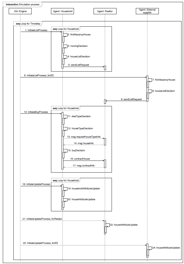
Figure 3 shows the flow diagram of the housing market model, including the list process, buy process, and update process. In every process, the household agents proceed in sequence and the order of agents varies randomly. Unlike the auction concept, the brochure concept does not have a mechanism to prioritize when multiple household agents want to buy the same house. To compensate for this weakness, we assume that the agent who goes through the process first preempts the desired house. Some agents do not monopolize the preemption benefits, because the order of the agents changes in each process.

Results

Output validation

Before starting our policy experiments, we took several steps to make a virtual housing market similar to the Korean housing market. It is easy to accept that even the same policy can have different effects depending on the target economic conditions. In other words, policy application cases in similar economic conditions give more accurate and helpful policy implications. In this regard, we used the Korean census data to set the initial characteristics of the household agents, and we used the actual economic values of Korea as model parameters that represent the economic environment of the model.

We alse conducted an output validation with the same intention (Manson 2003). We used the real-world house price index and house transaction volume data for this output validation. Because we used the census data of 2015, when we generated the initial household agents, it is natural that we set 2015 as the starting point of the sample period for the validation data. In addition, we set 2017 as the ending point of the sample period because there have been large policy changes in the Korean housing market since 2018.

**Table 3:** List of input parameters used in the housing market model
Type	Symbol	Name	Description	Default value (Source)	Calibrated value
Static	\(N_h\)	Household number	The number of household agents	2000	-
	\(N_r\)	Realtor number	The number of realtor agents	1	-
	\(N_h\)	External supplier number	The number of external supplier agents	1	-
	\(T\)	Simulation time	Max simulation run time (1 unit = 1 month)	36	-
	\(HS_c\)	Housing supply rate (capital)	Housing supply rate in the capital area	0.979 (Korea Appraisal Board)	-
	\(HS_{nc}\)	Housing supply rate (non-capital)	Housing supply rate in the non-capital area	1.065 (Korea Appraisal Board)	-
	\(D_m\)	Mortgage loan maturity	Maturity value of mortgage loans	120 (Korea Housing Finance Corp.)	-
	\(D_c\)	Credit loan maturity	Maturity value of credit loans	60	No
	\(QR\)	House quality resolution	Resolution value of house quality	10	No
	\(HM\)	House moving rate	Probability of moving to owned vacant houses	0.1	Yes
	\(PP_c\)	Market participate probability (capital)	Probability of market participation for households with residential house (capital)	0.007	Yes
	\(PP_{nc}\)	Market participate probability (non-capital)	Probability of market participation for households with residential house (non-capital)	0.002	Yes
	\(WTP\)	Willingness to pay	Maximum pay intention ratio of household	0.7	Yes
	\(SP\)	Sale probabilty	Probability of determining dealing type as purchase	0.3	Yes
	\(Z\)	Number of listed house in a brochure	Degree of information asymmetry in the market	10	No
	\(\alpha\)	EMA discount parameter	Discount parameter values in EMA (exponential moving average)	0.2	No
	\(K\)	Priority threshold	Threshold value of the house price increase process	0.35	Yes
	\(MP_u\)	Market price increase rate	Market price increase rate of houses	0.007	Yes
	\(MP_d\)	Market price decrease rate	Market price decrease rate of houses	0.2	Yes
	\(CR_q\)	Consumption rate	Consumption rate by income quintile ( \(q\) th quintile)	(Statistics Korea)	-
Dynamic	\(r_t\)	Interest rate	Interest rate of loan	(Bank of Korea)	-
	\(i_t\)	Inflation rate	Inflation rate calculated based on CPI index	(Statistics Korea)	-
	\(\Gamma_t\)	Jeonse-price exchange rate	Exchange rate of jeonse deposit to purchase price for housing	(Kookmin Bank)	-
	\(\gamma_t\)	Rent-jeonse exchange rate	Exchange rate of rental fee and jeonse deposit (monthly rental fee * 12 / deposit)	(Korea Appraisal Board)	-
	\(HT_{i,t}\)	House type proportion	Proportion of house type \(i\) (1: detached house, 2: apartment, 3: row house)	(Kookmin Bank)	-
	\(HP_{i,t}\)	House price per unit area	House price per unit area of house type \(i\) (1: detached house, 2: apartment, 3: row house)	(Kookmin Bank)	-
	\(RM_{c,t}\)	Region moving rate (capital)	Probability of non-capital migration of households living in the capital	(Statistics Korea)	-
	\(RM_{nc,t}\)	Region moving rate (non-capital)	Probability of capital migration of households living in the non-capital	(Statistics Korea)	-
	\(LTV_t\)	LTV regulation limit	Loan-to-value regulation limit	(Financial Services Commission)	-
	\(DTI_t\)	DTI regulation limit	Debt-to-income regulation limit	(Financial Services Commission)	-

Table 3 enumerates the calibrated parameter values, which are essentially abstract variables that are hard to be survey from the archived data. Mainly, these calibrated parameters are related to the preference and the utility of individual households. We calibrated these parameters through the design of experiments in a full factorial setting, and we selected values to capture the validation data through confidence intervals as in Figure 4. It should be noted that this experimental design was used for the calibration only, and this design is different from the experimental design in Table 4, which was aimed at testing the hypotheses with virtual experiments.

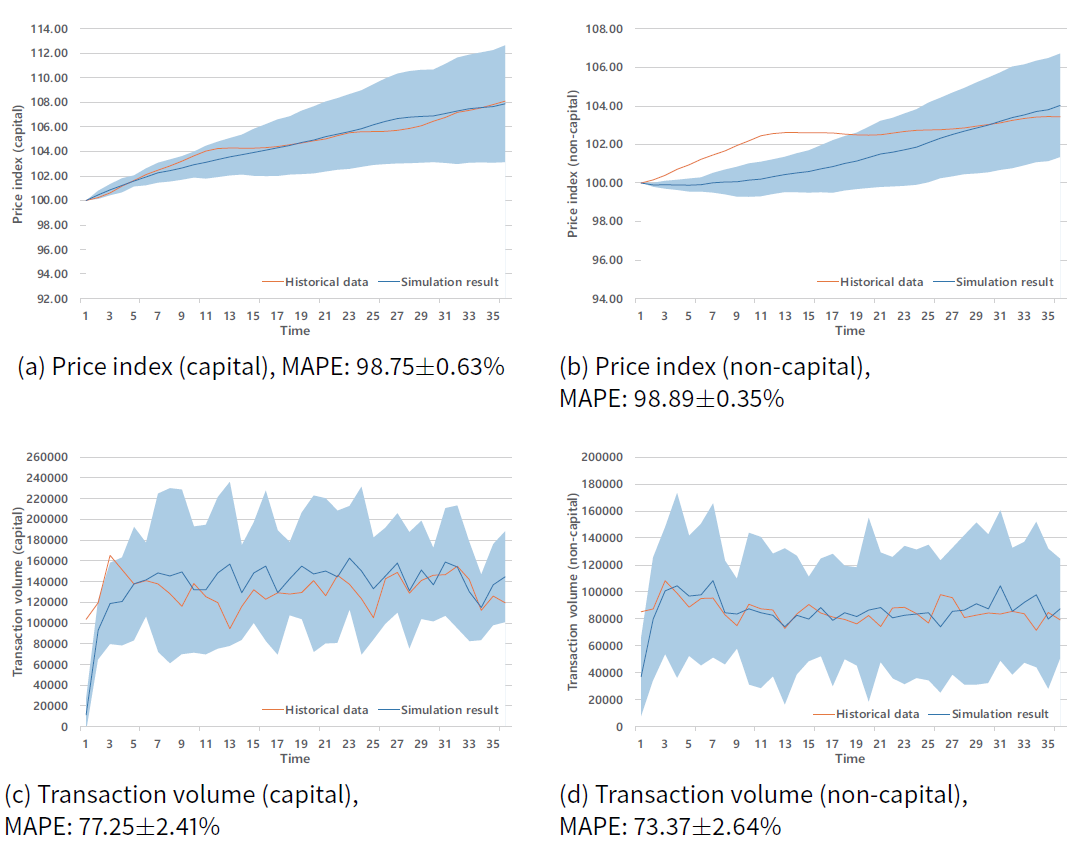
Figure 4: Comparison of the simulation results with historical data — **Figure 4.** Comparison of the simulation results with historical data

Figure 4 plots a comparison of the simulation output and the real-world data after the output validation. The simulation result is the average value of ten replications, and the colored area in the figure represents the 95% confidence interval of the simulation results. We also calculated the statistical fitness of the simulation results with the historical data, using the mean absolute percentage error (MAPE).

Based on Figure 4, we claim that the model is output validated with regard to the housing price index and transaction volume. Furthermore, the output validation result implies that the model is able to reproduce the following stylized fact. First, from the historical data plotted in Figure 4 (a) and Figure 4(b), we find that the capital region has a steeper rate of rising housing prices compared to the non-capital region. Similarly, the historical data plotted in Figure 4 (c) and Figure 4 (d) show that the capital region has higher transaction volume levels compared to the non-capital region.

Policy experiments

Our policy experiments were designed to identify the impact of changes in LTV and DTI limits on the housing market and individual households. Table 4 describes the experimental design of the policy experiments. We used both descriptive analysis and regression analysis to reflect the changes in LTV and DTI. Through the descriptive analysis, we investigated a single variable change of either LTV or DTI. The regression analysis revealed the joint influence of LTV and DTI on the markets and households. Formula (10) specifies the baseline model for the regression analysis.

\[Y_i = \alpha + \beta_1 \times LTV_i + \beta_2 \times DTI_i + \epsilon_i\]

\[(10)\]

\(LTV_i\) and \(DTI_i\) denote the limit value of LTV and DTI regulation in policy case i . \(\beta_1\) is the degree to which the dependent variable Y changes in reponse to changes in LTV regulation. Similarly, \(\beta_2\) is the degree to which the dependent variable Y changes in reponse to changes in DTI regulation. We used ordinary least squares (OLS) to estimate the equation.

**Table 4:** Experimental design of virtual experiments with macro-prudential polices
Variables	Variation case	Implication
Loan-to-value	\(\Delta\) (LTV) \(\sim\) uniform(-0.6, 0.1)	The value of \(\Delta\) (LTV) is added to the historical LTV setting of the sample period, in parallel
Debt-to-income	\(\Delta\) (DTI) \(\sim\) uniform(-0.6, 0.1)	The value of \(\Delta\) (DTI) is added to the historical DTI setting of the sample period, in parallel
Policy experiments	Number of policy variation cases	Number of repeat experiments
Descriptive analysis
- Single-variable cases	100 policy cases: varies each LTV or DTI respectively	10 replications on each case (100 \(\times\) 10 = 1000 simulations)
Regression analysis
- Joint-variable cases	200 policy cases: varies both LTV and DTI simultaneously	10 replications on each case (200 \(\times\) 10 = 2000 simulations)

Analysis of RQ1

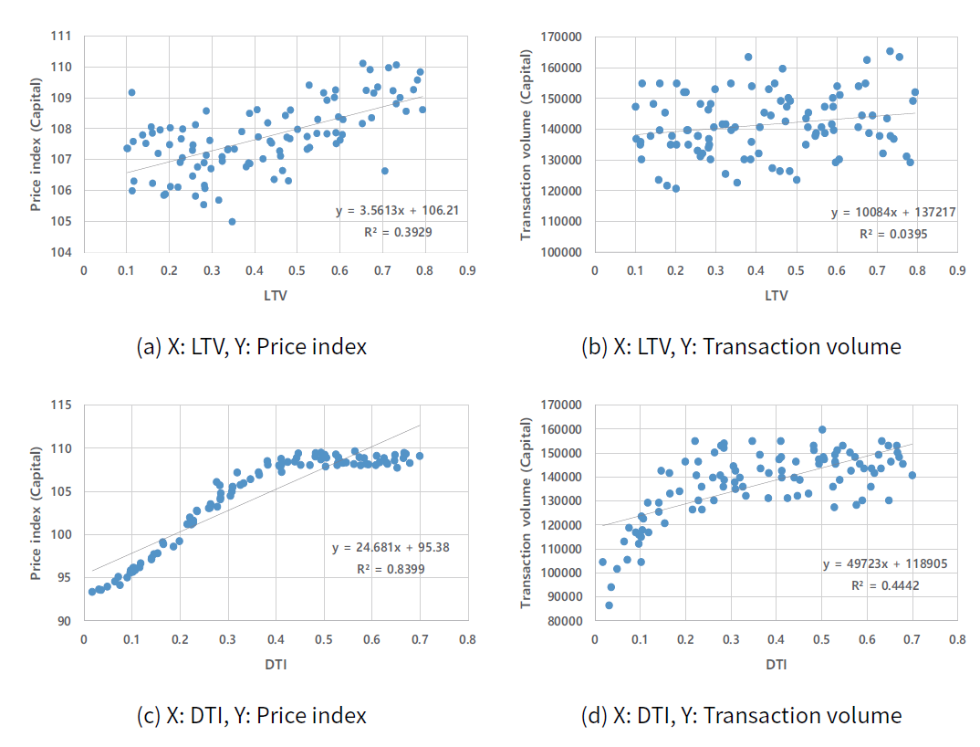
First, we investigated the impact of the LTV and DTI regulation changes on the housing market. We seleted the last simulation time-step housing index and the transaction volume as the dependent variables. Figure 5 shows the changes in the dependent variables when the values of LTV and DTI regulations are varied. The result indicates that tightening the LTV and DTI regulations decreases the housing price growth and the house transaction volume. This result is consistent with previous empirical studies, which investigated the impact of LTV and DTI regulation on the housing market (Crowe et al. 2013; Igan & Kang 2011; Jacome & Mitra 2015).

Table 5 shows the result of the regression analysis, through which we investigated the effects of each policy when both LTV and DTI regulations change simultaneously. Table 5 shows that the relaxation of LTV and DTI has a significantly positive impact on the housing price index. However, only the relaxation of DTI has a significantly positive impact on the transaction volume. In addition, we compared the magnitude of the impact from LTV and DTI between the capital region and the non-capital region. According to the comparison between column (a) and column (c) in Table 5, the changes in LTV have a similar magnitude of impact on both regions, while the impact of DTI changes has a stronger influence on the capital region. In other words, the LTV regulation has a consistent effect on the target market environment, whereas the effect of the DTI regulation varies depending on the target market environment.

Figure 5: Descriptive analysis of the effect macroprudential policies on housing market — **Figure 5.** Descriptive analysis of the effect macroprudential policies on housing market

**Table 5:** Regression analysis for the impact of LTV and DTI on housing market.
	Capital price index		Non-capital price index		Capital transaction volume		Non-capital transaction volume
	(a)	(b)	(c)	(d)	(e)	(f)	(g)	(h)
Constants	93.7578*** (103.1368)	95.0493*** (103.1368)	93.2159*** (100.3608)	94.1414*** (100.3608)	117080*** (134450)	123990*** (134450)	72116*** (81603)	77296*** (81603)
Macro-prudential policy
LTV	2.1257*** (0.4136)	-0.4476 (-0.0871)	2.1551*** (0.4193)	0.3097 (0.0603)	1058.7 (205.9991)	-12705 (-2472.2)	-4494.0 (-874.4358)	-14824 (-2884.4)
DTI	24.6372*** (4.6886)	20.9692*** (3.9713)	18.0201*** (3.4293)	15.3173*** (2.9150)	49670*** (9452.5)	29511** (5616.2)	34234*** (6515.0)	19105** (3635.8)
LTV ^* DTI		7.6428** (0.8904)		5.4808* (0.6385)		40879* (4762.5)		30679* (3573.2)
Observation	200	200	200	200	200	200	200	200
R-squared	0.8609	0.8642	0.8094	0.8123	0.3726	0.3824	0.3404	0.3506
Adj. R-squared	0.8595	0.8621	0.8074	0.8094	0.3662	0.3730	0.3337	0.3407

Notes: The table reports the estimation results of the regression analysis. The numbers denote the coefficient values of the estimation results. Numbers in parentheses denote standardized coefficient values. Estimates with ***, **, * denote statistical significance at the 1%, 5%, and 10% level, respectively.

Analysis of RQ2

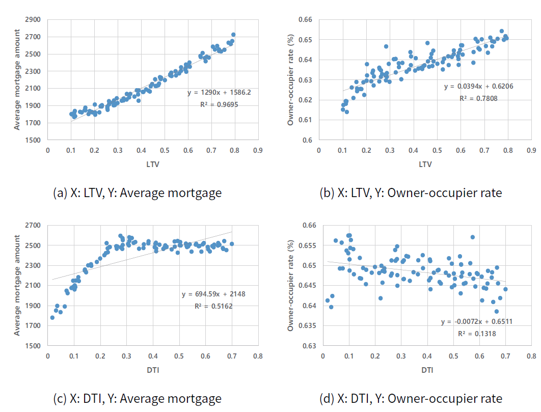
Next, we investigated the impact of the LTV and DTI regulation changes on the individual household. We used the last simulation time-step average mortgage amount and the owner-occupier rate as the dependent variables. As mentioned in the Introduction, we interpret the average mortgage amount as a quantitative proxy of the benefit, obtained from the mortgage. Furthermore, we interpret the owner-occupier rate as a distribution proxy of the benefit obtained from the mortgage.

Figure 6 shows the changes in the dependent variables when each of the LTV and DTI regulations is varied, respectively, and Table 6 summarizes the result of the regression, by which we investigated the effects of each policy when both LTV and DTI regulations change. The results show that the relaxation of both LTV and DTI regulations has a significantly positive impact on the average mortgage amount. These results are also consistent with the results of previous empirical studies, suggesting that LTV and DTI are effective policy instruments to lower the household debt (Crowe et al. 2013; Igan & Kang 2011; Jacome & Mitra 2015; Wong et al. 2011). However, only the relaxation of the LTV regulation leads to an increase in the owner-occupier rate. The relaxation of the DTI regulation has no significant effect on the owner-occupier rate in the housing market model.

**Table 6:** Regression analysis for the impact of LTV and DTI on households.
	Average mortgage amount		Lower-income class average mortgage amount		Owner-occupier rate		Lower-income class owner-occupier rate
	(a)	(b)	(c)	(d)	(e)	(f)	(g)	(h)
Constants	1434.6*** (2122.8)	1787.7*** (2122.8)	255.4183*** (267.2335)	256.0816**** (267.2335)	0.6248*** (0.6403)	0.6308*** (0.6403)	0.4994*** (0.5080)	0.5032*** (0.5080)
Macro-prudential policy
LTV	1068.3*** (207.8704)	364.2574*** (70.8769)	16.5624.0** (3.2227)	15.3498 (2.9653)	0.0329*** (0.0064)	0.0209*** (0.0041)	0.0207*** (0.0040)	0.0132** (0.0026)
DTI	529.8892*** (100.8408)	-501.2723*** (-95.3949)	11.5884 (2.2053)	9.6514 (1.8367)	-0.0003 (-0.0000)	-0.0178*** (-0.0034)	-0.0036** (-0.0000)	-0.0146* (-0.0028))
LTV ^* DTI		2091.0*** (243.6118)		3.9280 (0.4576)		0.0355*** (0.0041)		0.0224 (0.0026)
Observation	200	200	200	200	200	200	200	200
R-squared	0.7326	0.8221	0.0363	0.0363	0.6022	0.6281	0.1830	0.1906
Adj. R-squared	0.7299	0.8194	0.0265	0.0265	0.5981	0.6225	0.1748	0.1782

Notes : The table reports the estimation results of the regression analysis. The numbers denote the coefficient values of the estimation results. Numbers in parentheses denote standardized coefficient values. Estimates with ***, **, * denote statistical significance at the 1%, 5%, and 10% level, respectively.

Figure 6: Descriptive analysis of the effect of LTV and DTI policies on households — **Figure 6.** Descriptive analysis of the effect of LTV and DTI policies on households

Analysis of RQ3

Lastly, we investigated the impact of the LTV and DTI regulation changes on the lower-income class households. Figure 7 shows the effect of changes in LTV and DTI on the average mortgage amount and the owner-occupier rate of the lower-income class households. Table 6 reports the regression analysis result for the lower-income class. When we focused our analyses on the lower-income class households, the deregulation of LTV had a significant impact on increasing the average mortgage amount, and increasing the average mortgage amount leads to an increase in the owner-occupier rate of the lower-income class. On the contrary, the deregulation of DTI has no significant effect on the mortgage amount of lower-income class households.

Figure 7: Descriptive analysis of the effect of LTV and DTI policies on lower-income class households — **Figure 7.** Descriptive analysis of the effect of LTV and DTI policies on lower-income class households

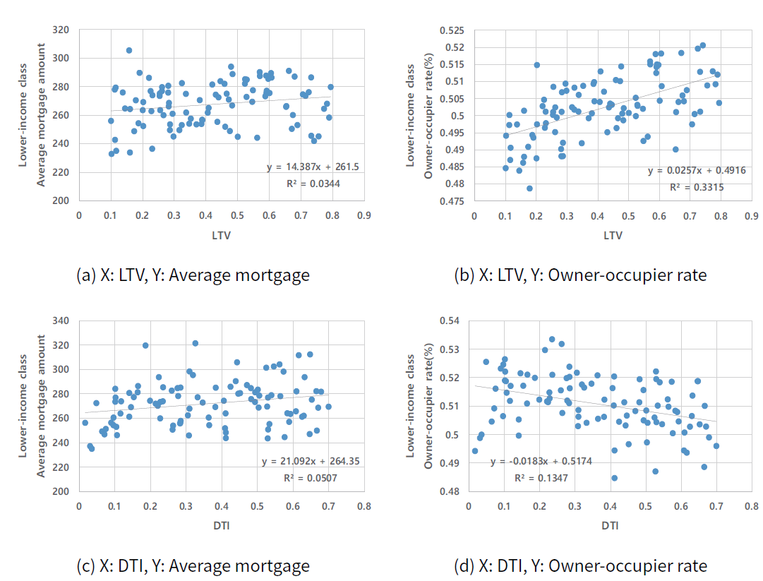
We conjecture that the underlying reason is the inherent characteristics of the DTI. Unlike the LTV, which is only influenced by the value of the collateral, the DTI is affected by the borrower’s income status. In other words, the same relaxation on the DTI regulation will dictate the lesser loan increment amount to the lower-income households and the higher loan increment to the higher-income households. This increment disparity will create more severe inequality in the housing market positions of the lower- and the higher-income households because of the greater demand across entire households on the housing market, and because of the increment in the house price. This result is well aligned with recent empirical studies, suggesting that the expansion of financial services adversely affects economic development (Arcand et al. 2015; Beck et al. 2007; Cecchetti & Kharroubi 2012) and income distribution (Park & Shin 2017). Furthermore, our result is in line with the study of Botta et al., which theoretically showed that increasing securitization in the financial system accelerates income and wealth inequality (Botta et al. 2019). Our result suggests one possible channel of the quantitative expansion of financial services causing wealth inequality, through mortgages.

Conclusion

This study introduces an agent-based model of the housing market with LTV and DTI interventions. Our model uses the brochure concept as a market mechanism, instead of the auction concept. This difference makes the proposed model suitable for modeling the inherent characteristics of the housing market. To enhance model reliability, we conducted output validation and structural validation to replicate the stylized facts of the previous empirical studies. Using the validated model, we investigated the impact of the LTV and DTI regulations on both macro and micro levels.

Our findings offer the following policy implications on the macro-prudential policies. First, the LTV regulation is a consistent policy instrument in the markets. However, the DTI regulation is a policy tool that has inconsistent effects depending on the markets. In this study, we did not verify which characteristics of the market influence the magnitude of the DTI regulation effect; we left that for future work. Second, the relaxation of both LTV and DTI regulations leads to an increase in the average mortgage amount, but only the relaxation of LTV leads to the alleviation of the housing distribution indicator. In other words, the trade-off relationship between the financial stability of households and the housing distribution only appears in the LTV regulation. Lastly, we showed that the lower-income class households are less likely to own a house under relaxed DTI regulations. This result supports a paradoxical argument that financial development accelerates wealth inequality.

For further research, using the model, we will identify the effect of the LTV and the DTI regulation changes on the economic variables that are difficult to observe in the real-world. For example, we will observe the wealth inequality of the households and the distribution of housing quality by the owner’s income status, through simulations. Additionally, we expect to see a combined effect of the LTV and DTI regulations with monetary policies and fiscal policies.

Acknowledgements

This work was supported by Institute of Information & Communications Technology Planning & Evaluation(IITP) grant funded by the Korea government(MSIT) (No.2018-0-00225).

Notes

In Jacome and Mitra’s words, the main goals of LTV and DTI regulation are to stem excessive credit growth and prevent a boom in house price (Jacome & Mitra 2015).
Gilbert et al. (2009) modeled a number of realtors to reflect these properties in their model.
Jeonse is a unique form of housing contract in the Korean housing market. See Shin and Kim (2013)'s work for details.

References

ARCAND, J. L.,

References

ARCAND, J. L., Berkes, E., & Panizza, U. (2015). Too much finance? Journal of Economic Growth, 20(2), 105–148. [doi:10.1007/s10887-015-9115-2]
AXTELL, R., Farmer, D., Geanakoplos, J., Howitt, P., Carrella, E., Conlee, B., & Palmer, N. (2014). An agent-based model of the housing market bubble in metropolitan Washington, DC. Whitepaper for Deutsche Bundesbank’s Spring Conference on “Housing Markets and the Macroeconomy: Challenges for Monetary Policy and Financial Stability.” May. [doi:10.2139/ssrn.2018375]
BAPTISTA, R., Farmer, J. D., Hinterschweiger, M., Low, K., Tang, D., & Uluc, A. (2016). Macroprudential policy in an agent-based model of the UK housing market. Bank of England working papers 619, Bank of England. [doi:10.2139/ssrn.2850414]
BECK, T., Demirgüç-Kunt, A., & Levine, R. (2007). Finance, inequality and the poor. Journal of Economic Growth, 12(1), 27–49. [doi:10.1007/s10887-007-9010-6]
BERNANKE, B. S. (2011). The effects of the great recession on central bank doctrine and practice. The B.E. Journal of Macroeconomics, 12(3) [doi:10.1515/1935-1690.120]
BOTTA, A., Caverzasi, E., Russo, A., Gallegati, M., & Stiglitz, J. E. (2019). Inequality and finance in a rent economy. Journal of Economic Behavior & Organization. Available online 17 April 2019. [doi:10.1016/j.jebo.2019.02.013]
BRAUN-MUNZINGER, K., Liu, Z., & Turrell, A. (2016). An agent-based model of dynamics in corporate bond trading. Bank of England working papers 592, Bank of England. [doi:10.2139/ssrn.2766368]
CECCHETTI, S. G., & Kharroubi, E. (2012). Reassessing the impact of finance on growth. BIS Working Paper, No. 381.
CHRISTENSEN, I., & others. (2011). Mortgage debt and procyclicality in the housing market. Bank of Canada Review, 2011(Summer), 35–42.
CROWE, C., Dell’Ariccia, G., Igan, D., & Rabanal, P. (2013). How to deal with real estate booms: Lessons from country experiences. Journal of Financial Stability, 9(3), 300–319. [doi:10.1016/j.jfs.2013.05.003]
CUSSEN, M., O’Brien, M., Onorante, L., O’Reilly, G., & others. (2015). Assessing the impact of macroprudential measures. Central Bank of Ireland.
DOSI, G., Fagiolo, G., & Roventini, A. (2010). Schumpeter meeting Keynes: A policy-friendly model of endogenous growth and business cycles. Journal of Economic Dynamics and Control, 34(9), 1748–1767. [doi:10.1016/j.jedc.2010.06.018]
FULLER, G. W., Johnston, A., & Regan, A. (2020). Housing prices and wealth inequality in western europe. West European Politics, 43(2), 297–320. [doi:10.1080/01402382.2018.1561054]
GE, J. (2013). 'Who creates housing bubbles? An agent-based study.' International Workshop on Multi-Agent Systems and Agent-Based Simulation, Berlin Heidelberg, Springer, pp. 143–150. [doi:10.1007/978-3-642-54783-6_10]
GEANAKOPLOS, J., Axtell, R., Farmer, J. D., Howitt, P., Conlee, B., Goldstein, J., Hendrey, M., Palmer, N. M., & Yang, C.-Y. (2012). Getting at systemic risk via an agent-based model of the housing market. American Economic Review, 102(3), 53–58. [doi:10.1257/aer.102.3.53]
GELAIN, P., Lansing, K. J., & Mendicino, C. (2013). House prices, credit growth, and excess volatility: Implications for monetary and macroprudential policy. International Journal of Central Banking, 9(2), 219-276. [doi:10.2139/ssrn.2258465]
GILBERT, N., Hawksworth, J. C., & Swinney, P. A. (2009). An agent-based model of the English housing market. AAAI Spring Symposium: Technosocial Predictive Analytics, 30–35.
HIMMELBERG, C., Mayer, C., & Sinai, T. (2005). Assessing high house prices: Bubbles, fundamentals and misperceptions. Journal of Economic Perspectives, 19(4), 67–92. [doi:10.3386/w11643]
IACOVIELLO, M. (2005). House prices, borrowing constraints, and monetary policy in the business cycle. American Economic Review, 95(3), 739–764. [doi:10.1257/0002828054201477]
IGAN, D., & Kang, H. (2011). Do loan-to-value and debt-to-income limits work? Evidence from Korea. IMF Working Papers, 1–34. [doi:10.5089/9781463927837.001]
JACOME, L., & Mitra, S. (2015). LTV and DTI: Going Granular. IMF Working Paper 15/154.
KANNAN, P., Rabanal, P., & Scott, A. M. (2012). Monetary and macroprudential policy rules in a model with house price booms. The BE Journal of Macroeconomics, 12(1). [doi:10.1515/1935-1690.2268]
KUTTNER, K., Shim, I., & others. (2012). 'Taming the real estate beast: The effects of monetary and macroprudential policies on housing prices and credit.' In Heath, A., Packer, F., & Windsor, C. (Eds), Property Markets and Financial Stability. Sydney: Reserve Bank of Australia, 231–259.
LALIOTIS, D., Buesa, A., Leber, M., & Población Garcı́a, F. J. (2019). An agent-based model for the assessment of LTV caps. Working Paper Series 2294, European Central Bank. [doi:10.1080/14697688.2020.1733058]
LAMBERTINI, L., Mendicino, C., & Punzi, M. T. (2013). Leaning against boom–bust cycles in credit and housing prices. Journal of Economic Dynamics and Control, 37(8), 1500–1522. [doi:10.1016/j.jedc.2013.03.008]
MANSON, S. (2003). 'Validation and verification of multi-agent models for ecosystem management.' In Hanssen, M. (Ed), Complexity and Ecosystem Management: The Theory and Practice of Multi-Agent Approaches, Edward Elgar, Northampton, pp. 63–74.
MENDICINO, C., & Punzi, M. T. (2014). House prices, capital inflows and macroprudential policy. Journal of Banking & Finance, 49, 337–355. [doi:10.1016/j.jbankfin.2014.06.007]
PARK, D., & Shin, K. (2017). Economic growth, financial development, and income inequality. Emerging Markets Finance and Trade, 53(12), 2794–2825. [doi:10.1080/1540496x.2017.1333958]
SHIN, H. S., Kim, S.-J., & others. (2013). Financing growth without banks: Korean housing repo contract. 2013 Meeting Papers, 328.
TESFATSION, L., & Judd, K. L. (2006). Handbook of Computational Economics: Agent-Based Computational Economics (Vol. 2). Amsterdam: Elsevier.
TURRELL, A. (2016). Agent-based models: Understanding the economy from the bottom up. Bank of England Quarterly Bulletin, Q4.
WONG, T., Fong, T., Li, K.-f., & Choi, H. (2011). Loan-to-value ratio as a macroprudential tool-Hong Kong’s experience and cross-country evidence. Systemic Risk, Basel III, Financial Stability and Regulation. [doi:10.2139/ssrn.1768546]
ZEIGLER, B. P. (1984). Multifacetted Modelling and Discrete Event Simulation. Academic Press Professional, Inc.