An Agent Based Model of a Thinly Traded Land Market in an Urbanizing Region

Introduction

Modeling human decisions is one of the biggest challenges in agent-based models (Dou et al. 2020; Filatova et al. 2013; Schülze et al. 2017). As part of the continuous endeavor to address this challenge, many researchers have contributed to consolidating the economic foundations of land-use change decisions both at a micro (Ettema 2011; Filatova 2015; Koch et al. 2019; Magliocca et al. 2011, 2014; Parker & Filatova 2008)and macro levels (Dou et al. 2020), as reviewed by Groeneveld et al. (2017). These developments have substantially narrowed the gap between out-of-equilibrium agent-based simulation models and equilibrium-based economic models (Wrenn & Irwin 2015). In this paper, we extend these advances by transforming the recently developed static model of thinly traded land market (Chen et al. 2017) into a multi-period agent-based land use model. We also extended the thinly traded land market model to include open space amenities. This line of research is particularly important as it provides deeper understanding of the economic incentives behind land use change decision and can help to consolidate the human dimension in the application of agent-based models to a broad range of human-environment systems (Manson et al. 2020; Schülze et al. 2017; Tang & Yang 2020; Wallentin 2017).

The thinly traded land market model (Chen et al. 2017; Chen 2020) differs from existing models. In particular, it allows land demand (supply) to decrease (increase) over the urban-rural gradient. This condition of spatially varying market competition systematically affects households’ location decisions and landowners land conversion decisions.

Furthermore, early urban economic models of household location choice and land use decisions are based on spatial equilibrium conditions. Competition for scarce locations generates new prices that can fully offset the advantages or disadvantages associated with a location and thus households may have no incentive to relocate (e.g. Alonso 1964; Capozza & Helsley 1989; Roback 1982). These conditions provide a static representation of land use that reflects spatial competition over the long-term equilibrium. This description however, ignores the short-term out-of-equilibrium adjustments made by individual households and landowners that eventually lead to the equilibrium. Parker & Filatova (2008) are the first to propose that household bid prices in agent-based models should depend on market competition conditions, that is, the relative number of buyers and sellers, which they subsequently apply to their later work. For instance, they (Filatova 2015; Parker & Filatova 2008) assume that household bid prices are higher (lower) than sellers’ ask price if the aggregate number of buyers is higher than the number of parcels in the region. Indeed, Magliocca et al. (2011, 2014, 2018) allow this market competition measure change among bidding households.

Here, by developing an agent-based model based on the thinly traded land market model, we assume that market competition conditions can change from parcel to parcel depending on the number of buyers and the number of similar parcels available. The market competition condition is also affected by both the distance to the urban center and the presence of open space amenities. This spatial variation in market competition conditions and the consequent spatial differences in bargaining power are critical to interaction modeling between household spatial competition and the price pattern formation.

We need to add that the variation in land use pattern in this paper arises as a result of this line of reasoning in the thinly traded land market model: i.e., as distance to urban areas increases, more vacant land is available and fewer households compete for more distant locations. Consequently, landowners set a lower reserve price and bidding households bid lower on more distant locations. All else being equal, if the bid price for a parcel is lower, a household can retain a larger budget for the consumption of other goods. In this way, the household’s optimal location choice is directly affected by spatially differentiated bid prices and competition among households, resulting in a pattern of scattered development.

Using this model set-up and assuming exogenous population growth over time, we simulate the evolution of land rents, income and land-use patterns in a growing urbanizing area. We find that scattered development can emerge as the result of market competition for land become more limited over the urban-rural gradient as predicted in the static analysis of Chen et al. (2017), but that it disappears as the region becomes more populated and the competition for land increases. Our results also show that the intensity and persistence of the scattered development vary systematically with key economic parameters of the model. Specifically, the simulation of this agent-based model can replicate many stylized facts. For instance, higher transportation costs and faster rates of in-migration decreasing the relative amount of scattered development and reducing its persistence over time.

Finally, this paper makes a methodological contribution by offering one possible way to bridge the agent-based land-use models with spatial equilibrium models of urban economics. If the number of households competing for each parcel becomes very large, households bid their maximum willingness to pay and so there is no advantage to locating farther away. Under these conditions, the model reproduces an outward pattern of contiguous land development as predicted by standard spatial equilibrium models of urban economics. On the other hand, if the number of competing bidders on each parcel equals one, then it becomes a bi-lateral negotiation model as in Parker & Filatova (2008).

The rest of the paper is structured as follows. In Section 2, we provide a description of the model setup. Section 3 discusses the results and Section 4 concludes the paper.

Model Description

Overview

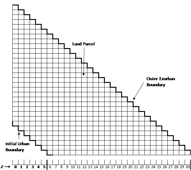
The model is implemented on a two-dimensional spatial grid comprised of equal area cells. Following monocentric land-use models in urban economics (Alonso 1964), all employment opportunities are concentrated at a fully developed urban center lying in the lower left corner. The boundary of this urban center is labeled as “initial urban boundary” in Figure 1. To focus on the urbanization process in sub-urban and exurban areas, we focus on the new development beyond this initial urban boundary. As new development fills up the parcels adjacent to this initial boundary, the urban boundary will gradually expand. We impose an “outer exurban boundary” (see Figure 1) that is sufficiently far away from the initial urban boundary, so that it is unlikely to affect the household location decisions.

Land parcels are represented by equal-sized cells of the grid. The region in the baseline model extends to a \(31 \times 31\) grid, which corresponds to roughly a maximum of one-hour commute to the initial urban boundary. In the initialization stage, land parcels are differentiated only by their Manhattan distance to the urban center \(z\). For example, a land parcel with coordinates \((x, y)\) relative to the origin (urban center) has distance \(z = |x|+|y|\). Under this definition of distance, the number of substitutable parcels (\(M\)), the number of parcels with the same distance (\(z\)) to urban center, increased naturally with distance because \(M(z) = z+1\). This allows us to build in the reality that the amount of developable land increased with distance to urban areas.

There are two types of economic agents: landowners and households. A landowner chooses the reserve price for the parcel, in order to maximize its expected payoff. Households are potential renters of the land parcels. Depending on their role in land market, households are further divided into three types: new migrants, relocating residents and non-relocating residents. New migrants are households outside the region and considering whether to move into the region and rent a land parcel. Existing residents in the region are migrants that choose to reside in the region in some previous period. Ninety-five per cent of the existing residents in each period are randomly selected to remain in their residing locations. These residents are called non-relocating residents. The remaining five per cent of residents are called relocating households. We assume that land for the relocating households is on the rental market along with other available land parcels. Relocating households enter the market and compete with the new migrants. Denote by \(N_{t}\) the total number of households actively looking to rent a parcel in period \(t\), which includes both new migrants and relocating households.

The number of competing bidders is derived from the income distribution of households. The cumulative (probability) distribution function (CDF) of household incomes is denoted by \(F(Y)\). \(Y_{min}(z,A)\) denoted the minimum income necessary to afford a parcel at distance \(z\) and with associated amenity \(A\) (see Section 2.5 and Equation 3 for details). Given \(Y_{min}(z,A)\), both the renters and sellers can calculate the probability a household with income randomly selected from the distribution \(F(Y)\), exceeding this minimum income level, i.e., \(Prob(Y>Y_{min}(z,A)) = 1-F(Y_{min}(z,A))\). Given that there were \(N_{t}^{0}\) households actively searching for locations, the expected number of competing households on a parcel with distance \(z\) in period \(t\) is calculated as:

\[N_{t}(z) = N_{t}^{0}[1-F(Y_{min}(z,A))] \]

\[(1)\]

where \(F(.)\) is the cumulative probability function (CDF) for household income distribution. To simplify this notation, we suppress the subscript \(t\) to \(N(z)\). The expected number of competing households (\(N(z)\)) affects households’ bidding strategy and landowners’ choice of reserve price (see Section 2.5 for details). Because the minimum income \(Y_{min}(z,A)\) increases monotonically with distance \(z\), \(N(z)\) was decreases in \(z\). Land parcels therefore differ in the expected number of competing households \(N(z)\). This builds in the stylized fact that land demand decreases over the urban-rural gradient. Because the minimum income \(Y_{min}(z,A)\) monotonically decreases with amenity \(A\) (see ), \(N(z)\) increases in \(A\). Finally, as households migrated into the region and land development occur, land parcels also differ in the level of open space amenity (\(A\)), that is, the percentage of un-occupied land among the neighboring parcels.

Renter’s behavior

It is worth noting that all households are modelled as renters because this simplifies the relocation decision by avoiding the resale of existing properties. Both the new migrants and the relocating households searching for all possible locations,¹ form optimal bids and try to find the best location that maximizes their utility \(U(C,L,A)\). Household utility is a function of numeraire good consumption (\(C\)), a fixed amount of land (\(L=1\)) with varying levels of open space amenity (A). Open space amenity (\(A\)) of a parcel is defined as the percentage of undeveloped parcels among the eight-connected parcels in its Moore neighborhood.

Renters are constrained by their income (\(Y\)), which is assumed to be randomly distributed with a cumulative distribution function denoted by \(F(Y)\). Income distribution is public information to all households and landowners. The household’s total expenditure on land rent (\(R\)), numeraire good consumption (\(C\)) and travel costs (\(T\)) should not exceed its income \((Y): R + C +T(Y,z) \leq Y\). The travel cost is assumed to increase with travel distance (\(z\)) and the opportunity cost of travel time which is proportional to income (\(Y\)).

A renter decides whether to migrate into the region as follows: If a renter chooses to stay outside of the region, she receives the reservation utility \(U_{0}\)from consuming a reservation level of numeraire good \(C_{r}^{0}\). If a renter chooses to migrate into the region, she needs to rent a land parcel in the region. The land parcel is characterized by the distance \(z\) to urban center and the amount of open space amenity \(A\). For a renter to reside on a land parcel in the region, her wellbeing should be at least as good as staying outside the region. That is, \(U(C,1,A) \geq U_{0}\). Denote by \(C_{r}\) the reservation consumption, or the minimum consumption required for the household to reside on that parcel. This reservation consumption can be defined as:

\[U(C_{r}(A),1,A)=U_{0} \]

\[(2)\]

Because \(C_{r}(A)\) is the minimum consumption level that makes the household indifferent to staying outside the region, the maximum willingness to pay (WTP) for the land parcel can be derived from the budget constraint as \(V(A)=Y-C_{r}(A)-T(Y,z)\).

Imagine a household choosing between two parcels located at the same distance from the urban center but differing in the open space amenities (\(A_{1}<A_{2}\)). Because both numeraire good and open space amenities are normal goods (\(\frac{\partial U}{\partial C} > 0\),\(\frac{\partial U}{\partial A} > 0\)), \(C_{r}(A_{1})>C_{r}(A_{2})\) (see Equation 2 and Roback (1982)) and the household income and travel costs are the same, the difference in maximum WTP for the two parcels is given by \(V(A_{2})-V(A_{1})=C_{r}(A_{1})-C_{r}(A_{2})\), which is determined by the differences in amenities. For simplicity, we denote the willingness to pay for amenities by \(W(A)\), and assume it increases linearly with the amenity \(A: W(A)= C_{r}^{0}-wA\), where \(w\) is a constant. That is, the higher the open space amenity (\(A\)), the more consumption the household is willing to sacrifice (\(C_{r}(A)\) decreases) and the higher the rent the household is willing to pay. Thus, the parcel value can be rewritten as:

\[V=Y-C_{r}^{0}-T(Y,z)+wA \]

\[(3)\]

A parcel with a positive value (\(V>0\)) is called an affordable parcel for the household. The minimum income that ensures \(V \geq 0\) is denoted as \(Y_{min}(z,A)\). This is also the minimum income to afford the reservation consumption at location \(z\). Because the reservation consumption is lower on parcels with open space amenities, the minimum income \(Y_{min}(z,A)\) monotonically decreases in \(A\). Because travel costs (\(T(Y,z)\)) increase with distance (\(z\)), the minimum income \(Y_{min}(z,A)\) monotonically increases with distance \(z\).

A household searches and bids on all affordable parcels. The optimal bid function \(b(V)\), the relation between the bid (\(b\)) and private value (\(V\)), is derived using a first price sealed-bid auction model (Krishna 2010). This household maximizes the expected surplus from winning this parcel. The surplus (\(V-b(V)\)) is the difference between the household value (\(V\)) of the parcel and the bid value (\(b\)) it would actually pay if it wins. This trade surplus is only realized if the household wins the auction. Thus, the household’s optimal bidding strategy solves:

\[max_{b(V)} [V-b(V)] H(b^{-1}) \]

\[(4)\]

where \(H(∙)\) is the probability that the household’s bid \(b(V)\) wins at least one of \(M\) identical parcels at location \(z\). Because the \(M\) parcels at location \(z\) are complete substitutes and \(N\) bidders are competing, household cares only about whether “it wins one of the \(M\) parcels” or “none of them”. Thus, the probability of winning given a bidding strategy \(b(.)\) is given by:

\[H(b^{-1})=1-[1-G^{N-1}(b^{-1})]^M \]

\[(5)\]

The bidding value is denoted as \(\beta=b(V)\). This implies that \(V(\beta)=b^{-1}(\beta)\). \(G(V)\) is the cumulative distribution function for household’s private value (\(V\)) of the parcel, which is derived from the income distribution \(F(Y)\). The second term on the right-hand side gives the probability of winning none of the \(M\) parcels.

Given the reserve price set by the landowner, the solution for the optimization problem in Equation 4 gives the optimal bid function \(b(∙)\) (Krishna 2010 p. 21):

\[\beta=b(V,r,M,N)=r \frac{H(r)}{H(V)} +\frac{1}{H(V)}\int_{r}^{V}yh(y)dy \]

\[(6)\]

where \(h(y)=\frac{\mathrm{dH(y)}}{\mathrm{d}y}\).

This optimal bid function depends not only on the household’s value of the parcel \(V\), but also on the expected number of competing households \(N\), the number of substitutable parcels \(M\), the reserve price, as well as the open-space amenity \(A\) of the parcel.

Seller’s behavior

Landowners optimally choose their reserve prices \(r\) to maximize their expected payoff. The formulation of this optimization problem is adapted from Krishna (2010 pp. 21–25):

\[\max_{r} \quad N(z)E[H(V)b(V)]+G(r)^{N(z)} r_{a} \]

\[(7)\]

The landowners’ expected payoff is defined to be the probability weighted sum of the expected payment: expected payment when the auction succeeds and the expected payment when the auction fails. If the land is successfully sold through auction, the expected bid price from one competitor is \(E[H(V)b(V)]\). There are \(N(z)\) competitors. Thus, the expected payment from a successful auction is the product of the two, as represented by the first term in Equation 7. If the auction fails, the landowner receives the agricultural payment \(r_{a}\). This occurs when all the bids are less than the reserve price. This is represented in the second term in Equation 7.

Market transaction

Households submits a bid for each affordable parcel. On each parcel, the bidder with the highest bid is identified. If a household has multiple winning bids exceeding the owner’s reserve price, it chooses the parcel that generated the highest surplus \(V-b(V)\). For the remaining parcels that the household wins, the bidder with the second highest bid is picked. This process continues until no bidder wins multiple parcels. At the end of this procedure, if the winning household’s bid is higher than the reserve price of the landowner, the winning household becomes the resident on the parcel and the land converts to residential use. The incumbent residents who loose in the auction on their resident land parcel are assumed to move out of the region.² Once a household wins a parcel and chooses a location, it is obligated to pay the bid submitted to the landowner. In other words, households are not allowed to renegotiate their bids within the same time-period as this would be in conflict with the interest of the landowner, whose expected payoff increases with \(N(z)\) as seen in Equation 7.

In this model, migration continues as long as the utility from residing in the region exceeds the utility from residing in the rest of the world. We acknowledge the existence of moving and search costs in the household location process. We therefore assume that migration is a gradual rather than an instantaneous process. In each period, a fixed number of potential new migrants is randomly selected to make the migration decision. As relocating households participate in the auctions, they update their bids under the new market conditions. Over time, this gradual adjustment in migration increases the competition for land, reduces the bargaining power of households, and diminishes the trade surplus from more distant parcels.

In this model, a spatial equilibrium is not reached instantaneously in each time-period. Over time, however, as the number of residents increased, the number of relocating residents increased accordingly. This process increased the competition for land and is the fundamental driving force behind the eventual convergence to the spatial equilibrium land-use pattern in the urban economics literature.

Simulation details

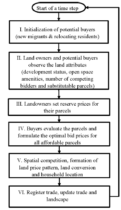
Figure 2 illustrates the sequence of processes in this model. Each time step starts with the initialization of the potential renters, which includes new migrating households and relocating residents (box I, Figure 2). Both renters and landowners then form an expectation of competition they face on each parcel (box II, Figure 2). After this, landowners formulate reserve prices and the renters formulate bid prices according to the first price sealed-bid auction theory (box III and IV, Figure 2). Landowners then rent their land to the highest bid if it exceeds the reserve price. Agricultural land is converted to residential use. Households choose the location that maximizes trade surplus. This process ensures that households’ spatial competition is simultaneously effecting and affected by land price patterns (box V, Figure 2).

Model Calibration

We use secondary data to calibrate the demand- and supply-side parameters of the model. The demand-side parameters of the model include fixed travel cost \(t_{0}\) per unit of distance, opportunity time cost \(t_{1}\) per unit of income per unit of distance, the reservation consumption level \(C_{r}^{0}\), and the income distribution \(F(Y)\).

Table 1: Variable descriptions. Note: The types include migrant, relocating resident and non-relocating resident.

Variable	Brief Description	Value
I. Land Parcel
\(z\)	Distance to Urban Area	\(\{1, 2, \dots 31\}\)
\(A(z)\)	Amount of Open Space Amenity	\(\{0, \frac{1}{8}, \frac{2}{8}, \dots 1\}\)
\(M(z)\)	Number of Substitutable Parcels	\(\{1, 2, \dots 31\}\)
\(N(z)\)	Number of Bidders on a Parcel
II. Households
Type	New Migrant, Relocating and Non-Relocating Residents	See Section 2.5
\(Y\)	Household Income	Lognormal
\(Y_{min}(z)\)	Minimum Income to Afford Parcel at Distance \(z\)
\(V(z,Y)\)	Household Private Value of a Parcel
\(U\)	Utility
\(L\)	Land Consumption	\(1\)
\(C_{r}^{0}\)	Reservation Consumption of the Numeraire Good
\(c_{0}\)	Fixed Reservation Consumption	\(5.9\)
\(c_{1}\)	Marginal Effect of Income on Reservation Consumption	\(0.3\)
\(T\)	Household Transportation Cost per Unit of Distance
\(t_{0}\)	Travel Cost per Unit Distance Independent of Income	\(0.19\)
\(t_{1}\)	Marginal Travel Cost per Unit Distance for Income	\(0.01\)
\(\beta = b(V)\)	Bid and Bid Function
III. Landowner
\(r(z)\)	Reserve Price
\(r_{a}\)	Agricultural Land Rent	\(16.32\)
IV. Market
\(F\)	CDF of Income Distribution	Lognormal
\(f\)	PDF of Income Distribution	Lognormal
\(G\)	CDF of the Parcel Value	Lognormal
\(g\)	PDF of the Parcel Value	Lognormal
\(N_{0}\)	Number of New Migrants Each Period	\(30\)

Reservation consumption is assumed to increase with income \(C_{r}^{0}=c_{0}+c_{1} Y\), calibrated using the 2010 consumer expenditure survey data (Bureau of Labor Statistics). We estimate a linear relationship between the average annual expenditure on goods and services (excluding housing and transportation expenditures) and after-tax income: \(C_{r}^{0}=c_{0}+c_{1}Y\). The ordinary least square method generates estimates \(c_{0}=5.9\) and \(c_{1}=0.3\). The fixed travel cost \(t_{0}\) per unit of distance is calibrated using the average transportation expenditure which is about \(13,697\) dollars according to the 2010 Consumer Expenditure Report. The opportunity cost of time, \(t_{1}Y\), is proportional to the household income. One-hour commuting time per day leads to an opportunity cost of \(\frac{1}{8}\) the household income. We calibrate the benchmark value for \(t_{1}\) using the ratio between the calibrate travel time for one parcel and the total annual working time. The former is calculated assuming an average speed of 50 miles per hour. This is calculated assuming the average exurban household works eight hours a day, five days a week and a total of 50 weeks a year. In addition, we assume that the fuel price is \(2.32\) dollars per gallon, which is approximately the oil price in 2010, and an average car travels 25 miles per gallon. This generates travel cost parameters with benchmark values of \(t_{0}=0.19\) and \(t_{1}=0.01\).

The parameters for the log-normal income distribution function \(F(Y)\) are calibrated using maximum likelihood estimation based on household counts by income categories for all non-metropolitan counties in the 2010 U.S. Census. \(\mu\) and \(\sigma ^ {2}\) respectively denote the expectation and variance of the log of income. The estimation yields were \(\mu=3.8024\) and \(\sigma=0.9591\). We also require that the income of a migrant needs to exceed the minimum income level for at least one parcel in the region. If the random draw of income falls below this value, we replace it with another draw until it rises above it.

The preference to open space amenities is calibrated based on McConnell & Walls (2005) value of open space. We assume that open space amenity surrounding the parcel increase the private value of the land parcel by \(1,000\) dollars McConnell & Walls (2005 p. 32). Therefore, in Equation 3, we set \(w=1\) (thousand dollars). The agricultural rent \(r_{a}\) is calibrated using the 2010 average cropland cash rent (\(102\) dollars per acre) in the U.S. (United States Department of Agriculture (USDA) 2016).

Results and Discussions

The main focus of this paper is to examine how the introduction of thinly traded land market theory affects simulated land use patterns. In particular, spatially varying market competition and open space amenities significantly affect the intensity and persistence of land use pattern. To facilitate this discussion, we quantify the intensity and persistence of scattered development as follows.

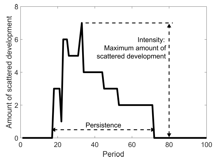
Scattered development occurrs if a parcel is developed at distance \(z_{1}\) while a parcel at a closer location \(z_{2}\) remains undeveloped, i.e., there is an undeveloped parcel at a distance \(z_{2}\), when a parcel at a more distant location \(z_{1}\) (\(z_{1}\)>\(z_{2}\)) is developed. The parcel at distance \(z_{1}\) is called a scattered parcel. The number of scattered parcels is referred to as the amount of scattered development. This changes from period to period. The intensity of scattered development is the maximum amount of scattered development over all simulation periods. The persistence of scattered development is the difference between the first period that scattered development appears and the first period that scattered development disappears.

Figure 3 illustrates the calculation of the intensity and persistence of scattered development. The simulation period is plotted along the x-axis and the amount of scattered development is shown along the y-axis. The amount of scattered development generated in a simulation with 100 periods is plotted as a solid line. Initially, there is no scattered development. Scattered development emerges in period 19 and begins to increase. After reaching its maximum value of seven, the amount of scattered development diminishes until it disappears in period 72. In this illustrative example, the intensity of scattered development equals seven, the maximum amount of scattered development. The persistence was \(54 (=72-19+1)\) periods.

We are also interested in how certain key socio-economic factors (transportation cost, market competition and preference for open space amenities) influence the intensity and persistence of scattered development through household competition after incorporating the decreasing demand and increasing supply over distance into the model. The experiment setup is summarized in Table 2.

Table 2: Experiment setup. Response Variables: Intensity and Persistence of Scattered Development.

Factors	\(N\)	\(T_{1}\)	\(W\)	Results
Baseline	30	0.01	1	Figure 4, 5, 6 a, 7 a, 8 a, 8 b
H0: (a)	30	0.016	1	Figure 6 b, 7 b
H0: (b)	60	0.01	1	Figure 6 c, 7 c
H0: (c)	30	0.01	0	Figure 6 d, 7 d, 8 c, 8 d

The corresponding hypotheses in Table 2 are:

• (a): Higher transportation cost decreases intensity and persistence;
• (b): Higher competition decreases intensity and persistence;
• (c): Preference for open space amenity has indeterminate impact.

Baseline results

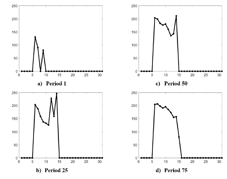
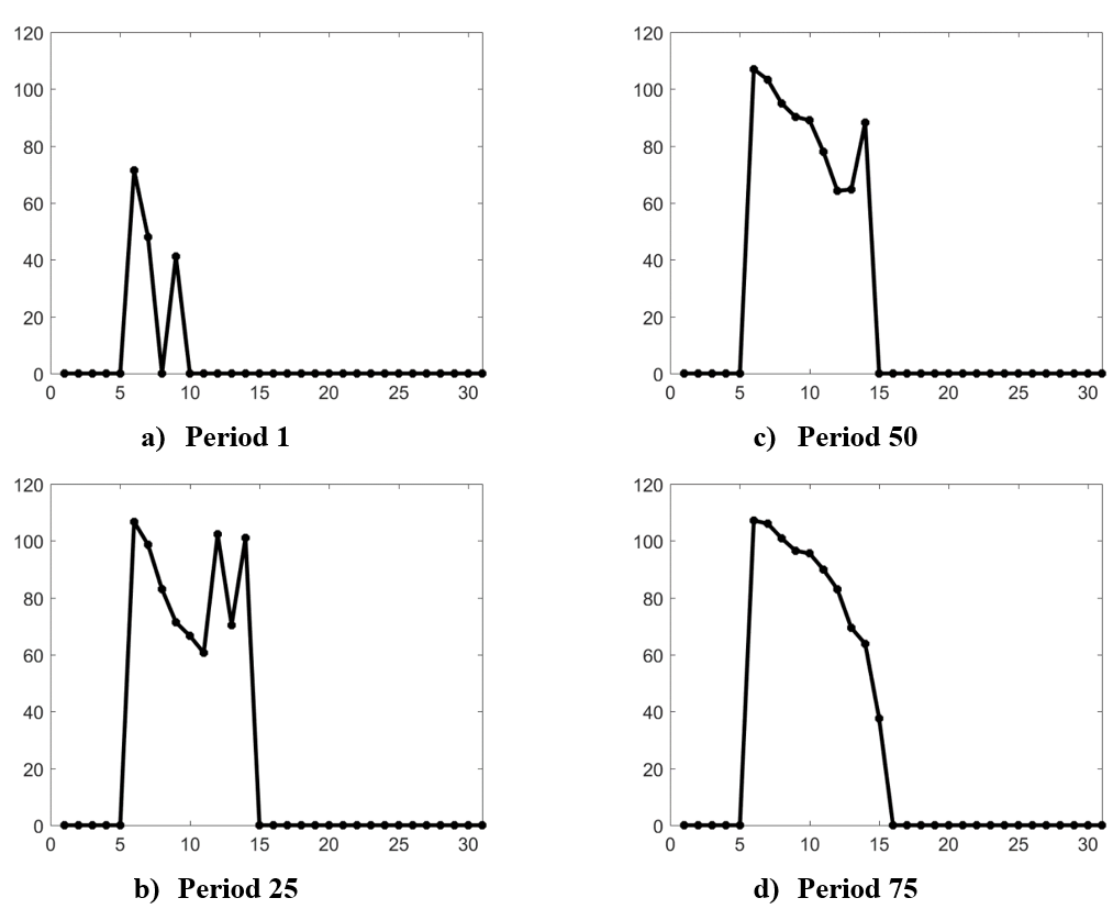
We start with baseline conditions that mimic the exurban residential land market with limited spatial competition among households. The model generates land development patterns over time along with the corresponding evolution of income and residential rent patterns. The dynamic evolutions of the income and land rent gradients from a simulation run of 100 time periods are summarized in Figures 4 and 5 respectively. Distance to the urban center is plotted on the horizontal axes and the average household income and residential rent are plotted on the vertical axes. If there is no development at a particular distance, then the average income and rent are set at zero.

In the first period, as shown in the Figures 4 a and 5 a, scattered development occurs at distance \(z=9\) because no parcel at distances \(z=8\) is developed. As time proceeds, new developments fills in the spatial gap between the scattered developments. Another interesting phenomenon is that in the early periods, some relatively rich households choose to live in more distant parcels and some not so rich households locate closer to the urban center (see Figures 4 a-b). This generates the non-downward sloping income and rent gradients in Figure 4 a-b and 5 a-b. However, income and rent gradients eventually become downward sloping as expected in equilibrium models (Figure 4 c-d and 5 c-d).

In our model, both the appearance of scattered development and the formation of downward sloping income and rent gradients are due to changes in the household spatial competition. Over time, as population grows, there are more and more households competing on the land market. This process gradually erodes the bargaining power of households and their trade surpluses from auction. This in turn, decreases the potential gains for locating in the distant parcels. When such gains are less than the increased travel cost, households will stop choosing more distant parcels. As a result, scattered development disappears and the downward sloping income and rent gradients emerges.

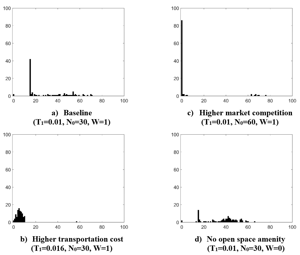
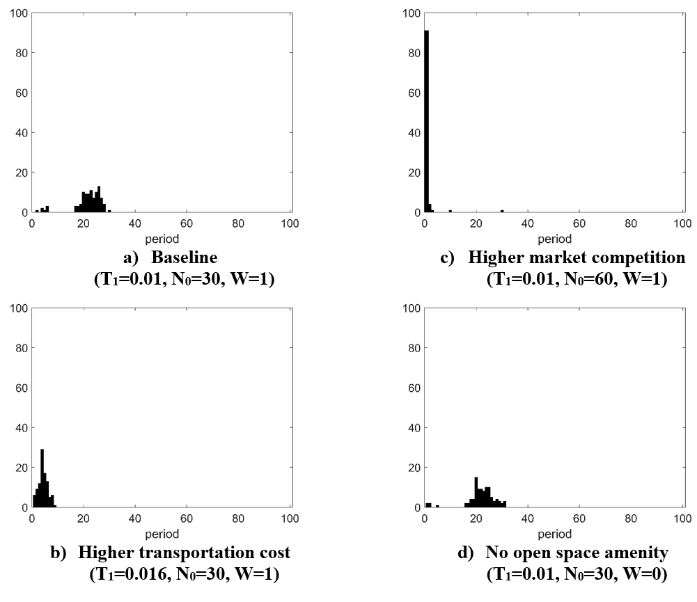
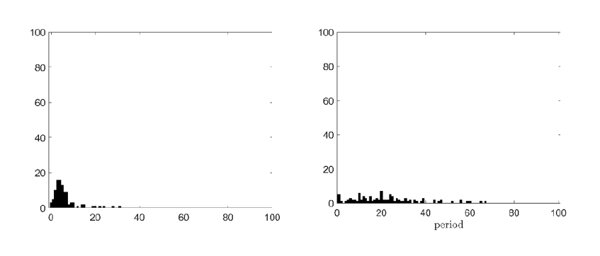
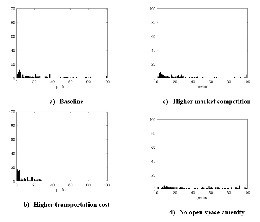
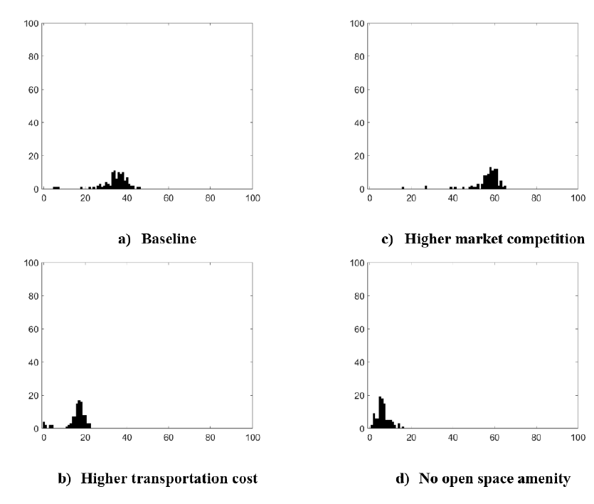
While results of one simulation are illustrative, it is insufficient for comparative static analysis due to the randomness of the model. This is particularly worrying when we try to examine the impact of key socio-economic factors on land use pattern. We therefore simulate the model 100 times for the baseline case. The histogram of the intensity measure of the scattered development is plotted in Figure 6 a, in which the x-axis plots a range of values of the intensity measure and the y-axis plots the corresponding frequency value. The histogram of the persistence measure of the scattered development is plotted in Figure 7 a.

Impacts of transportation cost

Transportation costs are considered a key factor affecting the formation of scattered development. In this paper, we illustrate how changes in transportation cost affected the formation of land use pattern through household spatial competition. Higher transportation costs imply a higher opportunity cost of living on more distant parcels. In addition, higher transportation costs reduce the parcel value (see Equation 3) as well as the potential trade surplus at more distant locations. All these factors decrease the incentive for scattered development. We therefore believe that higher transportation costs decrease the intensity and persistence of scattered development. To test this hypothesis, we increase the opportunity cost of time (\(t_{1}\)) from 0.01 to 0.016. This is equivalent to a decrease in driving speed from 50 to 30 miles per hour, or an approximately 40% increase in total transportation cost. The consequent changes in the intensity and persistence of scattered development are reported in Figure 6b and 7b. Compared to the baseline case, the histograms exhibit a significant leftward shift in both figures, indicating decreases in both the intensity and persistence of scattered development. This is consistent with hypothesis (a) in Table 2.

It is worth noting that scattered development disappears when the travel cost (time cost) is too high (\(t_{1}=0.3\)) or too low (\(t_{1}=0.001\)). If the travel cost is too high, trade surplus may not be sufficient to fully compensate for this cost. If the travel cost is too low, almost all households can afford almost any parcel, and there is no variation in market competition over the spatial extent of this study. Consequently, there is no incentive for scattered development.

Impacts of higher competition

To investigate the impact of market competition on the intensity and persistence of scattered development, we change the number of new migrants. From the individual perspective, an increase in the number of bidders implies less bargaining power for households and so, potential trade surpluses decrease. It becomes less likely that trade surpluses on more distant parcels are sufficient to cover increased transportation cost. So the probability (\(p\)) of each individual household to choose scattered development is reduced. However, from the regional perspective, the expected intensity and persistence of scattered development is given by \(N \times p\), which may increase or decrease with the increase of competing households when \(N\) is relatively small. When \(N\) is big enough, the decreases in incentive for scattered development will eventually dominate. As a consequence, the intensity and persistence of scattered development will eventually decrease with market competition. To test this hypothesis, we double the number of new migrants. In each period, we set \(N_{0} = 60\) instead of \(30\), which decrease both the intensity and persistence of scattered development, as illustrated by the leftward shifts in the histograms in Figures 6 c and 7 c.

Impacts of the preference for open space amenities

To investigate the impact of any preference for open space amenities on the land use pattern, we assume that households have no preference for open space amenities, so that the model is purely driven by income heterogeneity. To achieve this, we set the willingness to pay for open-space amenity \(w=0\). The decrease in WTP for amenities may have two counteracting effects. First, when the willingness to pay for open space amenity (\(w\)) decreases, the values of parcels with open space amenity are reduced, so are the potential surpluses (see Equation 3). Because more distant parcels typically have fewer developed parcels in their neighborhood compared to parcels close to the urban boundary, the decrease in the WTP for open space amenities has a bigger adverse impact on more distant parcels. Therefore, the decrease in trade surplus will be larger on more distant parcels. This reduces the incentive for scattered development.

Second, all other things being equal, a reduction in the WTP for parcels with open space amenities increases the minimum income \(Y_{min} (z,A)\). Because distant parcels typically have open space amenities while parcels close to urban boundary did not, a decrease in the WTP for open space amenities will disproportionately affect more distant parcels. The increase in \(Y_{min} (z,A)\) decreases the expected number of competing households \(N_{(t,z)}\) (see Equation 1). This will decrease the bid and therefore increased trade surplus. This decrease in market competition would increase the incentive for scattered development. Because the first and the second effects may act in opposite directions, it is difficult to determine which effect dominates in any given simulation and the net change could be small. This can be seen in Figure 6d and 7d.

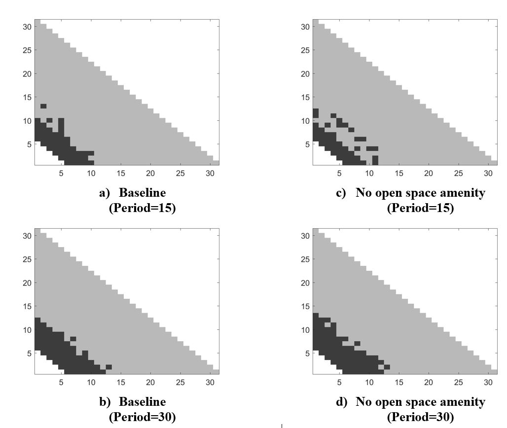
To examine the impact of open space amenity on land use pattern, the land use patterns from the baseline and those from the scenario (d) are plotted in Table 2. Figure 8 shows land use patterns in the 15th and 30th periods from each scenario. To ensure unbiased comparison, the pseudo random number generator used the same random seed for the different model specifications. Comparisons between land use patterns suggest that in this simulation, the second impact mentioned previously was dominant. The case without open space amenities generated more scattered development in this simulation. However, as indicated by the comparisons between Figures 6 and 7 a with 6 and 7d, this difference may not have been statistically significant.

Sensitivity Analyses

To investigate the sensitivity of the results, we test alternative model calibrations. We test the sensitivity to relocation. Instead of the five percent in the baseline, we set the relocation rate to be ten, twenty and one hundred percent respectively. We re-calibrate the model using data from year 2000 instead of 2010. The key conclusions of the paper are robust to these changes. Please see the results in the Appendix.

Conclusion

We develop an agent-based land market model based on Chen et al. (2017) thinly traded land market model. We modify this market model to incorporate open space amenities. In this new agent-based model of land markets, households formulate optimal bids for affordable location and landowners from their reserve price based on the opportunity cost of land and market competition. Landowners convert their land to residential development if the winning bid is greater than their reserve prices. The model incorporates several key features of exurban areas, including plentiful land supply, limited competition among households, and heterogeneous household income. By simulating this model with exogenous population growth over time, we are able to represent the evolution of land rents, income and land-use patterns in a growing urbanizing area. We find that scattered development can emerge as the result of limited competition for parcels located farther away from the urban area, but that it disappears as the region becomes more populated and competition for land increases. The simulation results show that the intensity and persistence of scattered development are systematically related to key economic factors of the model, like market competition condition, transportation costs, migration rate.

The paper makes an important methodological contribution by offering a bridge between agent-based models and the urban economics models on land use change. The bilateral negotiation, as proposed by Parker & Filatova (2008) and Filatova et al. (2009), can be regarded as the limiting case of setting the number of competing bidders equal to one on all parcels. The spatial equilibrium models in urban economics literature can be regarded as the limiting case by setting the number of competing bidders equal to infinity on all parcels.

The integration of this agent-based model with the thinly traded market theory is important for policy simulations, as it incorporates an important stylized fact in regional land market in all suburban and exurban areas. That is, land supply (demand) increases (decreases) with the distance to an urban center. These spatial differences in market competition, on both the supply and demand side, provide strong economic incentives for scattered development. More importantly, our results suggest that relatively richer households have stronger incentives for scattered development. It is interesting to explore these implications for welfare analyses, economic inequality and spatial segregation.

One limitation of this model is the assumption of constant WTP for open space amenities. In reality, this WTP may not be constant. For instance, the WTP for more durable open space amenities (like those under various conservation protections) is probably higher than less durable amenities (such as the unprotected open space under great development pressure). Future research is necessary to investigate whether these differences in the durability of open space amenities have significant impacts on the intensity and persistence of scattered development.

Another limitation of this approach is that we do not consider the possibility of multiple exurban regions. It is interesting to investigate how the increased competition for land in one exurban region may impact the development of new scattered development in other exurban areas. In addition, the model is highly stylized and omits many sources of heterogeneity that surely contribute to scattered patterns of development in reality, e.g., differences in land quality, zoning, and proximity to other urban or natural amenities. Our model simplifies the real estate and housing market by ignoring other forms of housing such as communal housing. Finally, we have not considered the durable and irreversible nature of land development in this paper. Inclusion of many of these more realistic features may reduce the amount of contiguous development and increase the intensity and persistence of scattered development, and therefore, are important questions for future research.

References

ALONSO, W. (1964). Location and Land Use. Cambridge, MA: Harvard University Press.

CAPOZZA, D., & Helsley, R. (1989). The fundamentals of land prices and urban growth. Journal of Urban Economics, 26(3), 295–306. [doi:10.1016/0094-1190(89)90003-x]

CHEN, Y. (2020). Effects of development tax on leapfrog sprawl in a thinly traded land market. Land Use Policy, 92, 104420. [doi:10.1016/j.landusepol.2019.104420]

CHEN, Y., Irwin, E., & Jayaprakash, C. (2017). Market thinness, income sorting and leapfrog development across the urban-rural gradient. Regional Science and Urban Economics, 66(3), 213–223. [doi:10.1016/j.regsciurbeco.2017.07.001]

DOU, Y., Yao, G., Herzberger, A., Silva, R. F. B. da, Song, Q., Hovis, C., Batistella, M., Moran, E., Wu, W., & Liu, J. (2020). Land-use changes in distant places: Implementation of a telecoupled agent-based model. Journal of Artificial Societies and Social Simulation, 23(1), 11: https://www.jasss.org/23/1/11.html. [doi:10.18564/jasss.4211]

ETTEMA, D. (2011). A multi-agent model of urban processes: Modeling relocation processes and price setting in housing markets. Computers, Environment, and Urban Systems, 35(1), 1–11. [doi:10.1016/j.compenvurbsys.2010.06.005]

FILATOVA, T. (2015). Empirical agent-based land market: Integrating adaptive economic behavior in urban land-use models. Computers, Environment and Urban Systems, 54, 397–413. [doi:10.1016/j.compenvurbsys.2014.06.007]

FILATOVA, T., Parker, D., & Veen, A. van der. (2009). Agent-based urban land markets: Agent’s pricing behavior, land prices and urban land use change. Journal of Artificial Societies and Social Simulation, 12(1), 3: https://www.jasss.org/12/1/3.html.

FILATOVA, T., Verburg, P. H., Parker, D., & Stannard, C. A. (2013). Spatial agent-based models for socio-ecological systems: Challenges and prospects. Environmental Modelling & Software, 45, 1–7. [doi:10.1016/j.envsoft.2013.03.017]

GROENEVELD, J., Müller, B., Buchmann, C. M., Dressler, G., Guo, C., Hase, N., & Lauf, T. (2017). Theoretical foundations of human decision-making in agent-based land use models – A review. Environmental Modelling & Software, 87, 39–48. [doi:10.1016/j.envsoft.2016.10.008]

KOCH, J., Dorning, M. A., Berkel, D. B. van, Beck, S. M., Sanchez, G. M., Shashidharan, A., & Meentemeyer, R. K. (2019). Modeling landowner interactions and development patterns at the urban fringe. Landscape and Urban Planning, 182, 101–113. [doi:10.1016/j.landurbplan.2018.09.023]

KRISHNA, V. (2010). Auction Theory. Cambridge, MA: Academic Press.

MAGLIOCCA, N., Brown, D., McConnell, V., Nassauer, J., & Westbrook, E. (2014). Effects of alternative developer decision-making models on the production of ecological subdivision designs: Experimental results from an agent-based model. Environment and Planning B: Planning and Design, 41(5), 907–927. [doi:10.1068/b130118p]

MAGLIOCCA, N., McConnell, V., & Walls, M. (2018). Integrating global sensitivity approaches to deconstruct spatial and temporal sensitivities of complex spatial agent-based models. Journal of Artificial Societies and Social Simulation, 21(1), 12: https://www.jasss.org/21/1/12.html. [doi:10.18564/jasss.3625]

MAGLIOCCA, N., Safirova, E., McConnell, V., & Walls, M. (2011). An economic agent-based model of coupled housing and land markets (CHALMS). Computers, Environment, and Urban Systems, 35(3), 183–191. [doi:10.1016/j.compenvurbsys.2011.01.002]

MANSON, S., Li, A., Clarke, K. C., Heppenstall, A., Koch, J., Krzyzanowski, B., Morgan, F., O’Sullivan, D., Runck, B. C., Shook, E., & Tesfatsion, L. (2020). Methodological issues of spatial agent-based models. Journal of Artificial Societies and Social Simulation, 23(1), 3: https://www.jasss.org/23/1/3.html. [doi:10.18564/jasss.4174]

MCCONNELL, V., & Walls, M. (2005). The value of open space: Evidence from studies of non-market benefits. Resources for the Future, Washington, DC. Available at: https://www.jstor.org/stable/resrep18160.1?seq=1#metadata_info_tab_contents. seq=1#metadata_info_tab_contents

PARKER, D., & Filatova, T. (2008). A conceptual design for a bilateral agent-based land market with heterogeneous economic agents. Computers, Environment, and Urban Systems, 32(6), 454–463. [doi:10.1016/j.compenvurbsys.2008.09.012]

ROBACK, J. (1982). Wages, rents, and the quality of life. The Journal of Political Economy, 90(6), 1257–1278. [doi:10.1086/261120]

SCHÜLZE, J., Müller, B., Groeneveld, J., & Grimm, V. (2017). Agent-based modelling of social-ecological systems: Achievements, challenges, and a way forward. Journal of Artificial Societies and Social Simulation, 20(2), 8: https://www.jasss.org/20/3/8.html. [doi:10.18564/jasss.3423]

TANG, W. W., & Yang, J. X. (2020). Agent-based land change modeling of a large watershed: Space-time locations of critical threshold. Journal of Artificial Societies and Social Simulation, 23(1), 15: https://www.jasss.org/23/1/15.html. [doi:10.18564/jasss.4226]

UNITED States Department of Agriculture (USDA). (2016). National agricultural statistics service. Available at: https://www.nass.usda.gov/Quick_Stats/index.php. Retrieved September 08, 2016.

WALLENTIN, G. (2017). Spatial simulation: A spatial perspective on individual-based ecology — A review. Ecological Modelling, 350, 30–41. [doi:10.1016/j.ecolmodel.2017.01.017]

WRENN, D., & Irwin, E. G. (2015). Time is money: An empirical examination of the effects of regulatory delay on residential subdivision development. Regional Science and Urban Economics, 51, 25–36. [doi:10.1016/j.regsciurbeco.2014.12.004]