Arguments as Drivers of Issue Polarisation in Debates Among Artificial Agents

Felix Kopecky

doi:10.18564/jasss.4767

Introduction

Two recent agent-based models of polarisation (Banisch & Olbrich 2021; Mäs & Flache 2013) rely on the exchange of arguments as a driver of polarisation. These studies underpin the hypothesis that arguments and their properties could play a role in polarisation dynamics, alongside diverse other candidate causes, such as lacking exposure to other views (Mutz 2002) or the effects of one-to-many communication in online networks (Keijzer et al. 2018).

Studying polarisation in agent-based debate models can profit our understanding of polarisation in humans in two ways. First, agent-based models can help in formulating hypotheses about which factors contribute to polarisation in humans, which then can be tested in experimental studies on human deliberation. Secondly, since agents in debate models exhibit an idealised version of rational deliberative behaviour, debate models can help us understand which extent and kinds of polarisation we will have to expect even in cases in which human behaviour approximates this kind of idealised rationality.

With the model presented in this paper, the hypothesis that arguments can drive polarisation is elucidated further: argumentation on its own can be a driver of polarisation in populations of artificial agents even when communication between agents is not governed by social influence. In models of social influence, an agent’s updating is shaped by what other agents think, in particular its close neighbours. In the model presented here, agents only listen to what the arguments say when updating, and they influence the updating of others by introducing logical constraints on which opinions they can choose.

Simulations on this model exhibit rising polarisation after argument introduction in three standard polarisation measures. But not all arguments affect polarisation equally: different strategies of selecting premises and conclusions for an argument can influence the obtained polarisation values. Two of the three measures show noteworthy differences depending on the argumentation strategies employed in premise selection. When agents take into account the opinion of a communication partner as premises (“allocentrism”), their arguments have an increased chance of facilitating low values of polarisation. Arguments that take off from premises the agents themselves hold (“egocentrism”) have a lower chance of inducing low polarisation. Additionally, when models are initialised with perfect bi-polarisation between groups, the allocentric strategies are able to de-polarise the debate towards medium levels of polarisation, while the egocentric strategies appear unable to recover from bi-polarisation.

This paper is organised into six parts. The Background Section briefly recaps the theoretical foundation of the model, reviews other agent-based debate models of polarisation and key differences to the present model, and discusses two important conceptual details of issue polarisation. The model is presented in detail in the Model Section, followed by an evaluation of experiments that track measures of issue polarisation on it (Experimental Results Section), accompanied by a robustness analysis in the Robustness Analysis Section. A Conclusion at the end summarises its results and limitations. Details about the Python implementation as well as resources to reproduce and vary the simulations are listed in the Appendices.

Background

The model presented below is based on the theory of dialectical structures (TDS, Betz 2009). In TDS, the structure of a debate is represented by a triple \(\tau = \langle T, A, U\rangle\), where \(T\) is the set of arguments, \(A\) a defeat and \(U\) a support relation on the set \(T\). Structurally, the triple \(\tau\) instantiates an abstract bipolar argumentation framework (Cayrol & Lagasquie-Schiex 2005, p. 382). Cayrol & Lagasquie-Schiex bipolar frameworks in turn are an extension of argumentation frameworks (AFs) introduced by Dung (1995). These frameworks are abstract in the sense of remaining agnostic to the internal structure of arguments and not further specifying the nature of relations between arguments. In other applications, AFs are often used to study the acceptability of arguments (for a review, see e.g. Besnard & Hunter 2008, sec. 2.2), an interest that is not pursued here. TDS instantiates these abstract frameworks by assigning meaning to the objects and relations: it characterises arguments as premise-conclusion structures and provides definitional criteria for defeat and support relations, which are explained in more detail below. TDS also introduces positions, which I use below to model agents’ belief systems, and argumentation strategies to capture intentions in argumentation.

Since AFs in general approach argumentation from a logical point of view, their representation of arguments and debates are naturally translated to Boolean formulas, and extensions such as positions are expressible in set theory. These formalisations enable the detailed study of arguments and arguers in agent-based models. This paper complements results from previous simulations on TDS debate models which have measured agreement dynamics (Betz 2013), and is based on a new software implementation for simulations on TDS models.

Review of argumentative models of polarisation

The majority of agent-based debate models do not instantiate argumentation frameworks, but there are two even more fundamental differences to the model presented here: (1) How they describe arguments and agents, and (2) which kind of argument exchange and belief updating events they implement.

Regarding the first difference, Mäs & Flache (2013, sec. 1.3.2) describe a debate as being about an issue, to which arguments provide either a reason for acceptance or refutation. This leads to a two-tiered ontology consisting of issues and arguments. The pro- and con-relations are always directed from arguments toward the issue, but never between pairs of arguments or from the issue to one of the arguments. The positions of agents are represented by numeric values that reflect their stance toward the issue, and accepting an argument changes this stance by a numeric value based on the relevance that agents assign to the argument.

Banisch & Olbrich (2021) extend the model by Mäs & Flache (2013) and account for discussions with multiple issues. In their model, arguments can be related to more than one issue (Banisch & Olbrich 2021, sec. 2.3): they may provide a reason in favour of one issue but against another one, reasons in favour of both, etc. Issues become related in this way, because an agent’s acceptance of one argument can provide it with a pro-reason for one issue and, simultaneously, with a con-reason for another issue. This model shows how the interdependence of issues can shape the positions that agents may adopt and the subsequent effects on polarisation (Banisch & Olbrich 2021, sec. 3.18).

Both models treat arguments uniformly without differences in argumentative properties. The models thus contribute to understanding the general influence of arguments on polarisation, but leave open the influence that expressions of argument properties might have. For example, they do not differentiate the diverse intentions of arguments, which are captured as argumentation strategies in the present model: these can take the form of fortifying one’s own position, of convincing others to shift towards acceptance of a conclusion, or of highlighting contradictions in the reasoning of others.

These models also limit the functions of arguments to providing reasons in favour or against an issue. Although these are clearly central functions of argumentation, not all arguments can be reduced to these roles: for example, arguments can shape debates by showing that the issues under discussion can be mutually accommodated, they can enlarge or reduce the scope of issues, etc. The effects on polarisation of these and other argumentative features are not investigated, and an argument exchange mechanism that resolves the inner workings of arguments seems necessary for this task.

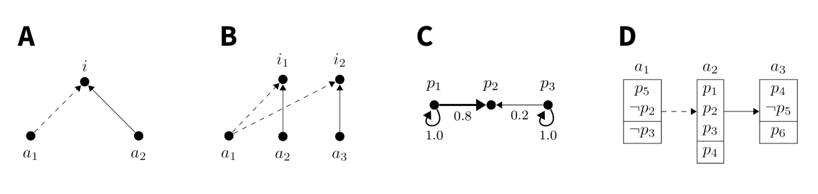
Figure 1 shows a comparison of models with respect to their conception of sentences under discussion in a debate. The models by Mäs & Flache (2013) and Banisch & Olbrich (2021) have a split ontology (with arguments and issues), and two relations that represent pro- and con-reasons, respectively. The TDS model presented here has a uniform ontology consisting of arguments only, which are further specified as consisting of premises and conclusions. In the TDS model, the defeat and support relation just mentioned replace the two relations from the first two models. The figure also shows a graph representation of propositional relations in the model by Friedkin et al. (2016).

Friedkin et al. (2016)‘s model is a general model of opinion dynamics and not a specific model of polarisation. It is interesting when studying TDS models though, because both encode logical constraints in opinion dynamics: Friedkin et al. (2016) use a matrix \(C\) with elements \(c_{ij} \in [0,1]\) showing the logical constraint of sentence \(i\) on sentence \(j\), while the model presented here uses Boolean formulas to store logical constraints. In Friedkin et al.’s model, the effects from the logical constraints in the matrix \(C\) compete with influences from a social network in forming agents’ belief systems. The matrix \(C\) is stochastic, which requires that the row sums equal 1. In the graph representation, this translates to all constraints on a proposition adding up to 1 in their weight, including reflexive constraints.

Another example (not pictured in Figure 1) for combining the effects of logical constraints and social networks is the model by Butler et al. (2019). In fact, this model also uses argumentation frameworks, but in comparison to the present model, theirs is built on argumentation frameworks in the original sense (Dung 1995), which means that arguments can only stand in defeating relations toward other arguments and are not resolved further in terms of premises and conclusions. A further difference is that agents are directly affected by the opinions of others in their model, and that this impact depends on the antecedent opinion difference.

**Figure 1.** Illustration of selected models and their representations of the sentences under discussion, interpreted as directed graphs. (A) and (B) show Mäs & Flache (2013)’s and Banisch & Olbrich (2021)’s models, respectively. Those two distinguish issues \(i_j\) and arguments \(a_k\). Dashed edges show arguments supporting a negative stance toward the issue (contra arguments), and solid edges support a positive stance (pro arguments). In (B), more than one issue is considered in a debate, and not every argument needs to contribute to every issue. (C) illustrates Friedkin et al. (2016)’s model, in which nodes represent propositions and edges show the weight of doxastic implication: in this example, an agent’s belief in \(p_1\) implies belief in \(p_2\) to a degree of 0.8, and an agent’s disbelief in \(p_1\) would imply disbelief to the same weight, but its belief in \(p_1\) is not constrained by belief in another proposition. An example for debates in the TDS model from this paper is in (D), where nodes are arguments consisting of premises and conclusions, and edges are either of the support or defeat relation.

A second important difference between agent-based debate models is how they have agents behave toward each other and how agents update their belief systems. Mäs & Flache’s and Banisch & Olbrich’s are social influence models (SIM, see Flache et al. 2017 for a typology). In SIM, the opinions that agents move to in an updating event are aggregates of the distances between the updating agent and the agents that influence it. For example, in assimilative SIM, the opinion of an agent at time \(t+1\) is given as the agent’s position at \(t\) plus the sum of weighted distances to all other agents in the agent’s network, normalised by an influence parameter. In contrast to this updating mechanism, agents in the model presented below are only indirectly influenced by the belief systems of other agents, through the arguments those agents introduce. Agents decide how to change their opinion based on maximal opinion continuity, and do not rely on particular neighbours for their updating.

The updating process in models of source reliability (Merdes et al. 2020) is reminiscent to that in SIM, and some of these aim to model polarisation in debates (Olsson 2013; Pallavicini et al. 2021). An important difference to SIM is their usage of conditional probabilities in the updating processes: agents are influenced by their communication partner according to a probability conditional to the agent’s trust into its partner (Bayesian updating). Note that trust need not be identical to similarity in SIM (agents can trust others even if they are far removed). But the ultimate driver of polarisation in these Bayesian models can not be seen to be argumentative, since trust in other agents is an epistemic property of the agents, not one of the produced arguments.

The model presented below does not only differ in how agent’s belief systems are influenced by others, but also which agents can exert this influence. Mäs & Flache’s and Banisch & Olbrich’s models only yield polarised outcomes when they rely on homophily to determine which agents are partnered up in an argument exchange event (see Figure 7 in Banisch & Olbrich (2021) and Figure 3 in Mäs & Flache (2013) for the effects of homophily in their models). In the context of these models, homophily basically means that agents are more likely to communicate the more alike they are. While this influence is a well-established phenomenon in the communication of humans and an interesting factor in its own right (McPherson et al. 2001), its influence may limit the insights to be gathered about arguments as drivers of polarisation. Homophily, after all, is not a property of arguments, but of the agents. The model presented here is different in that respect: it exhibits rising polarisation even as all agents communicate in a continuous debate forum, with all of them having equal probability to select each other as communication partners.

Details on the concept of polarisation

Issue polarisation is the target phenomenon of the model below, and although it is intuitively easy to understand, it is also a theoretical concept that has recently seen substantial conceptual and empirical contributions. The distinction between issue polarisation and (dis-)agreement is also interesting, since both are properties of a populations’ opinion distribution. The next two sections briefly review differences between (1) social and issue polarisation and (2) measuring issue polarisation and measuring agreement.

There are at least two types of polarisation

There are a number of ways to understand polarisation (Iyengar et al. 2012, 2019; Mason 2013), and a model that concentrates on the arguments in a debate is particularly designed to track polarisation in reasons and opinions, which is known as issue or belief polarisation. Such a model has a harder time to track other aspects of polarisation, particularly social polarisation (also called behavioural polarisation with the important sub-type of affective polarisation). Put broadly, social polarisation is a state of affairs in which members of a population cease to view other members as enrichment, partners in collaborative projects, etc., and begin to see them primarily as a likely source of harm (either toward themselves or toward others one cares about), a threat to the well-being of society, etc.

For the US public, the Pew Research Center (2014) extensively studies effects of both types of polarisation. The United States are occasionally cited as an example of a polarised society, but this picture needs specification. Summarising research on her own country, Mason (2015, pp. 131–132) finds that effects of social polarisation are more pronounced than those of issue polarisation, leading her to conclude (2015, p. 142) that “the outcome is a nation that may agree on many things, but is bitterly divided nonetheless”.

For the interpretation of polarised outcomes in agent-based models, this constitutes an important caveat: it is important to distinguish issue from social polarisation in these models, because polarisation in terms of on-topic opinions can develop independently of how disputants regard other parties in the discussion. Results obtained on one type should not be applied to understanding polarisation in general, which is particularly true for the model presented below.

Polarisation as a concept gets even trickier since its two sub-types differ in scope. Issue polarisation is not restricted to debates in politics, but can be expected in other deliberative populations as well, such as scientific communities or in the courtroom. It is a property of particular debates (on particular issues with particular agents), compared to social polarisation, which is a property of populations as a whole and has so far been reported in the general public and in politically engaged groups, but its role in specialised communities is unclear and possibly lower. An important question then arises about the correlation between these two kinds of polarisation. While Mason (2015) is clear that social polarisation does not seem to correlate with the mean issue polarisation across a range of issues, it may still turn out that social polarisation does correlate with specific issues polarising.

Measuring polarisation is different from measuring (dis)agreement

If issue polarisation is characterised by divergence in on-topic views, a good question to ask is how this fits into the overall study of debates and deliberation. In particular, how does studying polarisation differ from studying disagreement?

Betz (2013) measures disagreement in a population of agents as the averaged normalised distance between pairs of agents’ belief systems, and agreement as the inverse of this value. Let \(\delta\) be a distance measure between two agents, such as the Hamming distance of their belief systems, \(n\) the number of sentences under discussion and \(A\) the population of agents. Then the population-wide mean agreement (PWMA) is given as:

\[\text{PWMA}(A) := \frac{1}{\left|{A\choose 2}\right|} \sum_{(x,y) \in {A\choose 2}} 1-\frac{\delta(x,y)}{n}\]

\[(1)\]

In PWMA, the inverse of normalised differences (\(1-\delta(x,y)/n\)) is averaged over the pairs of agents in the population, but no further aggregation of the atomic \(\delta\)-values takes place, which means that differences contribute uniformly to the measure. This is different to polarisation measures, which aggregate the same normalised difference values: they either track how these measurements spread around the mean difference, or aggregate the differences based on group membership of the individual agents. Measuring polarisation thus goes beyond reporting an absence of agreement in a population and further characterises such disagreement in terms of variation and clustering.

The Model

This section presents the model according to Grimm et al. (2006)'s ODD protocol.

Overview

Purpose

This model is designed to study the effects of argument introductions and argumentation strategies on issue polarisation in debates among artificial agents.

State variables and scales

Debates in this model are simulated as the logical conjunction of arguments. Arguments are logical implication relations between a set of premises and a conclusion. Both premises and conclusions are drawn from a sentence pool, which consists of \(n\) atomic sentence variables and their negations, meaning it has \(2n\) elements. Every argument introduced to the debate must meet these criteria:

Satisfiability: A debate must remain satisfiable at all times. That is, the conjunction of arguments must be satisfiable.
Premise uniqueness: Every argument must have a unique set of premises, i.e., any set of premises can be used in at most one argument of the debate. This restriction does not hold for conclusions, i.e., can be multiple arguments with the same conclusion.
Prohibition of conflicts and redundancy: If a sentence is used as a premise, neither it nor its negation is used as the conclusion or another premise of the same argument.

A debate is represented by a Boolean expression of the conjunctive form in (2).

\[ \underbrace{((p_a \land ... \land p_b) \implies p_c)}_{\text{Argument 1}} \quad\land\quad \underbrace{((p_d \land ... \land p_e) \implies p_f)}_{\text{Argument 2}} \quad\land\quad ...\]

\[(2)\]

The arguments and the debate as a whole use sentence variables, and the model is thus abstracting from the actual propositional content of premises and conclusions. This is sufficient for the purpose of investigating the general role of argumentation in polarisation dynamics, but building debates on sentence variables can not elucidate the role of particular propositional contents in premises (such as the difference between normative and descriptive claims) or of actual argumentation schemes. Natural language argumentation technologies seem necessary for this task, and it will be interesting to see how emerging approaches to natural language processing of argumentation (Betz 2021; Hunter et al. 2019) can be employed in future research.

Agents in this model are simulated as having a belief system represented by positions in terms of TDS, and I will use both terms interchangeably in this paper. Positions are mappings from the atomic sentence variables to truth values True and False. An agent’s belief system is fully specified by these truth-value attributions. In this model, agents assign a truth value to every sentence in the sentence pool (they never suspend judgement), but are confined to satisfying interpretations of the debate, which means that every agent must hold a position that is an interpretation of the Boolean formula that describes the debate. This minimal picture of rationality implies that agents assign identical truth values to equivalent sentences but different truth values to contradictory sentences, and follow their inferential obligations: if an agent assigns True to all premises in an argument, it also assigns True to the conclusion.

For a simulation with \(n\) sentence variables in the sentence pool, an agent’s position can be represented as in (3):

\[\begin{equation} \begin{split} p_1 \to & \; True\\ p_2 \to & \; False\\ & {\vdots}\\ p_n \to & \; \; \ldots \end{split} \end{equation}\]

\[(3)\]

Agents that assign True to an atomic sentence variable are said to “accept” it, otherwise they “reject” it. Besides a so-defined belief system, agents are associated with one of the five argumentation strategies (described as part of the argument introduction sub-process below). In every model run, all agents share the same argumentation strategy. Distances between positions of any two agents are measured by means of the Hamming distance, which is interpreted to be the number of sentences that are mapped to a different truth value.

A debate stage is described by the debate at that time (the current state of the conjunction of the arguments) together with the agents’ current positions. There are a number of high-level properties that can be obtained from these lower-level properties. The first object of interest here is the argument graph. An argument graph is a two-coloured directed graph that takes the arguments in the debate as nodes and defeat and support relations as edges. A pair of arguments \((a,b)\) satisfies the support relation if the conclusion of \(a\) is equivalent to one of the premises in \(b\), and the pair fulfils the defeat relation if the conclusion of \(a\) is equivalent to the negation of one of the premises in \(b\). This means that the relations between arguments are automatically obtained from the arguments. Argument graphs are not necessarily complete, and are non-circular more often than circular. The argument graph of a debate stage \(i\) is referred to as \(\tau_i\).

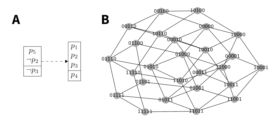
A second group of higher-order properties of a given debate stage concern its space of complete and coherent positions, represented as \(\Gamma_\tau\) (SCCP, Betz 2013, pp. 39–41). In logical terms, the SCCP is the set of all satisfying interpretations of the Boolean formula that represents the debate at a given stage (see Figure 2 for an example). It should be noted that the SCCP is very different to, and usually contains much more elements than, the collection of actually held positions by the simulated agents. Actually held positions have to be in the SCCP, but multiple agents can hold the same position from the SCCP, and the actually maintained positions in the simulation can be quite spread out in the SCCP. In terms of the model, the SCCP is the set of positions that the actual agents are allowed to move to should their positions be rendered incoherent by the introduction of an argument. A position is incoherent relative to a debate stage if its assertions are jointly unsatisfiable with the arguments at that debate stage. Other than that, the model allows agents to move freely in the SCCP. In particular, it does not prescribe them to favour positions with maximal quantitative argument support, or to move toward positions held by other agents. This seems realistic considering that it can be rational to adopt a position even if there is just a single argument in its favour, namely when the single argument is especially convincing. Argument evaluation and a measure of argumentative strength are not part of this model, however.

**Figure 2.** (A) Argument graph for the debate stage \(((p_1 \land p_2 \land p_3) \implies p_4) \; \land \; ((p_5\land \neg p_2) \implies \neg p_3)\), and (B) the resulting space of coherent and complete positions (SCCP). In the argument display, premises and conclusions are separated by a horizontal bar, and the defeat relation is expressed with a dashed arrow. In the SCCP, nodes have a label that shows the bit string representation of the position they resemble. In this string, sentences are ordered alphabetically (\(p_1\) will show in the first bit, \(p_5\) in the last), and they are either 0 if the position assigns False to this proposition, or 1 if the position accepts the proposition. Positions are connected by an edge if they differ in exactly one truth-value attribution (i.e., if their Hamming distance equals 1).

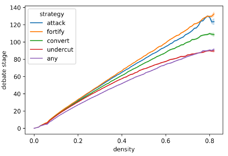
The size of the SCCP, \(|\Gamma_\tau|\), is used in calculating a debate stage’s density, a fundamental measure of progress in debate simulations (Betz 2013, pp. 44–49). Roughly speaking, density encodes how many positions have been rendered incoherent so far in the debate, and how much freedom the agents have in choosing the next position to move to if they have to. Importantly, not every argument introduction raises the debate’s density in the same way, and debates can take up to twice as much argument introductions to reach the same density. A debate stage’s density is always in the \([0,1]\) interval, and defined as \((n-\log_2 (|\Gamma_\tau|))/n\), where \(n\) is the number of atomic sentence variables (Betz 2013, p. 44). Figure 12 in Appendix B shows how density evolves over simulation time depending on the different argumentation strategies.

The most important parameters of the model and initial settings for the main experiment are described in Table 1. Almost all of them influence the simulation’s computation time. The number of premises per argument is initially chosen as the range 2–3, but a robustness analysis was run on 2–4 sentences per argument. This parameter can be either a number or a range. If it is a range, the number of premises in any introduced argument is chosen randomly. The number of atomic sentence variables and the termination density are taken as best practices from Betz (2013). The number of agents are chosen somewhat arbitrarily, but robustness analyses are provided for smaller populations and sentence pools (which actually confirm and exceed the results). Varying the size of the sentence pool does exponentially influence the run time of experiments. Given the current software implementation and the available computational resources for conducting the experiments reported below, a size of 20 atomic sentence variables, resulting in a sentence pool of 40 sentences, proved workable.

**Table 1:** Description of the model parameters and values adopted in the main experiment
Parameter	Value
No. agents	50
No. atomic sentence var.	20
No. premises per argument	2 or 3
Argumentation strategy	Either of five
Updating strategy	Closest coherent
Initial positions	Random
Max. density	0.8

Processes and scheduling

The simulation proceeds by two kinds of events: argument introduction and a following position updating, and simulation time is understood as numbers of introduced arguments. At every step, both events are called until limiting conditions are met. The model terminates either when a density greater or equal than the maximum density parameter is reached, or if an argument introduction fails due to lack of premises or conclusions meeting the requirements imposed by the strategy.

For each argument introduction, two agents are randomly drawn from the population. The first agent is understood to be the source, the second one is called target. The source then acts according to its associated argumentation strategy. A single model run assigns the same strategy to all agents, which can either be one of the four basic ones (Betz 2013, pp. 93–94):

Attack: From the sentence pool, the source picks premises that it accepts and a conclusion that the target rejects to build a valid argument. The source also ensures that the conclusion does not contradict its position.
Fortify: From the sentence pool, the source position selects both premises and a conclusion that it accepts to construct a valid argument.
Convert: From the sentence pool, the source position selects premises that the target accepts and a conclusion that the source accepts to build a valid argument.
Undercut: From the sentence pool, the source position picks premises that the target accepts and a conclusion that the target does not accept to construct a valid argument. The source also ensures that the conclusion does not contradict its position.

Agents can also have a fifth strategy, which picks a strategy at random for each argument introduction:

Any: The source randomly chooses one of the four basic argumentation strategies to introduce a valid argument.

When this argumentation process is completed, all agents in the population check whether their positions are rendered incoherent by the new argument. From the logical point of view, an interpretation can satisfy one Boolean formula, but not the updated conjunction of the Boolean formula and an added formula (i.e., the previous debate extended by a newly introduced argument). When this happens, a position is rendered incoherent. In the model, all the agents with incoherent positions following argument introduction immediately update their position. Figure 11 in Appendix B shows how many agents, on average in the model runs of the main experiment, update their position following argument introduction. As can be seen, the undercut strategy has the agents update considerably more often than the other strategies. As the SCCP shrinks and density rises accordingly, there is comparatively high pressure on the agents to update their positions. After all, a shrinking SCCP implies that a decreasing number of positions are acceptable to the agents.

The position update strategy that all agents share points them to their respective closest coherent position from the SCCP. “Closest” is understood to mean lowest Hamming distance. When there are several coherent positions with minimal Hamming distance, one of them is chosen randomly. Distances to the positions held by other simulated agents do not influence the updating process.

Design concepts

After this technical review of key objects and processes, let me provide a more conceptual reflection of the model’s properties.

Emergence: The starting positions of agents are randomly assigned at the start of each model run. However, agents autonomously select their subsequent updated positions based on coherence criteria. Levels of polarisation in this sense emerge from the model.
This is also true for the relation between propositions: whether an agent can simultaneously accept two items from the sentence pool depends on the autonomously introduced arguments.
Adaptation: Agents update their position if a newly introduced argument renders their position incoherent. They do so by moving to the closest neighbour among the remaining coherent positions in the SCCP, or selecting a random next neighbour if more than one have minimum Hamming distance to their previous position. In this way, only the logical relations matter for an agent’s adaptation.
Although more than one agent can hold a coherent position, agents select the closest position among all coherent positions, not just those that are currently held by other agents in the simulation. If updating is required, they choose one of the coherently adoptable positions without regard for what others believe, even their closest neighbours.
Fitness: Agents have only two goals. The first is upholding a coherent position, which they maintain by the adaptation process just described. Their second goal is to introduce arguments according to their assigned argument strategy if the model determines that it is their turn. Agents always fulfil both goals: since there is no distance limit in selecting a new position, updating always succeeds for every agent. Also, the simulation stops when one agent is unable to introduce an argument according to its argumentation strategy. Polarisation is thus not introduced due to agents’ inability to accomplish their goals.
Sensing: Agents that are selected for argument introduction know their own position and the one of the other agent in the turn. They are aware of the complete sentence and premise pool.
After argument introduction, all agents recognise whether they need to update their position or not. Those that do are aware of all of their options, i.e.know all the remaining coherent positions in the SCCP and their own position’s distance to them.
Interaction: Agents interact in terms of argument introduction described above. Agents are indirectly influenced by the actions of other agents when their position is rendered incoherent and they are forced to update.
The interaction of agents is affected only by random processes. For example, agents do not prefer to introduce attack arguments against agents with a high Hamming distance to their position. They are also ignorant to what relations their introduced argument will have to existing arguments.
Agents impact the opinion dynamics of others by introducing logical constraints to the debate. For a minimal example, consider two agents with positions \(a_1 = \{p_1 \to \text{True}, p_2 \to \text{True}, p_3 \to \text{False}\}\) and \(a_2 = \{p_1 \to \text{False}, p_2 \to \text{False}, p_3 \to \text{True}\}\), and consider that \(a_1\) would introduce the valid argument \((p_1 \land p_2) \implies \neg p_3\), thus reflecting its truth-value attributions. The argument stands against \(a_2\)’s belief in \(p_3\), but is \(a_2\) forced to update its system of belief because of the argument? No. \(a_2\) does not accept \(p_1\) and \(p_2\), and so does not need be moved by an argument that relies on their truth. If \(a_2\) would accept both \(p_1\) and \(p_2\), then giving up \(p_3\) would result in the shift to the closest coherent position.
This simple example illustrates how agents only have intermediate control over the beliefs of others. Through their argument introductions, agents shape the space of complete and coherent positions. But what the other agents make of their options is a different issue.
Collectives: Agents are not grouped into collectives. The population is regarded as a uniform whole.
Observation: Among others, the model tracks every agent and its position at every debate stage and the density of that stage. These are the two fundamental variables for calculating polarisation measures. The current implementation of the model logs more information about the model run, including position updating at each stage, and all of the arguments introduced at any given debate stage.

Details

Initialisation

At the start of every simulation, the sentence pool is generated. In the main simulation presented below, the sentence pool is generated from 20 atomic sentence variables, \(p_1, p_2, ..., p_{20}\), and their negations, \(\neg p_1, \neg p_2, ..., \neg p_{20}\). The sentence pool thus consists of 40 sentences. From this pool, a premise pool is constructed. The premise pool consists of all combinations of sentences that can be used in an argument. Given that the argument length is set to 2 or 3 premises and given the condition that an atomic sentence variable should appear only once in the premises of each argument, the number of possible combinations of premises is 9880:

\[{40\choose 2} - 20 + {40\choose 3} - 20\cdot 38 = 760 + 9120 = 9880\]

\[(4)\]

Agents select their initial position by randomly assigning truth values to every atomic sentence variable (though see Robustness Analysis Section which varies this initial setting). In the simulations below, these truth values are either True or False, and simulating positions with probabilistic assignments is left for future research. The debate contains no arguments at the beginning of the simulation.

What kind of debates are simulated with the initial values for the main experiment? With 50 participants and 40 sentences under discussion, these artificial debates could model political deliberation in parliament or scientific deliberation at a conference (think of a panel and its audience), or of the participants at a citizen deliberation event. However, the fact that there is a continuous debate forum and no side conversations take place is a simplification over the real-world originals, while the restriction of arguments with 2 and 3 premises is due to computational limitations.

Input

Input to the model is limited to the settings in the model initialisation. Environment variables such as the premise pool and the space of coherent and complete positions change only based on the agents’ behaviour, as described in the two sub-modules.

Sub-modules

There are two noteworthy sub-processes that shape the evolution of debates in the model. Both have elements of random choice – which is why the model should be evaluated in simulation experiments with many runs.

Argument introduction: At every debate stage, two agents from the population are drawn at random. Depending on the argumentation strategy, the first agent (the source) then draws premises from the premise pool that meet the criteria imposed by the strategy. For example, in the convert strategy it will draw a random set of premises that is accepted by the target agent. The fortify strategy is a special case in this regard, since it does not require inspecting the target’s belief system.
Next, the source agent looks for a conclusion from the sentence pool that (a) is not equivalent or contradictory to one of the premises and (b) meets the criteria that the argumentation strategy imposes on conclusion choice. For example, in the convert strategy, this conclusion must be one that is currently accepted by the source agent. The search continues until a valid argument is found, i.e.that is jointly satisfiable in conjunction with the arguments already present in the debate. When the introduction succeeds in this manner, the set of selected premises is removed from the premise pool, which means that this set of premises is unavailable for subsequent argument introductions for the rest of the model run. If no valid argument can be found for this particular pair of agents, the process is repeated at most \(A/2\) times by drawing another pair of agents from the population, where \(A\) is the size of the population.
It should be noted that argument introduction almost always changes the extension of the space of coherent and complete positions, although argument introductions can differ significantly in their impact. Argument introductions can render previous positions incoherent, and are the driver behind agents updating their positions in the course of the debate.
Position updating: Newly introduced arguments can render existing positions incoherent, and they regularly do. After each argument introduction, all agents in the debate check whether their position is still valid given the new debate stage, and all agents that now hold incoherent positions update them.
For all agents, the update strategy in this model is always the move to the closest coherent position. In order to find the closest coherent, every agent with an incoherent position compares its position to all coherent positions in the SCCP, and moves to the one with minimal Hamming distance. If there are multiple positions with minimum distance, one is chosen at random.

Experimental Results

Experimental design

Since argument introduction and position updating include elements of random choice, it is unavoidable to study the model in simulation experiments with many iterations. In this section, I present the results of seven experimental settings. The main experiment has a population of 50 agents and 20 atomic sentence variables, resulting in a sentence pool of 40 sentences. In a robustness analysis, I also study the model in conditions of (1) 20 agents and 20 sentence variables, (2) 20 agents and 10 sentence variables, (3) 10 agents and 5 sentence variables (resulting in a sentence pool of 10 sentences), (4) 50 agents and 20 sentence variables, but an argument length of 2–4 premises instead of 2–3, (5) with initial positions in perfect bi-polarisation and (6) with a clustering on a subset of key issues. This robustness analysis does not only confirm the results from the main experiment, but shows that polarisation effects can be amplified by contraction of the population and in particular the sentence pool.

There are a total of 5,000 experiments in each setting, 1,000 for each argumentation strategy. Apart from varying population size, sentence pool, and, in one case, length of arguments, all experiments have the same set-up: all five argumentation strategies are compared in each experiment and the experiment always runs until either a density of \(\geq0.8\) is reached or an argument introduction fails, whichever occurs first. In the main experiment, all debates end due to the density condition. Termination there occurs on average after 110 turns for convert model runs, 91 in undercut, 131 in fortify, attack models take 126 on average, and models with the any strategy 92. All in all, the data for the main experiment consist of 548,958 debate stages. I evaluate the model runs by applying three polarisation measures, all of which are adapted from the definitions in Bramson et al. (2016): dispersion, group divergence and group consensus. All measures return values in the \([0,1]\) range.

The observed values for issue polarisation are lower in this model than in other studies, and only a low percentage of simulations end in clear-cut bi-polarisation (which happens frequently in the social influence and Bayesian models discussed above). But it is important to keep in mind that this model only accounts for the influence of arguments and argumentation strategies on polarisation, and drivers such as homophily as well as other properties of agents are ignored.

Dispersion, understood as standard deviation

Dispersion tracks an intuitive idea of how agents and their belief systems can polarise by measuring how agents deviate from a population-wide mean. If these spread out evenly or cluster around one pole, dispersion will be low, but clustering around an increasing number of poles will lead to increased dispersion.

When agents’ belief systems are understood in terms of positions toward a debate stage, it is usually impossible to define a population-wide mean. This is because there will often be several, but distant, positions that likewise maximise centrality measures, and graphs on positions often have more than one graph centre.

A way to avoid this is to replace the mean position with the mean distance between all pairs of positions, and then inspect the dispersion of distances around that mean. But one must be careful here to select a polarisation measure that is an aggregation of distances – merely interpreting the average distance between pairs of agents as dispersion would lead to a concept of polarisation that is too close to a concept of agreement. Following Bramson et al. (2016, p. 84), I use the standard deviation of pairwise distances as a measure of dispersion (Definition 1).

Definition 1. Dispersion, understood as the standard deviation on the pairwise distances between agents’ belief systems. Let \(\delta\) be the Hamming distance and \(A_\tau\) the set of agents at debate stage \(\tau\), represented by their positions. \(\smash{A_\tau\choose 2}\) denotes the pairs of agents in the population. With \(N=|A_\tau|\), dispersion is defined as:

\[\text{dispersion}(\tau) := \Bigg(\frac{1}{N}\sum_{i\in A_\tau}^{N}\Bigg(\frac{1}{N-1}\sum_{j\neq i}^{N-1} \delta(i,j) - \underbrace{\frac{1}{\left|{A_\tau\choose 2}\right|} \sum_{(x,y)\in{A_\tau}} \delta(x,y)}_{\text{mean distance (constant)}} \Bigg)^2\,\Bigg)^{1/2}\]

\[(5)\]

Note: This is an instance of the common SD measure from statistics. \((...)^{1/2}\) is used here instead of \(\sqrt{(...)}\) for cleaner display.

Figure 3 shows the development of dispersion depending on argumentation strategy and plotted against density in the main experiment. It allows for a very general inspection of polarisation, and shows that the introduction of arguments generally increases polarisation. The argumentation strategies differ in their contribution to polarisation, which is comparatively high in the attack and comparatively low in the convert strategy. Agents with the any strategy show a slightly higher rate of polarisation in lower density, but end up less polarised than the attack and fortify model runs. This seems to indicate that the different effects of the strategies seem to balance each other out when triggered in alternation.

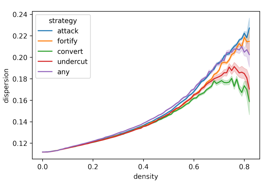
**Figure 3.** Mean dispersion plotted against density and depending on argumentation strategy in the main experiment. Shaded areas show confidence intervals based on statistical bootstrapping.

When simulations reach densities of around 0.8, the model runs are about to terminate after each agent has introduced 1–2 arguments on average, and the effects of argumentation will be most visible in this period. At densities of around 0.8, the mean values for attack simulation runs are higher than in other strategies, particularly for convert and undercut (see Figure 13 in Appendix C). The latter more often reach lower dispersion values than the other strategies, and some of the simulation runs have dispersion values comparable to their initial values, going against the general tendency.

Group-based measures

Dispersion measures pairs of agents uniformly and is ignorant as to whether they are members of different communities, or groups. Group-based measures (as defined by Bramson et al. 2016, pp. 89–93) rely on the community structure, or clustering, of the population and treat distances between neighbours (members of the same group) different to strangers (members of different groups). Groups can be determined either endogenously or exogenously (Bramson et al. 2016, pp. 87–88). An endogenous definition works on the structure of the population alone, such as in community structuring algorithms. Exogenous definitions require the addition of pre-defined criteria to partition the population into groups.

While the model could be adapted to structure its communities exogenously (for example, by adding a central thesis or background beliefs to the debate and forming groups based on whether agents accept them), in its current form the model recommends an endogenous approach. For this, I have utilised two state-of-the-art clustering algorithms: Leiden (Traag et al. 2019), a modularity maximisation algorithm, in the implementation from python-igraph version 0.9.1 (Csárdi & Nepusz 2006), and affinity propagation (Frey & Dueck 2007) from scikit-learn version 0.24.1 (Pedregosa et al. 2011). The results below are mostly reported following the Leiden clusterings, while affinity propagation was used to compare and legitimise the Leiden clusterings.

The input to each clustering algorithm is the distance matrix of the population of agents, where the values are the Hamming distance between the agents’ positions, normalised by the number of sentences (i.e., \(\text{HD}(x,y)/40\) for agents \(x,y\) in the main experiment). For Leiden and affinity propagation, these distances were transformed by \(\exp(-4x)\), and resulting values below 0.2 filtered out. This reduces the numbers of edges in the graph, which improves the clustering for Leiden. Leiden seems to expect sparsely connected graphs (as common in social networks), and the transformed and filtered distance matrices lead to a success rate consistently above 90%. Transformation and filtering also improve the convergence rate for affinity propagation, which then is around 80–90%. Both algorithms output non-overlapping clusters and are deterministic, i.e.output the same clustering for the same input every time they are run.

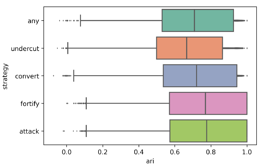
Since there are no previous reports of applying Leiden and affinity propagation to agent-based debate models built on TDS, it is important to ensure that these algorithms return reliable results. One way to measure the quality of clusterings is the adjusted Rand index (ARI, Hubert & Arabie 1985). The ARI compares two clusterings by looking into how many agents are clustered into the same group in both clusterings, and how many are clustered into different groups. For the present purpose, I apply the ARI to count how many pairs of agents that are clustered into the same community in one debate stage are also members of the same community in the following debate stage, thus measuring in how far an argument introduction changes the clustering. A low ARI indicates that many agents have been clustered differently compared to the previous debate stage, while a higher ARI shows that more agents are in the same cluster as before, thus implying a lower mobility of agents and less force of arguments to influence the composition of groups. Then, the goal is to have a somewhat high, but not too high mean ARI value that can confirm the intuitively plausible expectation that the majority of agents remain in their group in most debate stages. The model should also allow for some fluctuation in the ARI, because some argument introductions have little if any effect on the debate, while others convince many to change their views. In the evaluation of the model, the ARI between pairs of adjacent debate stages took a median value of about 0.7, depending on the argumentation strategy (see Figure 10 in Appendix B). The observed values indicate that clusterings based on the model are stable enough to simulate intuitively plausible opinion dynamics, and are thus reliable.

Group divergence

An interesting question to ask about a population’s community structure is how far apart its groups are, or what their degree of divergence is. In Bramson et al.’s understanding, this measure compares the group opinion means (2016, p. 91). As before, since the concept of a mean is hard to apply if belief systems are modelled as positions toward debate stages, I use the averaged distance value between all position pairs instead of a single value for the group.

In divergence, this translates into how, for each agent, the distances to neighbours deviate from the distances to its strangers. This then gives a measure of how distant the groups are. See Definition 2 for my formulation.

Definition 2. Group divergence, based on Bramson et al. (2016, pp. 90–91). As before, let \(A_\tau\) be the population of agents at debate stage \(\tau\), represented by their positions. Let \(\delta\) be the Hamming distance. For a position \(x_i\), \(G(x_i)\) is the set of positions of the same group (neighbours), while \(\neg G(x_i)\) are the out-group positions (strangers) determined by the algorithm. Note that \(|\cdot|\) denotes either the cardinality of a set or the absolute value of a distance, depending on its argument.

\[\text{divergence}(\tau) := \frac{1}{|A_\tau|} \sum_i^{|A_\tau|} \left| \frac{ \sum_{j \in G(x_i)} \delta (x_i, x_j)}{|G(x_i)|} - \frac{ \sum_{k \in\neg G(x_i)} \delta (x_i, x_k)}{|\neg G(x_i)|} \right|\]

\[(6)\]

Note: The egocentric “me” in the measure runs on index \(i\). Its neighbours run on index \(j\), and its strangers on \(k\).

Before going into the analysis on averaged values from large amounts of simulations, let me present the clustering analysis and resulting divergences in single runs of the model. Figure 4 looks at two single runs, one attack and one convert, and shows how the populations of agents therein move into states of low and moderate polarisation. These could be interpreted as typical evolutions for the attack and convert strategies. While all strategies have a non-zero chance of ending in low or moderately polarised states, low polarisation is much more likely in convert, and to a lesser extent in undercut debates, and moderate polarisation is most likely in attack, and somewhat more likely in the fortify debates. So the evolution shown in Figure 4 for attack could have materialised with a different strategy – but it is more likely for an attack debate to behave in this way.

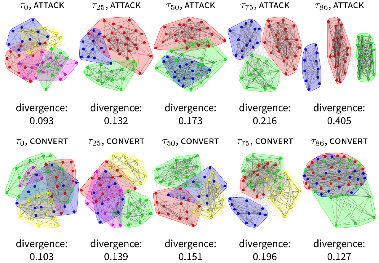
**Figure 4.** Development of clustering and group divergence for two sample debates through debate stages \(\tau_i\). The upper sample (attack strategy) shows tri-polarisation and monotonously increasing divergence values. The lower example (convert strategy) shows lower polarisation and signs of convergence.

Probably the most interesting feature of the attack series in Figure 4 is tri-polarisation in the last debate stage – especially when it is contrasted with convergence in the last debate stage of the convert series. There are two other differences. First, notice how the divergence is steadily increasing in the attack run, but developing non-monotonously in the convert run. This seems to show how the convert strategy is able to recover from increasing polarisation. Secondly, while both runs start with a high number of groups (5), the attack strategy very quickly reduces to only 3 groups, while the convert strategy is able to maintain its diversity until \(\tau_{25}\), and is able to uphold 4 groups until at least \(\tau_{75}\). This ability to maintain a higher diversity could be interpreted as contributing to the lower values observed in convert simulations.

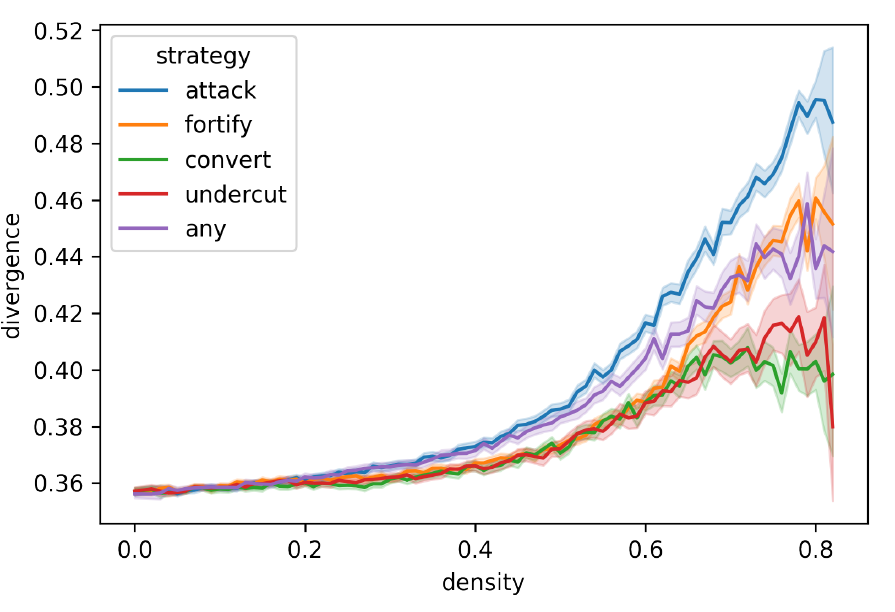
From the main experiment, the overall results for divergence depending on the two clustering algorithms are shown in Figure 5. As in the results for dispersion, these show how the introduction of arguments contributes to polarisation in general. More particularly, the attack strategy shows the highest polarisation values, while values particularly in undercut and convert seem to be more frequent in less polarised states. Values for the any strategy also lie between those of the four basic strategies, confirming the observation from the dispersion measurement. All together, this confirms the overall pattern from the dispersion values, although with considerably higher levels of polarisation.

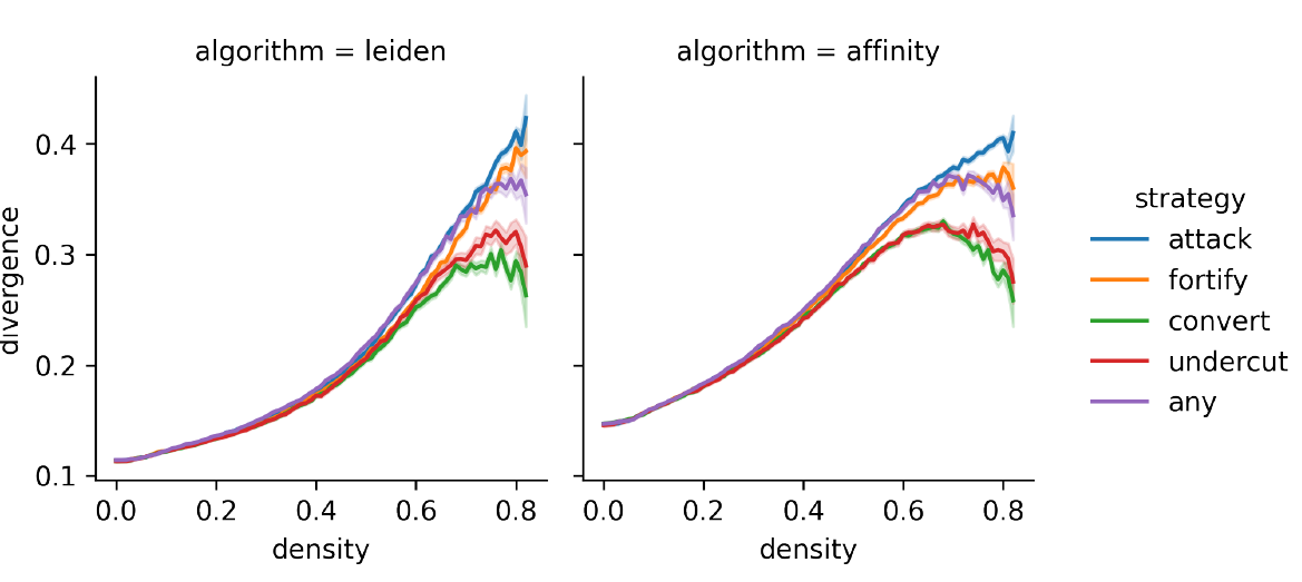
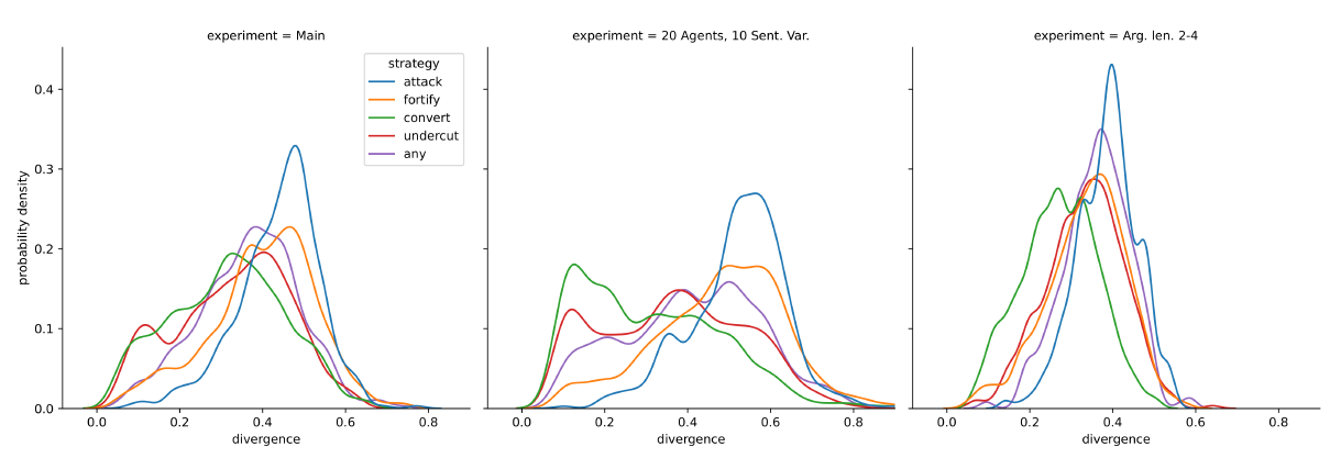
**Figure 5.** Mean divergence plotted against density, depending on argumentation strategies and clustering algorithms. Shaded areas indicate confidence intervals in terms of statistical bootstrapping.

Figure 6 takes a more concentrated look at the divergence data by showing the divergence distribution for the simulation runs as they reach a density of around 0.8. The panes compare the main experiment with two robustness analyses, and they show a noteworthy difference among argumentation strategies: convert and undercut model runs reach low levels of divergence much more often, and they have smoother distributions, whereas fortify and particularly attack model runs are single-peaked with a considerably lower chance of ending in low polarisation, an effect that remains stable in the robustness analyses (to be further discussed in the dedicated section below).

**Figure 6.** Distribution of divergence values based on Leiden clusterings at densities of around 0.8 for individual simulation runs in three different experiments. The area under each graph adds up to 100% of the divergence values, and the individual graphs show how the divergence values are distributed. For example, it shows that the convert strategy has a much higher proportion of model runs with a divergence of less than 0.2 at density 0.8 than the attack strategy, and that the biggest proportion of convert runs (about 20%) in the main experiment has a divergence of around 0.3, while the attack strategy peaks at around 0.5 with a proportion of more than 30%.

In quantitative terms (see Figure 14 in Appendix C), differences in group divergence are more pronounced than in dispersion, but the tendency is the same. In divergence analysed with the Leiden algorithm, 16% of simulation runs in the convert strategy have a group divergence of less than 0.2 – which is a very low increase, if any at all, from the start of the debate. For the attack strategy, only 0.8% of simulation runs reach this low level of polarisation. But about 43% of simulation runs with the attack strategy show moderate polarisation of at least 0.4, while only about 19% of convert debates do so. Fortify and undercut strategies are somewhere in between, with the fortify debates showing more tendency for medium polarisation and the undercut showing at least some chance of lower polarisation. The divergence mean for all data points at a density of around 0.8 is 0.29 for convert, but 0.41 for attack (see Table 2).

**Table 2:** Statistics on group divergence in simulation runs as they hit a density of 0.8, based on Leiden clusterings. (†) Note: Values for this robustness analysis is based on a sample of 400 simulation runs for each strategy, because not all 1,000 robustness runs reach densities of 0.8.
Sample	Total		Lowest 10%		Highest 10%
	Mean	SD	Mean	SD	Mean	SD
Main experiment
attack	0.41	0.09	0.24	0.05	0.54	0.04
fortify	0.39	0.11	0.17	0.05	0.55	0.03
convert	0.29	0.13	0.08	0.02	0.50	0.04
undercut	0.31	0.14	0.08	0.02	0.54	0.06
any	0.37	0.13	0.12	0.04	0.57	0.04
Agents: 20, Sentence variables: 10 (†)
attack	0.52	0.11	0.30	0.06	0.70	0.06
fortify	0.49	0.15	0.19	0.06	0.74	0.06
convert	0.30	0.17	0.10	0.00	0.62	0.06
undercut	0.38	0.18	0.11	0.01	0.68	0.05
any	0.40	0.17	0.12	0.02	0.68	0.08
Argument length: 2–4
attack	0.39	0.07	0.25	0.04	0.50	0.03
fortify	0.34	0.10	0.15	0.04	0.49	0.03
convert	0.27	0.10	0.10	0.02	0.43	0.03
undercut	0.33	0.09	0.16	0.04	0.48	0.03
any	0.36	0.08	0.20	0.04	0.49	0.04

Table 2 provides a possible explanation for the lower mean polarisation in convert and undercut: it might be due to their increased ability to reach states of very low polarisation more often (the lowest 10% of both strategies have a mean of 0.08, compared to 0.24 in attack). However, the strategies seem to differ less in their chance to reach higher values of polarisation, as the highest 10% of simulation runs have lower variation.

Qualifying the result that arguments drive polarisation on their own, two argumentation strategies, convert and undercut, have a higher chance to end in states of low polarisation, while the other two, fortify and attack, tend to drive moderate levels of polarisation. These tendencies are noteworthy because they run parallel to another distinction: fortify and attack are very much egocentric argumentation strategies insofar as they select premises from the source position. Convert and undercut are allocentric strategies by the same standard: the source devises an argument with premises that the target accepts. So it seems that, in agent-based debate models, egocentric premise selection can be a driver of moderate polarisation, which is most pronounced in the attack strategy, while allocentric premise selection has a higher chance of inducing states of lower polarisation, which is most pronounced in the convert strategy.

Group consensus

When a population of agents is clustered into groups, one can not only ask how much the groups differ, but also how high the agreement is in each individual group. Are they a tightly knit bunch or a more diverse group, in which disagreement may not be uncommon at all? Group consensus is aimed to measure this.

Definition 3. Group consensus, based on Bramson et al. (2016, pp. 91–92). Let \(\delta\) be the Hamming distance and \(G\) the clustering of the population at a debate stage with individual clusters \(g\). The expression \(\smash{g\choose 2}\) is understood to denote the set of agent pairs in \(g\). The debate’s consensus is then given as:

\[\text{consensus}(\tau) := 1- \frac{1}{|G|} \sum_{g=1}^{|G|} \frac{1}{\left|\left({g\atop 2}\right)\right|} \sum_{(x,y)\in \left({g\atop 2}\right)} \delta (x, y)\]

\[(7)\]

Group consensus measures how distant the members of groups are on average. This measure can capture situations in which the distance in groups is changing over time; contracting groups could be associated with lowering compatibility to outside influences, while rising distance between the group members could indicate that the groups are well acquainted to diversity of opinion and thus more open to outside influence. A rise in group divergence and a simultaneous rise in consensus captures an important part of the intuitive understanding of polarisation.

Figure 7 shows how group consensus develops amid the introduction of arguments in the main experiment. It is evident that group consensus correlates with density (Pearson’s \(r > 0.9, p \ll 0.001\) for all strategies), and that the variation between different strategies has a minor effect. Rising group consensus indicates that variance within groups diminish, but it does not automatically indicate that the groups move toward a more extreme stance than initially held by its members, and so this development does not quite confirm the law of group polarisation (Myers 1975; Sunstein 2002).

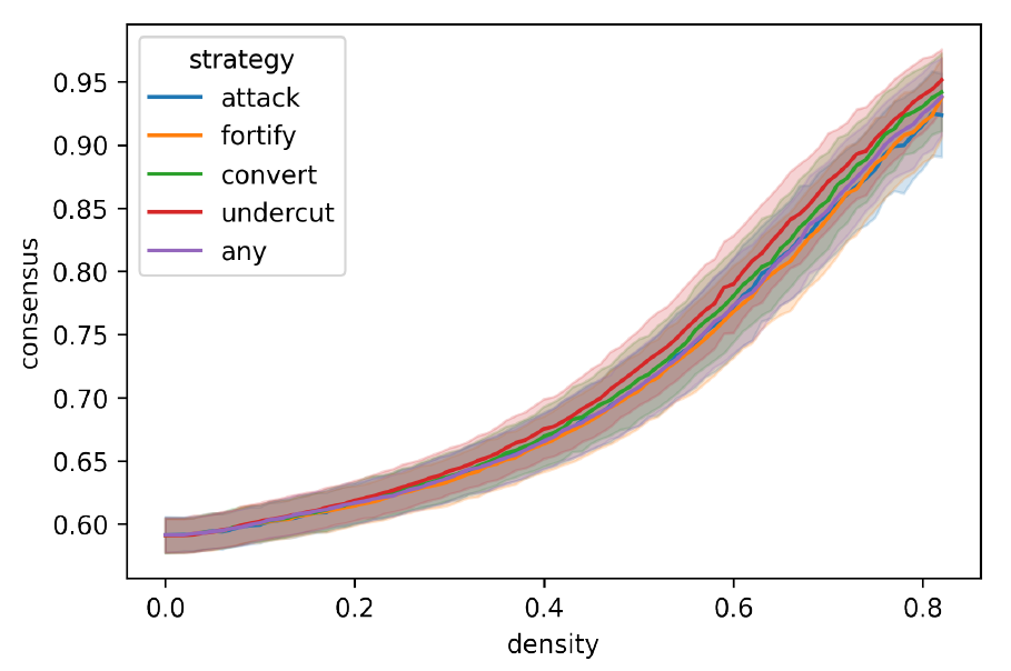
**Figure 7.** Development of group consensus in debates clustered with the Leiden algorithm, depending on argumentation strategy. Shaded areas show standard deviation.

It seems that the introduction of arguments, virtually irrespective of the employed argumentation strategy, can bring groups closer together. When evaluated together with the results from group divergence, there is a difference in which kind of group is, on average, produced by the argumentation strategies: while convert and undercut arguments lead to groups that are both in internal agreement and diverge less often from other groups, attack and fortify arguments have a more realistic chance to drive internally agreeing groups further apart, thus generating polarisation.

Robustness Analysis

Six experiments complement the main experiment, which has a population of 50 agents, 20 atomic sentence variables, and an argument length of 2–3 premises. The first four complementary experiments show that polarisation effects remain at least stable under variation of the initial settings concerning population size, extension of the sentence pool, and length of arguments. Table 2 from the previous section shows the mean values for group divergence at a density of 0.8 for the main experiment and two of these robustness analyses.

In a fifth robustness analysis, agents are not initialised with randomly assigned positions, but start off clustered into two groups with perfect bi-polarisation. This setting is designed to study the model’s behaviour concerning de-polarisation rather than polarisation. In the sixth and final analysis, the Leiden clustering is not obtained by taking into account agents’ complete positions, but only their stances on four propositions. This analysis is done to accommodate the fact that many real-world debates have a subset of sentences under discussion that are regarded to be the debate’s key issues.

20 agents debate 20 atomic sentence variables

The first variant, with 20 agents and the same sentence pool as in the main experiment, shows a slight amplification of the tendencies visible in the main experiment. For example, in group divergence based on Leiden, now 49% of model runs with the attack strategy end with divergences of at least 0.4 (+6%). Conversely, now 25% of runs with the convert strategy result in divergences below 0.2 (+9%). In the other argumentation strategies and in the dispersion measure, existing tendencies in the population of 50 are likewise slightly amplified in the population of 20. Group consensus remains stable.

20 agents debate 10 atomic sentence variables

But it is the second variation, with a population of 20 agents and 10 atomic sentence variables, that shows a considerable rise in polarisation. Figure 13 (Appendix C) shows the group divergence measure based on Leiden for densities of around 0.8 in this experiment, and the middle graph in Figure 6 visualises this distribution. Both plots show how the data now accumulates more toward the extremes. In the main experiment, almost a majority of attack and fortify model runs were in the \([0.3, 0.4)\) region. In the run with 10 agents, their largest groups are in the \([0.5, 0.6)\) region. The convert strategy shows a noteworthy shift toward the \([0.1, 0.2)\) region, and the undercut strategy a noteworthy distribution flattening: in the main experiment, its values spike in the \([0.3, 0.4)\) region, but now its data is more smoothly distributed throughout the \([0.1, 0.6)\) interval. In the other three strategies, one can observe the data to spread out in the direction already indicated in the main experiment. As a result, outcomes of high polarisation (\(\geq 0.8\)) have a non-zero probability, although still low at maximally 1.5% in the fortify strategy.

This seems to indicate that varying the population size or sentence pool in agent-based debate models with logical constraints does not have a uniform effect toward or against issue polarisation. The effect of these contracting or extending modifications is very much tied to the argumentation strategies, which I count as further evidence regarding their contribution toward polarisation in the model.

10 agents debate 5 atomic sentence variables with arguments of 2 premises

The effect can be even further amplified, as an experiment with 10 agents and five sentence variables shows. Here, the mean group divergence in attack is a staggering 0.67 at densities above 0.65, although the usefulness of this experiment is to be doubted considering that it is quite awkward to imagine a group of 10 agents to debate merely 5 atomic propositions for longer than just a few debate stages. These experiment settings lie on the lower bound of debates that can be feasibly simulated with the present model, as many debates do not reach a density of 0.8, and considering that agents produce arguments with two premises from a total of ten sentences, the argument introduction mechanism must be seen to work under heavy constraints with these settings. On the other end, the upper bound is not characterised by the agents’ abilities to devise arguments, but rather by limitations in computational complexity.

50 agents debate 20 atomic sentence variables with arguments of 2–4 premises

It may be more realistic to extend the number of premises that agents may use in devising arguments, up from a length of 2–3 premises that is allowed in the main experiment to 2–4 premises. This raises the initial size of the premise pool from 9,120 to 77,520.

The right graph in Figure 6 and Figure 14 (Appendix C) show the effect of this variation on group divergence at a density of 0.8. There is a contraction of data compared to the main experiment, with a minor amplification in attack and convert model runs: more model runs for attack end in the range for medium polarisation, and more convert runs end in low divergence (\(<0.3\)). The distributions in fortify and undercut are not amplified, but flattened. Overall, this study seems to confirm the results from the main experiment.

Initial bi-polarisation among 50 agents and 20 sentence variables

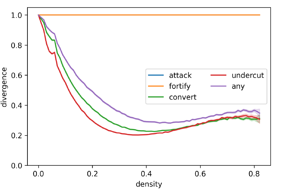
In all experiments discussed so far, agents start with randomly assigned positions. This means that the differences between agents is quite homogeneous on average, and so the observed polarisation values are always relatively low at the beginning of a model run. This raises the question how the model behaves when the population starts highly polarised. In this robustness analysis, perfect bi-polarisation is induced by splitting the population of 50 agents in half, and assigning the same position to each agent in each half. All agents in the first group start by assigning True to the first half of sentences, but False to the other half (\(\{ \{p_0,p_1,...,p_9\} \to \text{True}, \{p_{10},p_{11},...,p_{19}\} \to \text{False} \}\)), and the agents in the second group hold the exact inverse at the start (\(\{ \{p_0,p_1,...,p_9\} \to \text{False}, \{p_{10},p_{11},...,p_{19}\} \to \text{True} \}\)). This creates an initial perfect bi-polarisation in terms of group divergence (see Figure 8).

There is a striking difference between the argumentation strategies as they respond to initially bi-polarised debates. While the strategies that select premises allocentrically (convert and undercut) show significant effects of de-polarisation, the egocentric strategies (attack and fortify) prove unable to recover from a state of bi-polarisation. Populations that use only these strategies remain at a state of bi-polarisation throughout the debate, while the convert and undercut strategies quickly lead to significantly lower polarisation levels. When allocentrism and egocentrism in premise choice are mixed in the any strategy, the outcome is mixed as well: de-polarisation occurs, but at a lower rate than in the purely allocentric strategies.

**Figure 8.** Group divergence following Leiden clusterings for an experiment with 50 agents and 20 atomic sentence variables in which the agents start in perfect bi-polarisation. The graphs for the attack and fortify strategies are exactly the same and overlap in this plot.

Clustering on a subset of propositions

The clusterings in the evaluation above take into account agents’ complete positions, which assumes that all sentences under discussion are equally relevant in determining the groups. Yet debates often evolve around a set of key issues. For these, it may be more realistic to cluster agents into groups depending only on their stance toward these key issues. Figure 9 shows the results of such a clustering on a subset of the sentence pool consisting in four propositions. The debate stages from the main experiment are used for this analysis, but instead of using agent’s complete positions for the clustering, it asks how the population would have been clustered if only these four propositions had been taken into account. The results confirm the main findings, but there is significantly more volatility in the data.

**Figure 9.** Group divergence following a Leiden clustering on the main experiment, but on a subset of four key propositions from the sentence pool.

Conclusion

Summary of results

In this paper, I studied an agent-based debate model based on the theory of dialectical structures. It models a population in which agents update their perspective due to logical constraints, but not based on social factors such as similarity or trust. A simulation experiment of 5000 model runs revealed that arguments can generally be a driver of issue polarisation, and that argumentation strategies affect it differently. This result was confirmed in a robustness analysis. In dispersion and group divergence, two state-of-the-art measures for issue polarisation, argumentation strategies that behave egocentrically (attack and fortify) in the selection of premises were associated with significantly higher levels of polarisation compared to strategies that select premises allocentrically (convert and undercut). All argumentation strategies increased issue polarisation similarly when observed in a third measure, group consensus. Besides the general influence of arguments on polarisation, the picture that emerged here was that the attack and fortify strategies simultaneously lead to groups being more alike internally and more distant compared to other groups, while convert and undercut produced groups that, albeit rising internal consensus, did not move apart from other groups that much.

The argumentation strategies also significantly differed in their ability to recover from bi-polarisation: when agents used the allocentric strategies or a mixed strategy (“any”), they were able to de-polarise debates with initial bi-polarisation. However, the egocentric strategies failed to recover from perfect bi-polarisation and did not show any ability to de-polarise.

The model shows that polarisation is possible among artificial agents by means of rational processes. Introducing arguments and responding to those of others in a rational manner influences the polarisation dynamics in this model by showing how a initially unpolarised population can move to medium levels of polarisation, and how populations that differ in their argumentation strategy also differ in their ability to de-polarise an initial setting of perfect bi-polarisation. The argumentative, rational behaviour is the sole driver inspected in this model, but it is for future research to inspect polarisation dynamics as argumentation interacts with other factors.

Limitations

The model presented here is intended to understand issue polarisation in a specific kind of artificial agent. The agents are modelled to have bounded rationality and always follow the same argumentation and updating strategies, without making any errors in applying them. The results from simulations on this model should not be directly applied in interpretation of human behaviour and/or states of social polarisation. Rather, this model elucidates properties of argumentative features irrespective of other variables, of which there are quite a few.

On a minor note, Polberg & Hunter (2018) stress the importance of modelling (a) bipolar argumentation, allowing for both support and defeat relations in agent-based debate models, but also of modelling (b) probabilistic belief systems. The model presented here fulfils their requirement (a) but falls short of fulfilling (b), mainly due to computational restrictions. An extension of the model to probabilistic belief systems is left for future research.

As mentioned above, the simulation results fall short of producing high and very high polarisation values. This is in contrast to some social influence models (Banisch & Olbrich 2021; Mäs & Flache 2013), which often end in states of perfect bi-polarisation. Yet this inability to produce perfect bi-polarisation should be seen as a virtue rather than a vice. If argumentation alone were to explain high and very high degrees of issue polarisation among artificial agents, there would be no room to accommodate other factors in extended models. The factors not considered in this model include homophily, limited agent memory, and bias in selection of communication partners relative to argumentation strategy. Extensions of this model could consider if there should not be some bias in selecting a target position given some of the argumentation strategies: for example, what changes if agents only attack out-group targets?

Acknowledgements

I’m indebted to Gregor Betz for extensive and insightful discussions. I thank my colleagues at KIT for discussing a draft of this paper, particularly Christian Seidel and Michael Poznic. I would also like to express my gratitude to three anonymous reviewers for their helpful comments and suggestions. Among other things, I added an analysis of the any strategy as well as the initially polarised robustness analysis following their comments. I also gratefully acknowledge support by the state of Baden-Württemberg through bwHPC, the state’s high performance computing consortium. Last but not least, I gratefully acknowledge support by the KIT Publication Fund of the Karlsruhe Institute of Technology for covering publication costs.

Appendix

Appendix A: Data and code sources

A repository at https://doi.org/10.5281/zenodo.5067834 is released together with this paper. It contains:

The complete simulation runs including data on positions and arguments as pickled Python objects. These can be loaded with pickle.load().
Raw measurement values for each polarisation measure, as well as the raw ARI values, as zipped DataFrames. These data can be directly loaded in Python with pandas.read_pickle().
A Jupyter notebook from which the simulation experiments can be run.
Jupyter notebooks which show the data analysis done for this paper. These notebooks also contains all the code to generate the figures shown in this paper.
Source code and documentation of taupy in the version used in this paper. taupy, a Python package to study the theory of dialectical structures, serves as backbone for the model presented in this paper.

Appendix B: Complementary measurements and data

**Figure 10.** Distribution of ARI values for all pairs (\(N=543,958\)) of adjacent debate stages depending on argumentation strategy in Leiden clusterings. Boxes represent 50% of the respective data and show the median. Box and whiskers represent 95% of the data, while outliers mark 5% of the data.

**Figure 11.** Average number of agents which update their positions at time \(\tau_i\) following argument introduction in debate stage \(\tau_{i-1}\) depending on argumentation strategy and plotted against the averaged density of the two stages \(\tau_i, \tau_{i-1}\).

**Figure 12.** Development of density over simulation time (in terms of debate stages) depending on argumentation strategy and averaged over all model runs in the main experiment. Here, attack and fortify model runs can take considerably more simulation time to reach the termination density of 0.8.

Appendix C: Raw polarisation values

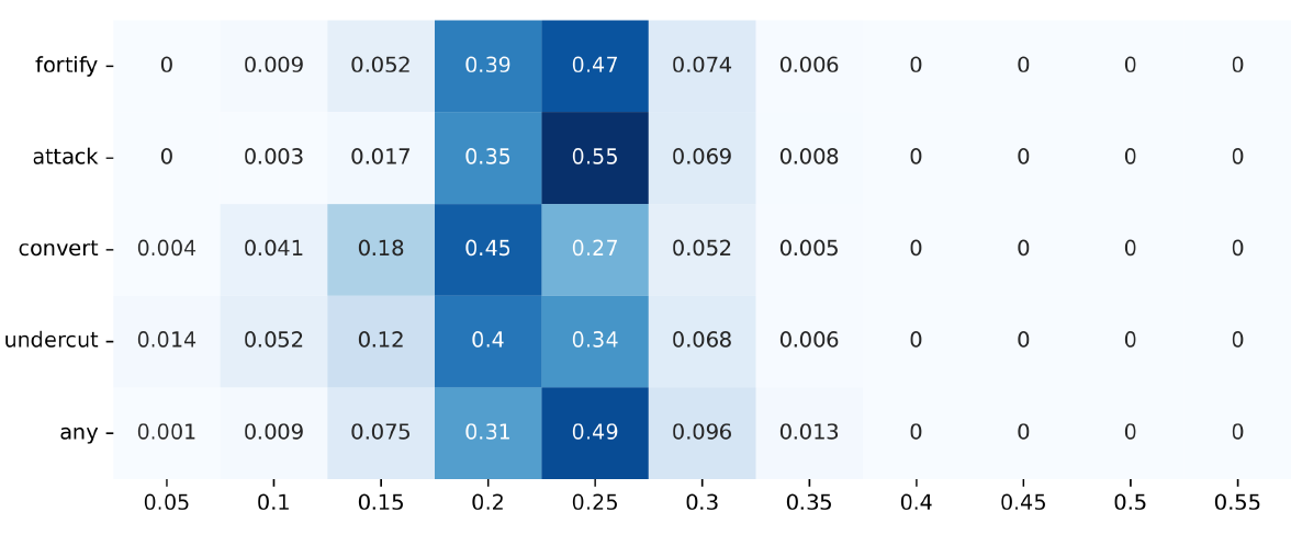
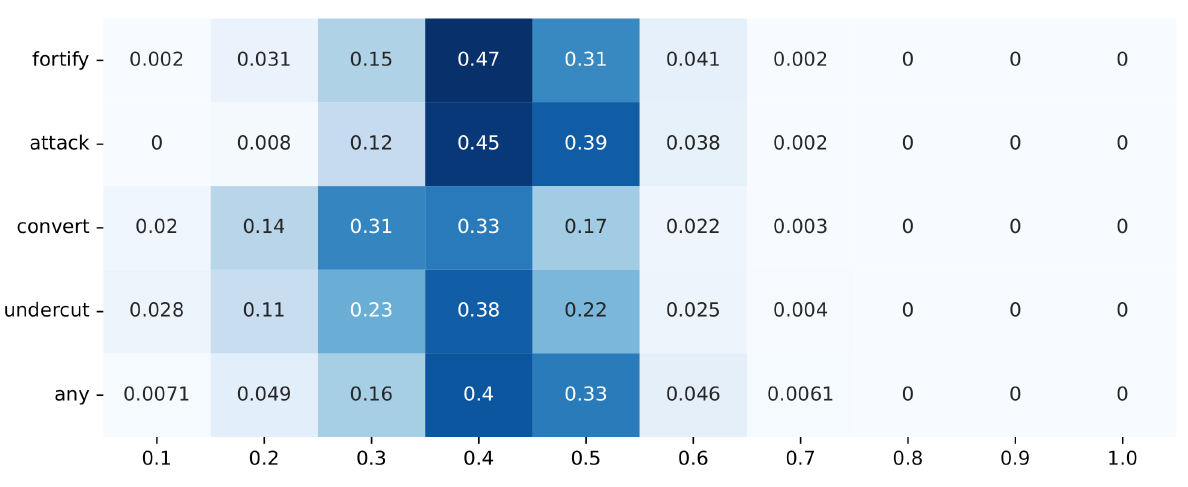
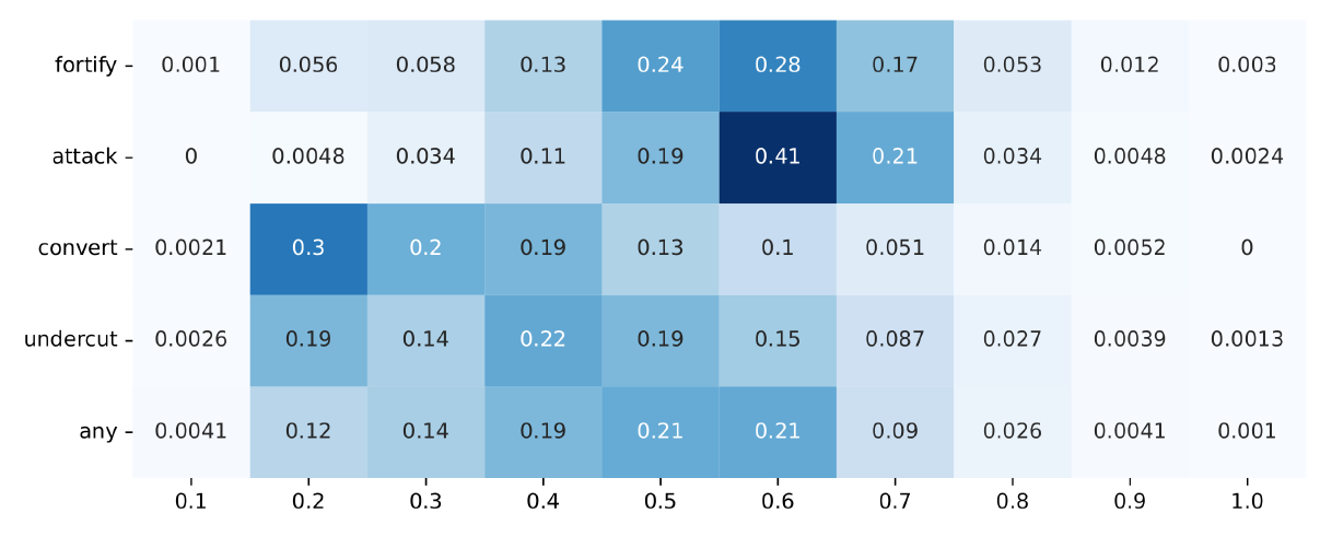
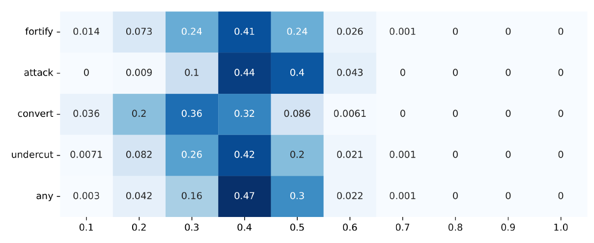
The plots in this appendix display raw polarisation values. They are interpreted as heat maps in tabular alignment, where the x-axis shows polarisation intervals and the cells contain the proportion of model runs in the respective argumentation strategy that lie in this interval as they reach a density of at least 0.8.

**Figure 13.** Histogram of dispersion values at the first debate stage of each simulation run that passes a density of 0.8, interpreted as a heat map. For every \(i\) on the x axis, the area assigned to it shows values in the half-open interval \([i-1,i)\). For example, the tick 0.25 shows the proportion of observed values in the interval \([0.2, 0.25)\) relative to all observed values of the same strategy. Since there are 1,000 simulation runs in each strategy, absolute values can be easily obtained from the relative values.

**Figure 14.** Distribution of simulation runs and their group divergence values based on clusterings from the Leiden algorithm at densities of around 0.8. For every \(i\) on the x axis, the area assigned to it shows values in the half-open interval \([i-1,i)\). (Data for main experiment with 50 agents and 20 atomic sentence variables).

**Figure 15.** Polarisation distribution measured as group divergence based on a clustering from the Leiden algorithm for simulation runs as they reach a density of 0.8 (data for control experiment with 20 agents and 10 atomic sentence variables).

**Figure 16.** Distribution of simulation runs and their group divergence based on clusterings from Leiden at densities of around 0.8. Data for control experiment with argument length of 2–4.

References

BANISCH, S., & Olbrich, E. (2021). An argument communication model of polarization and ideological alignment. Journal of Artificial Societies and Social Simulation, 24(1), 1: https://www.jasss.org/24/1/1.html. [doi:10.18564/jasss.4434]

BESNARD, P., & Hunter, A. (2008). Elements of Argumentation. Cambridge, MA: MIT Press.

BETZ, G. (2009). Evaluating dialectical structures. Journal of Philosophical Logic, 38, 283–312. [doi:10.1007/s10992-008-9091-5]

BETZ, G. (2013). Debate Synamics: How Controversy Improves Our Beliefs. Berlin Heidelberg: Springer.

BETZ, G. (2021). Natural-language multi-agent simulations of argumentative opinion dynamics. Journal of Artificial Societies and Social Simulation, 25(1), 2: https://www.jasss.org/25/1/2.html. [doi:10.18564/jasss.4725]

BRAMSON, A., Grim, P., Singer, D. J., Berger, W. J., Sack, G., Fisher, S., & Flocken, C. (2016). Disambiguation of social polarization concepts and measures. The Journal of Mathematical Sociology, 40(2), 80–111. [doi:10.1080/0022250x.2016.1147443]

BUTLER, G., Pigozzi, G., & Rouchier, J. (2019). Mixing dyadic and deliberative opinion dynamics in an agent-based model of group decision-making. Complexity, 2019, 3758159. [doi:10.1155/2019/3758159]

CAYROL, C., & Lagasquie-Schiex, M. C. (2005). 'On the acceptability of arguments in bipolar argumentation frameworks.' In L. Godo (Ed.), Symbolic and Quantitative Approaches to Reasoning With Uncertainty, ECSQARU 2005 (Lecture Notes in Computer Science, Vol. 3571). Berlin Heidelberg: Springer. [doi:10.1007/11518655_33]

CSÁRDI, G., & Nepusz, T. (2006). The igraph software package for complex network research. InterJournal Complex Systems, 1695.

DUNG, P. M. (1995). On the acceptability of arguments and its fundamental role in nonmonotonic reasoning, logic programming and n-person games. Artificial Intelligence, 77(2), 321–357. [doi:10.1016/0004-3702(94)00041-x]

FLACHE, A., Mäs, M., Feliciani, T., Chattoe-Brown, E., Deffuant, G., Huet, S., & Lorenz, J. (2017). Models of social influence: Towards the next frontiers. Journal of Artificial Societies and Social Simulation, 20(4), 2: https://www.jasss.org/24/4/2.html. [doi:10.18564/jasss.3521]

FREY, B. J., & Dueck, D. (2007). Clustering by passing messages between data points. Science, 315(5814), 972–976. [doi:10.1126/science.1136800]

FRIEDKIN, N. E., Proskurnikov, A. V., Tempo, R., & Parsegov, S. E. (2016). Network science on belief system dynamics under logic constraints. Science, 354(6310), 321–326. [doi:10.1126/science.aag2624]

GRIMM, V., Berger, U., Bastiansen, F., Eliassen, S., Ginot, V., Giske, J., Goss-Custard, J., Grand, T., Heinz, S. K., Huse, G., Huth, A., Jepsen, J. U., Jørgensen, C., Mooij, W. M., Müller, B., Pe’er, G., Piou, C., Railsback, S. F., Robbins, A. M., Robbins, M. M., Rossmanith, E., Rüger, N., Strand, E., Souissi, S., Stillman, R. A., Vabø, R., Visser, U. & DeAngelis, D. L. (2006). A standard protocol for describing individual-based and agent-based models. Ecological Modelling, 198(1-2), 115–126. [doi:10.1016/j.ecolmodel.2006.04.023]

HUBERT, L., & Arabie, P. (1985). Comparing partitions. Journal of Classification, 2, 193–218.

HUNTER, A., Chalaguine, L., Czernuszenko, T., Hadoux, E., & Polberg, S. (2019). 'Towards computational persuasion via natural language argumentation dialogues.' In C. Benzmüller & H. Stuckenschmidt (Eds.), KI 2019: Advances in Artificial Intelligence (pp. 18–33). Lecture Notes in Computer Science, Berlin Heidelberg: Springer. [doi:10.1007/978-3-030-30179-8_2]

IYENGAR, S., Lelkes, Y., Levendusky, M., Malhotra, N., & Westwood, S. J. (2019). The origins and consequences of affective polarization in the United States. Annual Review of Political Science, 22, 129–146. [doi:10.1146/annurev-polisci-051117-073034]

IYENGAR, S., Sood, G., & Lelkes, Y. (2012). Affect, not ideology: A social identity perspective on polarization. Public Opinion Quarterly, 76(3), 405–431. [doi:10.1093/poq/nfs059]

KEIJZER, M. A., Mäs, M., & Flache, A. (2018). Communication in online social networks fosters cultural isolation. Complexity, 2018, 9502872. [doi:10.1155/2018/9502872]

MASON, L. (2013). The rise of uncivil agreement: Issue versus behavioral polarization in the American electorate. American Behavioral Scientist, 57(1), 140–159. [doi:10.1177/0002764212463363]

MASON, L. (2015). “I disrespectfully agree”: The differential effects of partisan sorting on social and issue polarization. American Journal of Political Science, 59(1), 128–145. [doi:10.1111/ajps.12089]

MÄS, M., & Flache, A. (2013). Differentiation without distancing: Explaining bi-polarization of opinions without negative influence. PLoS ONE, 8(11), e74516. [doi:10.1371/journal.pone.0074516]

MCPHERSON, M., Smith-Lovin, L., & Cook, J. M. (2001). Birds of a feather: Homophily in social networks. Annual Review of Sociology, 27(1), 415–444. [doi:10.1146/annurev.soc.27.1.415]

MERDES, C., von Sydow, M., & Hahn, U. (2020). Formal models of source reliability. Synthese, 198(2021), 5773–5801. [doi:10.1007/s11229-020-02595-2]

MUTZ, D. C. (2002). Cross-cutting social networks: Testing democratic theory in practice. American Political Science Review, 96(1), 111–126. [doi:10.1017/s0003055402004264]

MYERS, D. G. (1975). Discussion-induced attitude polarization. Human Relations, 28(8), 699–714. [doi:10.1177/001872677502800802]

OLSSON, E. J. (2013). 'A Bayesian simulation model of group deliberation and polarization.' In F. Zenker (Ed.), Bayesian Argumentation: The Practical Side of Probability. Dordrecht: Springer. [doi:10.1007/978-94-007-5357-0_6]

PALLAVICINI, J., Hallsson, B., & Kappel, K. (2021). Polarization in groups of Bayesian agents. Synthese, 198, 1–55. [doi:10.1007/s11229-018-01978-w]

PEDREGOSA, F., Varoquaux, G., Gramfort, A., Michel, V., Thirion, B., Grisel, O., Blondel, M., Prettenhofer, P., Weiss, R., Dubourg, V., Vanderplas, J., Passos, A., Cournapeau, D., Brucher, M., Perrot, M., & Duchesnay, E. (2011). Scikit-learn: Machine learning in Python. Journal of Machine Learning Research, 12, 2825–2830.

PEW Research Center. (2014). Political polarization in the American public: How increasing ideological uniformity and partisan antipathy affect politics, compromise and everyday life. Available at: https://www.people-press.org/2014/06/12/political-polarization-in-the-american-public/.

POLBERG, S., & Hunter, A. (2018). Empirical evaluation of abstract argumentation: Supporting the need for bipolar and probabilistic approaches. International Journal of Approximate Reasoning, 93, 487–543. [doi:10.1016/j.ijar.2017.11.009]

SUNSTEIN, C. R. (2002). The law of group polarization. The Journal of Political Philosophy, 10(2), 175–195.

TRAAG, V. A., Waltman, L., & van Eck, L. J. (2019). From Louvain to Leiden: Guaranteeing well-connected communities. Scientific Reports, 9(2019), 5233. [doi:10.1038/s41598-019-41695-z]